Magnetic Stereoscopy
Abstract
The space mission STEREO will provide images from two viewpoints. An important aim of the STEREO mission is to get a 3D view of the solar corona. We develop a program for the stereoscopic reconstruction of 3D coronal loops from images taken with the two STEREO spacecraft. A pure geometric triangulation of coronal features leads to ambiguities because the dilute plasma emissions complicates the association of features in image 1 with features in image 2. As a consequence of these problems the stereoscopic reconstruction is not unique and multiple solutions occur. We demonstrate how these ambiguities can be resolved with the help of different coronal magnetic field models (potential, linear and non-linear force-free fields). The idea is that, due to the high conductivity in the coronal plasma, the emitting plasma outlines the magnetic field lines. Consequently the 3D coronal magnetic field provides a proxy for the stereoscopy which allows to eliminate inconsistent configurations. The combination of stereoscopy and magnetic modelling is more powerful than one of these tools alone. We test our method with the help of a model active region and plan to apply it to the solar case as soon as STEREO data become available.
keywords:
STEREO, magnetic fields, extrapolations1 Introduction
The forthcoming space mission STEREO (Solar TErrestrial RElations Observatory) will observe the Sun simultaneously from two viewpoints. One aim of the mission is to reconstruct the solar corona in three dimensions (see, e.g., \openciteschmidt:etal96; \opencitegary:etal98 for an overview). To do so we have to develop tools for the stereoscopic reconstruction of the 3D corona from two STEREO-images. A triangulation method using the solar rotation has been applied to Skylab images by \inlineciteberton:etal85 and \inlinecitebatchelor94. Aschwanden et al.(1999, 2000) and \inlineciteportier-fozzani:etal01 used SOHO data and the rotation of the Sun for a stereoscopic reconstruction. Using the rotation of the Sun and taking images a few days apart allows of course only the reconstruction of features with remain stationary within this time. \inlineciteaschwanden:etal99 made a fit of the observed loop structures to sections of circles and allowed for a time dependence of some of the fit parameters. The method was called dynamic stereoscopy and used the assumption of circular coronal loops as a priori information. \inlinecitewiegelmann:etal02 demonstrated how the 3D loops published in Aschwanden et al. (1999) and photospheric magnetic field measurements can be used to compute a corresponding coronal magnetic field model within the linear force-free model. A basic assumption was that due to the high conductivity the emitting coronal plasma also outlines the magnetic field. The alignment of coronal plasma and magnetic field lines has also be used directly with 2D images from (Yokoh/SXT) in Carcedo et al. (2003) and from (SOHO/EIT) in Marsch, Wiegelmann and Xia (2004) to compute the optimal coronal magnetic field within the linear force-free assumption. \inlinecitewiegelmann:etal05b used linear and non-linear force-free magnetic field models for the identification of coronal loops in EUV images.
The aim of this work is to develop a tool for the stereoscopic reconstruction of coronal features (mainly closed loops in active regions) from two viewpoints. We test the quality of our reconstruction tools with the help of a model active region. Pure geometric stereoscopy leads to multiple solutions, mainly because the faint coronal plasma does not allow a clear association of features in both Stereo-images with each other. Classical stereoscopy works best for objects with clear edges in images with high contrast. Unfortunately this is not the case in the solar corona where the plasma structures are very faint and diffuse, e.g., visible loops in high-resolution TRACE images are often a superposition of several individual loops (Schrijver et al., 1999, 2004).
We demonstrate how a suitable coronal magnetic field model can be used to find the association of loops in the STEREO images and thereby remove ambiguities in the stereoscopic reconstruction. The method also tell us, how well the assumed coronal magnetic field model aligns observed loops in both images and computes (for linear force-free models) the optimal value of . The tools are planned for use within the STEREO-mission.
2 Stereoscopy tools
2.1 Geometric Stereoscopy
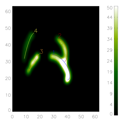
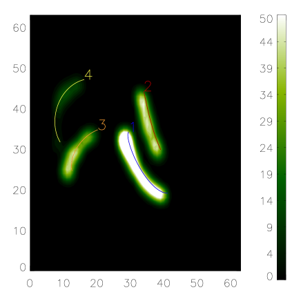
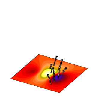
By geometric stereoscopy we understand a 3D reconstruction from two images, e.g., from the projections as shown in Figure 3. As real STEREO data are not yet available, we test our method with the help of a model active region, as described in appendix A. Using a model active region helps us (because we know the true solution) to check how accurate our stereoscopic reconstruction tools work. Here we try to reconstruct the four loops in 3D from the artificial images shown in Figure 3. For real observed images from e.g., the two STEREO-spacecraft one needs to get the loops (or after \openciteaschwanden05 curvi-linear 1D features.) first from the 2D EUV images by feature tracking method. Several methods have been proposed for this aim, e.g., the brightness-gradient method and the oriented-connectivity method (See \openciteaschwanden05; \opencitelee:etal06 for an overview). Here we concentrate on the 3D reconstruction and assume that the two EUV images have been transformed into curvi-linear 1D features. In the following we call these observed elongated structures in EUV-images simply loops. In contrast field lines are 3D curves derived from magnetic field models. The assumption is that loops and projections of field lines are aligned.
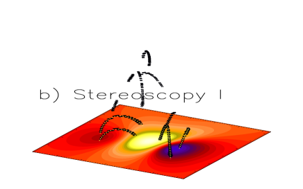
We make a back projection of the 4 images into the original 3D box. Geometric stereoscopy works well for solid objects with well distinguishable edges. If one has correctly identified two related points in both images, a computation of the 3D location of the point is straight forward. One just has to calculate the point of intersection along the line-of-sight of both images. Unfortunately the situation is more complicated for the solar corona. Coronal loops are faint elongated objects and often have no clearly visible edges. It is not clear a priori which points along a loop projection in image 1 belong to which points along the same loop from another viewpoint in image 2. The situation becomes even worse for multiple loops which are close together in the images. Here it is not always possible to distinguish which loops from image 1 correspond to which loops in image 2. For a stereoscopic reconstruction in such a situation we compute the intersection points of all identified loop points in image 1 with all identified loop points in the second image 111It is sufficient to search for intersection points which are on the same epipolar line, because points on different epipolar lines do not intersect.. The 3D reconstruction is not unique, however, because a pixel in one image usually intersects with more than one pixel in the other image. An example of a pure geometric stereoscopic reconstruction is shown in Figure 2 b). The black pixels mark the 3D intersection of the 3D reconstruction, the yellow dotted lines mark the original loops. One can see that geometric stereoscopy finds the correct 3D locations of the loops and reconstructs the original loop structure, but also several ghost features occur, which are not related to any real loop. The challenge is to identify which intersections are real and correspond to magnetic loops on the Sun and to eliminate the ghost points.
2.2 Magnetic modelling
While the blurring and the line-of-sight character of the coronal images complicate the interpretation, the coronal plasma has the nice feature that the plasma emission outlines the magnetic field. This is a consequence of the high conductivity of the coronal plasma. Outlining means that the loops visible in EUV images also represent projections of the magnetic field lines. Consequently the 3D reconstruction of coronal plasma loops and 3D magnetic field lines are associated with each other. Unfortunately the 3D coronal magnetic field cannot be measured directly and one has to extrapolate the field from photospheric measurements into the corona. The extrapolation depends on assumptions regarding the coronal plasma, in particular the electric current density. In the low and middle corona the magnetic pressure dominates over the plasma pressure ( ) which allows to use force-free magnetic field models. Force-free magnetic fields have to obey the equations
| (1) | |||||
| (2) |
which are equivalent to
| (3) | |||||
| (4) |
The in general non-linear force-free field model Sakurai (1981); Amari, Boulmezaoud and Mikic (1999); Wheatland, Sturrock and Roumeliotis (2000); Yan and Sakurai (2000); Régnier, Amari and Kersalé (2002); Wiegelmann and Neukirch (2003); Wiegelmann (2004); Wheatland (2004); Valori, Kliem and Keppens (2005); Wiegelmann, Inhester and Sakurai (2006); Inhester and Wiegelmann (2006) has potential fields (no currents, e.g., \opencitesemel67) and linear force-free fields (current proportional to the magnetic field with a global constant , e.g., \opencitechiu:etal77;\openciteseehafer78) as subclasses. Potential and linear force-free fields only need the line-of-sight magnetic field as input, which is observed routinely from e.g., SOHO/MDI and NSO/Kitt Peak. Non-linear force-free fields are mathematically more challenging to compute and require photospheric vector magnetograms as input. Such data contain high noise and ambiguities in the transverse magnetic field component and currently operating vectormagnetographs (e.g., NAO/SFT, VTT in Tenerife and IVM in Hawaii) have a limited field of view. The observational shortage of vectormagnetograph data will improve however in the near future with the forthcoming missions Solar-B, SOLIS and SDO. The non-linear force-free approach describes the magnetic field in active regions more accurately than potential and linear force-free fields (see \opencitewiegelmann:etal05).
2.2.1 Potential and linear force-free fields.
We use the Seehafer (1978) method to calculate potential and linear force-free fields. The method requires a photospheric line-of-sight magnetogram (e.g., from SOHO/MDI) as input. The Seehafer solution is computed on a rectangular grid and and contains the free force-free parameter , which cannot be evaluated from the observed line-of-sight magnetic field. To normalize we choose the harmonic mean of and defined by . The force-free parameter is limited by Potential fields correspond to . (See \openciteseehafer78 for details.)
2.2.2 Non-linear force-free fields.
We solve Eqs. (1) and (2) with the help of an optimization principle as proposed by \inlinecitewheatland:etal00 and generalized by \inlinecitewiegelmann:etal03a; \inlinecitewiegelmann04:
| (5) |
where is a weighting function. It is obvious that (for ) the force-free Eqs. (1-2) are fulfilled when L equals zero. As an initial configuration we compute a potential magnetic field in the computational box. As the next step we use photospheric vector magnetic field data to prescribe the bottom boundary (photosphere) of the computational box. On the lateral and top boundaries the field is chosen from the potential field above. We iterate for the magnetic field inside the computational box by minimizing Eq. (5). The weighting function equals 1 everywhere in the computational box except in a boundary layer of points towards the lateral and top boundary of the computational box, where decreases smoothly to 0 with a cosine function. (See \opencitewiegelmann04 for details of our implementation of the non-linear force-free optimization principle.)



3 How does the magnetic field help us with stereoscopy?
The scheme in Figure 1 outlines how information regarding the coronal magnetic field can be used to improve the stereoscopic reconstruction. A key question is to associate coronal features, e.g., loops in image 1 (from the STEREO-1 spacecraft) with features in image 2 (observed from STEREO-2). In the following we specify some details of the scheme.
-
1.
A first step is to segment the 2D images into loops. This is by no means a trivial process and several methods have been proposed, e.g., the brightness gradient method, the oriented-connectivity method, magnetic field extrapolation and curvature radius constraints and the use of multiple temperature filters. An overview about current developments for this step is given in Aschwanden (2005); Lee, Newman and Gary (2006).
-
2.
The next step requires a suitable magnetic field model. As the coronal magnetic field can usually not be measured directly, we extrapolate it from photospheric magnetic field measurements (from vector or line-of-sight magnetographs). The coronal magnetic field model may also contain additional parameters, e.g., the linear force-free parameter . An overview about coronal magnetic field models is given in section 2.2. We use a fourth order magnetic field line tracer to compute 3D magnetic field lines from the 3D magnetic field. The starting points are chosen randomly, magnetic flux weighted, on the photosphere and in the current implementation only closed magnetic loops (both footpoints are on the photosphere) are stored because the main application is to identify closed coronal loops, see also Wiegelmann et al. (2005a). Open field lines are expected not to be visible anyway. As a result we get space filling magnetic field lines in 3D. A basic assumption is that the emitting plasma loops also outline the coronal magnetic field. This is a consequence of the high conductivity of the coronal plasma. The emissivity gradient along the magnetic field is much smaller than in the perpendicular direction.
-
3.
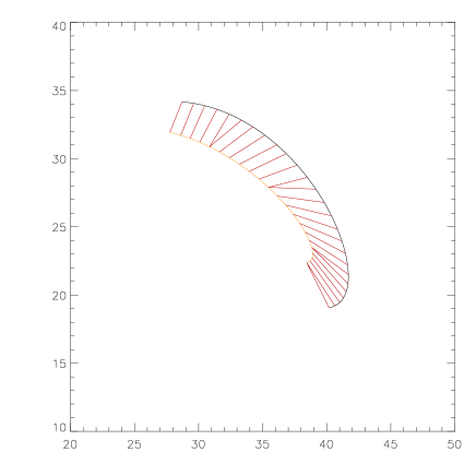
The 3D magnetic field lines are projected onto both images from the two STEREO-spacecraft. For every projected field line we measure how well it agrees with one of the loops identified in step one. As a measure of this agreement we take the area between each loop and the projections of the magnetic field line in each image (see lower right panel in Figure 4) normalized by the length of the respective loop. The measure then corresponds to the average distance of the loop and the projection of the 3D magnetic field line. Perfect agreement corresponds to . If is the number of field lines and the number of loops in image ( or ) we get a matrix of the dimension for image one and another matrix for image two, which contain the corresponding values and . We here give C in units of a pixel size to have a clear relation to the image resolution.
-
4.
The next step is to associate the loops in both images which each other. The aim is to find for each pair of loops and a magnetic field line for which the summed measures and are minimal. As a result of this step we get a matrix which contains the arithmetic mean of from both images for all possible association between image 1 and image 2. can be calculated for each magnetic field line. The optimal magnetic field line corresponds to the minimum of in . Again, corresponds to perfect agreement. Figure 4 contains a stacked histogram-style plot for this matrix ( matrix for the four loops features shown in Figure 3 from two viewpoints. We preferred to plot instead of for a better visualization. Here high values of correspond to a good agreement, e.g., a value of means that the projection of the field line and the loop are in average only one fifth of a pixel apart.) The absolute values certainly depend on the chosen magnetic field model and partly also on the number of field lines plotted in step 2.
For a good magnetic field model one has a clear association of features in image 1 with features in image 2 after this step already. This is certainly the case for the non-linear force-free model shown in the lower left panel of Figure 4. The method correctly associates loop 1 of image 1 with loop 1 of image 2 etc. with values of . , which gives an average measure of .
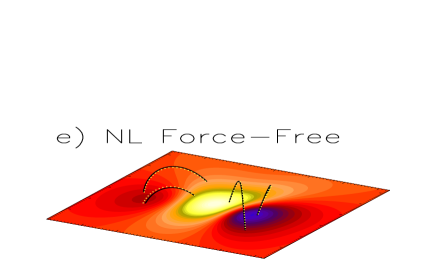
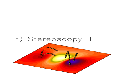
As a consequence the 3D magnetic field lines are already an excellent proxy for the 3D loop and an explicit geometric stereoscopic reconstruction is not necessary anymore. Figure 2 e) shows the four identified magnetic field lines in black and the original model loops dotted in yellow. The picture shows an agreement of original and reconstruction within plotting precision.
The loop association with help of potential and linear force-free fields (upper left and right panel in Figure 4) is not as good as for the non-linear force-free case. The linear force-free model associates the loops in both images with a distance of or in average . All loops are associated correctly. The linear force-free model provides us also the optimal values of for each loop, which are for loop 1 and 2 and for loop 3 and 4. Different values of on different loops are a contradiction to the assumption of a linear force-free model, which requires a single global value of . So the loop association method tells us also whether a linear force-free field is a fair approximation for the coronal magnetic field ( is identical or almost identical for all loops) or not. In this example it is not. Nevertheless the optimal linear-force free 3D magnetic field lines are a proxy for the 3D plasma loop. The proxy is the better the smaller the correspondent values of . Figure 2 d) shows the four proxy field lines for the linear force-free case. In accordance with the values of the matrix (upper right panel of Figure 4) we get a very good agreement with the original for loop 3, some small deviations for loop 4 and larger deviations for loop 1 and 2.
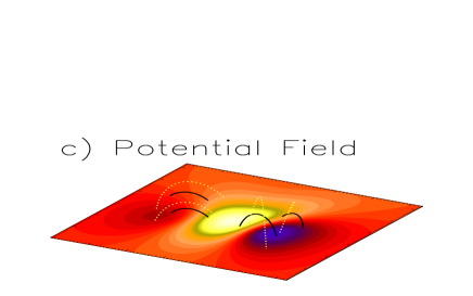
The potential field (lower left panel of Figure 4) produces quite high values of and the distances between projected field lines and loops are mostly larger than or . The potential magnetic loops are not a good approximation for the reconstructed plasma loops due to the quite high values of and as visible in Figure 2 panel c). The reconstruction (black) and original (yellow) are obviously far apart.
The potential field yet produces a correct association of the loops. or in average . Let us also note the lowest incorrect associations here , which are only slightly larger than the correct associations. If the correct loop association might not be absolutely clear after this step. In such a situation a further step is necessary to associate all features in both images with each other.
-
5.
If step 4 does not provide a clear association of features in the two images we need to undertake a further step. Here we check which combination of association of features will give the lowest values of (best agreement). In principle one would restrict this analysis to critical loops, which cannot be associated clearly because for features there are possible combinations. For our test example we computed all possibilities 222If the number of loops in the two STEREO-images are different, say , we get possible permutations..
For every combination we compute the mean of the C-values. The combination with the lowest value of is the most likely one. With all three magnetic field models (potential, linear force-free, non-linear force-free) we get the correct association as the most likely one. The correspondent values of are presented in the upper part of table 1 (Example 1).
Table 1: Here we show for two examples how good the loops in both STEREO-images can be associated with each other for different magnetic field models. As we associate four loops in both images, there is a total number of possible combinations. Here we shown only the best (lowest value of ) three combinations. B-field model Example 1 NonLin FF Lin FF Potential Example 2 NonLin FF Lin FF Potential All three magnetic field models give the lowest value of to the correct loop association. The best magnetic field model (nonlinear force-free) gives also the clearest answer regarding the optimal loop association. C for the optimal combination is a factor of lower than the second best combination. For linear force-free fields the best combination is still a factor of almost better than the second best. For potential field the second best combination is only about a factor of higher than the best one. This might still be enough to get some evidence about the correct association of loops in the two STEREO images. For the application to observational data one might include a threshold, e.g., consider only loops as clearly associated which each other when (the pairwise) value of C is lower than a certain threshold (say e.g., ). Larger values of might be in particular problematic if the loops or features are closer together then here. We apply our method to such a case in section 3.1.
-
6.
As the last step we do a geometric stereoscopic reconstruction, similar as described in section 2.1, but now with the knowledge which pairs of loops in the two images have to be used for the stereoscopic reconstruction. This knowledge removes already most of the ambiguities (visible as ghosts in Figure 2 b).
But even if we have identified pairs of loops in the two images this does not mean that we can identify each pixel along two associated curves in both images with each other. Consequently there can still be multiple points of intersection (and thus not a unique solution of the 3D reconstruction). Again, the magnetic field proxy (but now in 3D) can help here to resolve the ambiguity. From multiple point of intersection we chose that point, which has the closest distance to the magnetic field proxy. Even if we use a less than optimum magnetic field model we get a very good geometric stereoscopic reconstruction as seen in Figure 2 f) where a potential field has been used to remove the ambiguities of multiple intersection points. All stereoscopic reconstructed points (black) coincide with points of the original loops (yellow dotted). The ghost points (Figure 2 b) have vanished. One can see that the combination of geometric stereoscopy and magnetic modelling in Figure 2 f) is much more powerful than pure stereoscopy (Figure 2 b) or potential field magnetic modelling (Figure 2 c) alone. We call this combination of geometric (or ordinary) stereoscopy with magnetic modelling magnetic stereoscopy.
3.1 Example 2
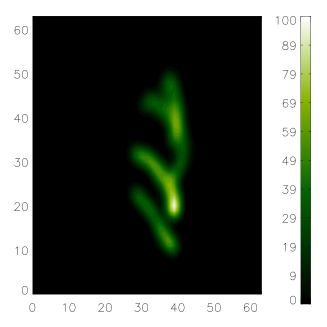
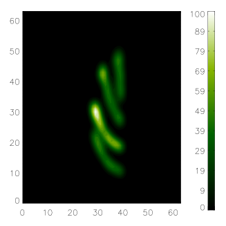
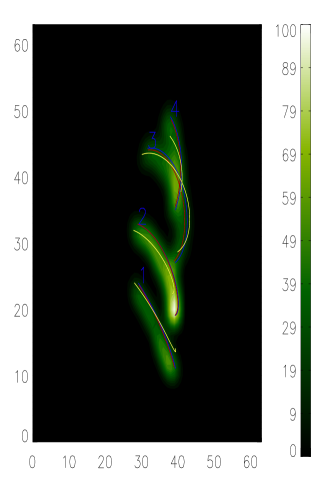
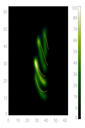

As a second example we apply our method to a set of loops that are closer together. The upper panel of Figure 5 shows two artificial EUV-images from different viewpoints (STEREO-1 and STEREO-2 in the right and left panel, respectively). The center column shows the structures enlarged and we overplot the image with different loops. The original loops are shown in blue and the projection of the nonlinear force-free field lines in red. As one can see the difference is very small. For loop-1 and 2 the red (nonlinear force-free) and blue (original) lines can hardly be distinguished in the right hand (STEREO-2) image. The projected images of the linear force-free field (yellow) are somewhat apart from the original.
Table 1 lower part (Example 2) shows the quantitative measures (average value of as explained in the last section) for the optimal loop association as well as for the second and third best combination. For a nonlinear force-free model the average distance is (as in example 1) less than of a pixel and this model gives the clearest answer regarding the correct association of loops as the second best loop association is a factor of worse then the correct one.
The linear force-free model provides a considerably higher value for the optimum combination of , which is, however, almost a factor of two better than the second best combination. Here (because we know the exact solution) we can also confirm that the optimum (lowest value of C) combination is the correct one. For real STEREO-data (where we do not know the correct solution of course) one has to trust merely on the values of C alone. The higher values of C for the linear force-free model tell us that this model is worse than the nonlinear force-free one. Here the linear force-free parameter was the same for all loops.
Similar as in example 1 the potential magnetic field gives the worst results. And here this model does not provide a clear association of the correct loops in both images to each other. Two combination (including the correct one) provide the same average value of C. We therefore conclude that a potential field is a too simple approximation.
In the left hand bottom panel of Figure 5 we show a pure geometric loop reconstruction (black) and the original loops in yellow. The reconstruction contains ghost features. In the bottom right hand panel we use magnetic stereoscopy, similar as described for the first example, but here based on a linear force-free model. Ambiguities (leading to ghost features) are removed by using the solution which is closest to the magnetic field model.
4 Conclusions
We describe a newly developed tool for the stereoscopic reconstruction of plasma loops from two images. The tool is intended to be used for the STEREO-mission. Within this work we tested the method with the help of a model active region, from which we computed images from two different viewpoints (artificial STEREO images). We tried to reconstruct the original 3D loops from the artificial images and compared the result with the original.
As a first step we tried a classical geometric stereoscopic reconstruction. The corresponding reconstruction contains ambiguities, because multiple points of intersection occur. As a consequence the reconstruction contains the correct 3D loops but also additional several so called ghost features. Within this approach we cannot distinguish between real and ghost features.
It is helpful, that the coronal plasma has a high conductivity and consequently the emitting plasma also outlines the coronal magnetic field. This means that a reconstruction of coronal loops is equivalent to the reconstruction of the magnetic field, e.g., a perfect magnetic field reconstruction would (if the correct, emitting magnetic field lines are chosen) also provide the plasma loops. Unfortunately it is hard to get the accurate coronal magnetic field and usually one has to extrapolate it from photospheric measurements with e.g., non-linear and linear force-free models or potential fields. We investigated how such coronal magnetic field models can be used to associate features in the two (artificial) STEREO-images. The method also provides us with a quantitative measure of the agreement between the magnetic field model and the observed loops. To do so we compute the average distances of the loops and the projections of magnetic field lines. If the distance measure is sufficiently small then the magnetic field model is already a good proxy of the 3D plasma loops. This is the ideal situation. As a result we not only get the 3D loops, but as well a reasonable coronal magnetic field model.
Due to noise, ambiguities and limited information (say if we only have line-of-sight magnetograms instead of vectormagnetograms) the plasma loops and magnetic loops (measured in both 2D projections) do not agree. In this case we obtain finite values of the measure and the magnetic field proxy is not a good (or perfect) approximation for the 3D plasma loop. The magnetic field proxy can help, however, to eliminate ambiguities in the geometric stereoscopic reconstruction. Firstly, the proxy helps to associate features in both images with each other and secondly if multiple intersection points still occur during the stereoscopy, we choose the point closest to the corresponding magnetic field line. Even an imperfect (or even an inconsistent one, e.g., different values of on different loops within the linear force-free approach) coronal magnetic field can be used for this aim.
As an outlook one might think about using the stereoscopic reconstructed plasma loops to improve the coronal magnetic field model.
Acknowledgements.
The work of Wiegelmann was supported by DLR-grant 50 OC 0501.Appendix A The model
We test our stereoscopic reconstruction tools with the help of an model active region. The advantage is here, that we know the exact solution and can check if our stereoscopy tools are able to find a reasonable reconstruction of the original.
We use the semi-analytic non-linear force-free field model developed by \inlinecitelow:etal90 as a model active region coronal magnetic field, with the parameters and . We compute this model active region in a computational box. To avoid (for the magnetic modelling tools) boundary effects we display only the center region in the 2D images (Figure 3) and the center 3D box (Figure 4).
We use the following spacecraft locations. STEREO-1 is somewhat below the ecliptic at and STEREO-2 is somewhat above the ecliptic at . The angle between the spacecraft is To compute artificial STEREO images from two different viewpoints we fill the magnetic field lines with plasma. To do so we use the scaling law which has been developed by \inlineciteschrijver:etal04 to compute artificial EUV images from a potential field magnetic field model. We used a somewhat modified approximation , where the magnetic field is in and the length in pixel. (An absolute scaling is not necessary here, because these data are only used to create the artificial STEREO images.)
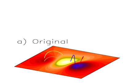
We show the 3D structure of four coronal loops in Figure 2 a). To compute a 3D density distribution we calculate a bundle of field lines for each loop, the center loop shown in Figure 2 a) and 11 more loops with footpoints located in a circle with the radius of pixel on the photosphere around the center loops. All loops are filled with plasma by the scaling law. Figure 3 shows two artificial images which mimic the different views of two STEREO-spacecraft. The artificial images have been taken with an angle of by a line-of-sight integration. The images show also the projection of the four center magnetic field lines.
References
- Amari, Boulmezaoud and Mikic (1999) Amari, T., Boulmezaoud, T.Z. and Mikic, Z.: 1999, Astron. Astrophys., 350, 1051.
- Aschwanden (2005) Aschwanden, M.J.: 2005, Solar Phys., 228, 339.
- Aschwanden et al. (1999) Aschwanden, M.J., Newmark, J.S., Delaboudinière, J.-P., Neupert, W.M., Klimchuk, J.A., Gary, G.A., Portier-Fozzani, F. and Zucker, A.: 1999, Astrophys. J., 515, 842.
- Aschwanden et al. (2000) Aschwanden, M.J., Alexander, D., Hurlburt, N., Newmark, J.S., Neupert, W.M., Klimchuk, J.A. and Gary, G.A.: 2000, Astrophys. J., 531, 1129.
- Batchelor (1994) Batchelor, D.: 1994, Solar Phys., 155, 57.
- Berton and Sakurai (1985) Berton, R. and Sakurai, T.: 1985, Solar Phys., 96, 93.
- Carcedo et al. (2003) Carcedo, L., Brown, D.S., Hood, A.W., Neukirch, T. and Wiegelmann, T.: 2003, Solar Phys., 218, 29.
- Chiu and Hilton (1977) Chiu, Y.T. and Hilton, H.H.: 1977, Astrophys. J., 212, 873.
- Gary, Davis and Moore (1998) Gary, G.A., Davis, J.M. and Moore, R.: 1998, Solar Phys., 183, 45.
- Inhester and Wiegelmann (2006) Inhester, B. and Wiegelmann, T.: 2006, Solar Phys., in press
- Lee, Newman and Gary (2006) Lee, J.K., Newman, T.S. and Gary, G.A.: 2006, Pattern Recognition, 39, 246.
- Low and Lou (1990) Low, B.C. and Lou, Y.Q.: 1990, Astrophys. J., 352, 343.
- Marsch, Wiegelmann and Xia (2004) Marsch, E., Wiegelmann, T. and Xia, L.D.: 2004, Astron. Astrophys., 428, 629.
- Portier-Fozzani and Inhester (2001) Portier-Fozzani, F. and Inhester, B.: 2001, Space Science Reviews, 97, 51.
- Régnier, Amari and Kersalé (2002) Régnier, S., Amari, T. and Kersalé, E.: 2002, Astron. Astrophys., 392, 1119.
- Sakurai (1981) Sakurai, T.: 1981, Solar Phys., 69, 343.
- Schmidt and Bothmer (1996) Schmidt, W.K.H. and Bothmer, V.: 1996, Adv. Space Res., 17, 369.
- Schrijver et al. (1999) Schrijver, C.J., Title, A.M., Berger, T.E., Fletcher, L., Hurlburt, N.E., Nightingale, R.W., Shine, R.A., Tarbell, T.D., Wolfson, J., Golub, L., Bookbinder, J.A., Deluca, E.E., McMullen, R.A., Warren, H.P., Kankelborg, C.C., Handy, B.N. and de Pontieu, B.: 1999, Solar Phys., 187, 261.
- Schrijver et al. (2004) Schrijver, C.J., Sandman, A.W., Aschwanden, M.J. and DeRosa, M.L.: 2004, Astrophys. J., 615, 512.
- Seehafer (1978) Seehafer, N.: 1978, Solar Phys., 58, 215.
- Semel (1967) Semel, M.: 1967, Annales d’Astrophysique, 30, 513.
- Valori, Kliem and Keppens (2005) Valori, G., Kliem, B. and Keppens, R.: 2005, Astron. Astrophys., 433, 335.
- Wheatland (2004) Wheatland, M.S.: 2004, Solar Phys., 222, 247.
- Wheatland, Sturrock and Roumeliotis (2000) Wheatland, M.S., Sturrock, P.A. and Roumeliotis, G.: 2000, Astrophys. J., 540, 1150.
- Wiegelmann (2004) Wiegelmann, T.: 2004, Solar Phys., 219, 87.
- Wiegelmann and Inhester (2003) Wiegelmann, T. and Inhester, B.: 2003, Solar Phys., 214, 287.
- Wiegelmann and Neukirch (2002) Wiegelmann, T. and Neukirch, T.: 2002, Solar Phys., 208, 233.
- Wiegelmann and Neukirch (2003) Wiegelmann, T. and Neukirch, T.: 2003, Nonlinear Processes in Geophysics, 10, 313.
- Wiegelmann, Inhester and Sakurai (2006) Wiegelmann, T., Inhester, B. and Sakurai, T.: 2006, Solar Phys., 233, 215.
- Wiegelmann et al. (2005a) Wiegelmann, T., Inhester, B., Lagg, A. and Solanki, S.K.: 2005a, Solar Phys., 228, 67.
- Wiegelmann et al. (2005b) Wiegelmann, T., Lagg, A., Solanki, S.K., Inhester, B. and Woch, J.: 2005b, Astron. Astrophys., 433, 701.
- Yan and Sakurai (2000) Yan, Y. and Sakurai, T.: 2000, Solar Phys., 195, 89.