Testing for monotonicity in the Hubble diagram

Abstract

General relativistic kinematics and the cosmological principle alone imply a monotonicity constraint in the Hubble diagram, which we confront to present-day supernova data. We use the running gradient method of statistical inference by Hall & Heckman (2000). We find no significant departure from monotonicity. The method seems well adapted and we recommend its use with future data.

1 Introduction

The Hubble diagram is one of the main pillars of modern cosmology. Indeed the accuracy in the measurement of apparent luminosity $\ell$ in Watt/m² and redshift $z$ of supernovae has dramatically increased in the last 20 years and is expected to continue so in the future. The theoretical understanding of the Hubble diagram remains a matter of lively discussion. A majority of view-points however accepts the kinematical assumptions of general relativity and the cosmological principle. These weak hypotheses are sufficient to produce a monotonicity constraint in the Hubble diagram of standard candles: in an open, expanding universe the apparent lumionosity is a decreasing function of distance and consequently of redshift. More stringently, the function $g(z):=(z+1)^{2}\ell(z)$ must be decreasing. The two factors $(z+1)$ come from the energy loss in the photon flux due to expansion induced redshift and surface increase. In a closed universe, the apparent luminosity may increase thanks to gravitational macro-lensing. The function $g(z)$ can go through at most one minimum as the photon goes over the equator. For higher $z$ then, $g(z)$ must be increasing. Its smallest observed value yields a lower bound for the radius of the universe. Our best experimental data today are the 137 supernovae of the ‘Gold’ sample compiled by Riess et al. (2004) [1] yielding a lower bound of $1.2\cdot 10^{26}$ m and a preliminary statistical analysis sees no sign of non-monotonicity in $g(z)$, Schücker & Tilquin (2006) [2].

The origins of order restricted statistical inference go back to the early 1950’s [3, 4] and the field continues to develop for natural reasons: many types of problems in the real world are concerned with monotonic functions. For example, the probability of a particular response may increase with the treatment level, the failure rate of a component may increase as it ages.

The purpose of this note is to apply the state of the art in testing monotonicity of a regression to the Hubble diagram. We choose the ‘running gradient’ type method by Hall & Heckmann (2000) [5], and develop a modification suitable to the closed universe case.

2 Methodology

Denote the data by $(z_{i},Y_{i},\sigma_{i})$, $i=1,\ldots,n$, where the redshifts $z_{i}$ are indexed in increasing order, $Y_{i}=\log_{10}g(z_{i})$ , and $\sigma_{i}$ is the standard deviation of the measurement $Y_{i}$.

The basic idea of a family of tests is the following: for a region $R(r,s)=[z_{r+1},z_{s}]$ with $s>r+1$, calculate a measure $T(r,s)$ of the departure from monotonicity of the relation of $Y_{i}$ and $z_{i}$, for $z_{i}\in R(r,s)$. The overall test statistic is $T=\sup_{r,s}T(r,s)$, where the supremum is taken over a predetermined set of pairs $(r,s)$. The test thus scans for deviations from monotonicity over a range of locations and scales. The p-value for the test is determined by comparing the observed value of $T$ to the distribution determined by simulation when monotonicity holds.

There are obviously a variety of constructions of this form; we use one proposed and analyzed in [5]. To test the null hypothesis that $g(z)$ is monotone versus any deviation from monontonicity the regions are of the form $[z_{r+1},z_{s}],~{}0\leq r\leq s-m\leq n-m$, where $m\geq 2$ is a parameter to be specified. To test versus the alternative that the $g(z)$ is non-monotone but with a single minimum, the regions are of the form $[z_{r+1},z_{n}]$. In each region the measure of departure from monotonicity is the slope of the weighted least squares line fit to the corresponding $(z,Y)$ pairs divided by its standard error. The weights are determined by the $\sigma_{i}$. The overall test statistic of the null hypothesis that the relationship is monotone decreasing versus the unconstrained alternative hypothesis that is it not is thus

$$T=\max_{0\leq r\leq s-m\leq n-m}T(r,s),$$ (1)

where $T(r,s)=\hat{b}(r,s)/\sigma_{\hat{b}(r,s)}$ with

$$\hat{b}(r,s) = \frac{\sum w_{i}Y_{i}(z_{i}-\bar{z}_{w})}{\sum w_{i}(z_{i}-\bar{z}_{w})^{2}},$$ (2)

$$\sigma_{\hat{b}(r,s)} = \left(\frac{1}{\sum w_{i}(z_{i}-\bar{z}_{w})^{2}}\right)^{1/2}.$$ (3)

Here the summation runs over $i=r+1,\ldots,s$, $w_{i}=1/\sigma_{i}^{2}$ and $\bar{z}_{w}=\sum w_{i}z_{i}/\sum w_{i}$. The constrained test is as above, but with $s=n$.

The significance of the test statistic $T$ is determined by simulation. We assume that the errors are Gaussian with mean zero and variances $\sigma_{i}^{2}$. In [5] it is shown that simulating under the model of a constant relationship provides p-values that are conservative, in the sense that if one were able to simulate from the true monotonically decreasing relationship, the p-value thus obtained would be stochastically smaller than the p-value obtained by simulating from a model in which the relationship was constant. It is also shown that the results are somewhat robust to deviations from the Gaussian model. One thus simulates from a model in which the $z_{i}$ are those in the actual data and the $Y_{i}$ are Gaussian with means zero and variances $\sigma_{i}^{2}$.

3 Numerical Results

Figure 1: All 137 ‘Gold’ samples of Riess et al. (2004), showing $Y_{i}=\log_{10}g(z_{i})$ as a function of $z_{i}$ for $i=1,\ldots,137$. Error bars show a range $\pm 2\sigma_{i}$ for each observation.

Figure 2: The regions with the largest deviation from monotonicity for the unconstrained test (left) and constrained test (right).

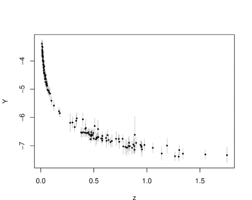
Assuming approximately normal distributed errors in the measurement of the distance modulus, the methodology of [5] can be applied to the ‘Gold’ sample by Riess et al. (2004). The data are shown in Figure 1. The 137 observations $i=1,\ldots,137$ consist of triplets $(z_{i},Y_{i},\sigma_{i})$, where $Y_{i}=\log_{10}g(z_{i})$ and $\sigma_{i}$ is the standard error of the observation of $Y_{i}=\log_{10}g(z_{i})$. As $Y_{i}$ is proportional to $-2\mu_{i}/5$, where $\mu_{i}$ is the observed distance modulus, the standard error $\sigma_{i}$ is given by the standard error of the observation of $\mu_{i}$ times $2/5$.

We choose a value of $m=6$, so that at least six observations fall into each considered interval (results are very insensitive to this choice).

3.1 No prior

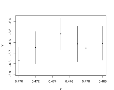
If the test statistic is calculated over all possible intervals, a stretch of observations between 0.47 and 0.495 attains the largest standardized slope of 1.677. This region is shown in the left panel of Figure 2. However, if assessing the significance of this result by 1000 simulations of the test statistic under the assumption of a constant $Y(z)$, all 1000 simulations yield a larger test statistic. The observations do therefore not represent a significant departure from a monotonically decreasing function $g$. For smaller values of $m$ than the chosen value $m=6$, the region with largest standardized slope contains the observations in the leftmost part of the region [0.47,0.495]. The obtained standardized slopes are, as for $m=6$, not even close to being a significant departure from monotonicity. The conclusion are thus insensitive to the choice of the minimal number of observations $m$ that have to fall within a region over which the standardized slope is calculated. A larger value of $m$ like the chosen $m=6$ has the advantage of being a more robust estimation procedure. If errors of the observations are in effect more heavy-tailed than a Gaussian distribution would suggest, results are more reliable for larger values of $m$, as the effect of an outlier in the data has less effect on the overall result if a larger number of observations are available for each interval over which the standardized slope is calculated. The compatibility of the observations with monotonicity and the location of the window of largest deviation are in agreement with the preliminary test in [2].

3.2 Assuming a closed universe

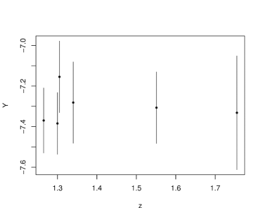
Let us suppose that the universe is closed and that its typical minimum of $g(z)$ is not hidden behind our horizon. Then deviations from monotonicity are to be expected for larger redshifts and it is natural to constrain the test to intervals including the observation with the largest value of $z=1.755$. The constrained test would be expected to be more powerful, since the maximum in (1) is taken over a smaller, targeted, set. The largest slope $\hat{b}$ is then obtained for a stretch of 6 observations between $z=1.265$ and the largest $z=1.755$, where one obtains a positive standardized slope of $T(n-7,n)\approx 0.0385$ and hence $T\approx 0.0385$. This region is shown in the right panel of Figure 2. The standardized slope is smaller than in the unconstrained test. However, if assessing the significance of this result by 1000 simulations of the test statistic under the assumption of constant $Y(z)$, a larger test statistic $T$ than the observed value 0.0385 was obtained for 973 runs. The result is therefore more significant than the unconstrained one, but still comfortably compatible with monotonicity.

4 Conclusion

Present-day supernova data are compatible with the monotonicity constraint in the Hubble diagram. Since this constraint is kinematical, i.e. independent of the presently debated issues related to inflation, dark energy or dark matter, it will be worthwhile to keep testing it as new data come in. For this purpose, a ‘running gradient’ type method like the one by P. Hall and N. Heckmann (2000) [5] used here seems well adapted for its flexibility and numerical ease of use.

Acknowledgements: Nicolai Meinshausen is supported by a fellowship of DFG (Deutsche Forschungsgemeinschaft); John Rice acknowledges the support of a grant from the US National Science Foundation, AST-0507254; Thomas Schücker acknowledges a research semester granted to him by his home institutes and thanks Vaughan Jones for his generous hospitality and coaching.

References

- [1] A. G. Riess et al., Type Ia supernova discoveries at , Astroph. J. 607 (2004) 665
- [2] T. Schücker, A. Tilquin, From Hubble diagrams to scale factors, Astron. Astrophys. 446 (2006) 413, astro-ph/0506457
- [3] R. Barlow, D. Barholomev, J.M. Brenner, D. Brunk, Statistical Inference Under Order Restrictions, Wiley, London (1972)
- [4] T. Robertson, F.F. Wright, R.L. Dykstra, Order Restricted Statistical Inference, Wiley, Chichester (1988)
- [5] P. Hall, N. Heckmann, Testing for monotonicity of a regression mean by calibrating for linear functions, Annals of Statistics 28 (2000) 20