Turbulent Mixing and the Dead Zone in Protostellar Disks

Abstract

We investigate the conditions for the presence of a magnetically inactive dead zone in protostellar disks, using 3-D shearing-box MHD calculations including vertical stratification, Ohmic resistivity and time-dependent ionization chemistry. Activity driven by the magnetorotational instability fills the whole thickness of the disk at 5 AU, provided cosmic ray ionization is present, small grains are absent and the gas-phase metal abundance is sufficiently high. At 1 AU the larger column density of 1700 g cm^-2 means the midplane is shielded from ionizing particles and remains magnetorotationally stable even under the most favorable conditions considered. Nevertheless the dead zone is effectively eliminated. Turbulence mixes free charges into the interior as they recombine, leading to a slight coupling of the midplane gas to the magnetic fields. Weak, large-scale radial fields diffuse to the midplane where they are sheared out to produce stronger azimuthal fields. The resulting midplane accretion stresses are just a few times less than in the surface layers on average.

1 INTRODUCTION

Turbulence plays a central role in protostellar disks. It transports orbital angular momentum, controlling the accretion of gas on the central star (Shakura & Sunyaev, 1973); brings dust grains together in the early stages of planet formation (Weidenschilling & Cuzzi, 1993); and modifies the orbital migration of protoplanets (Nelson & Papaloizou, 2004). Turbulence can be driven by the magneto-rotational instability (MRI; Balbus & Hawley 1991) in regions where the ionization is sufficient to couple the gas to the magnetic fields. The MRI operates by transferring orbital angular momentum outward along magnetic field lines linking gas on different orbits. The fastest linear growth rate is three-quarters the orbital frequency $\Omega$ and occurs at wavelengths near $\lambda_{c}=2\pi v_{A}/\Omega$ in fully-ionized Keplerian disks with Alfven speed $v_{A}$ (Balbus & Hawley, 1991). In the non-linear regime, the gravitational energy released from the inspiraling gas sustains turbulence and regenerates the magnetic fields (Balbus & Hawley, 1998). Good coupling of the fields to the gas within a few tenths of an AU of the star comes from thermal ionization of the low-ionization-potential elements potassium and sodium (Pneuman & Mitchell, 1965; Umebayashi, 1983). At greater distances, the ionization is due to the absorption of stellar X-rays or interstellar cosmic rays in the disk material. The X-rays penetrate to columns of about 10 g cm^-2 (Igea & Glassgold, 1999) and the cosmic rays to 100 g cm^-2, while recombination is generally fastest in the dense interior, leading to a layered structure. The top and bottom surfaces of the disk are magnetically active. The interior is quiescent and called the dead zone (Gammie, 1996). The dead zone is of special interest because it overlaps the region where the planets are found and potentially provides the environment and the raw ingredients for planet formation. The simplest layered picture, however, yields an accretion rate independent of stellar mass, conflicting with data for T Tauri stars. Including the extra heating from irradiation of the disk by the star gives a mass dependence that is still too weak (Hartmann et al., 2006), indicating that our understanding of the dead zone is incomplete.

The size of the dead zone depends on the disk surface density, the abundance of the dust that hastens recombination (Wardle & Ng, 1999; Sano et al., 2000), the presence of long-lived metal ions (Fromang et al., 2002) and the rate at which the turbulence mixes the charged species into the interior (Inutsuka & Sano, 2005; Ilgner & Nelson, 2006b). Well-mixed 0.1-$\mu$m grains with the interstellar dust-to-gas mass ratio in the minimum-mass Solar nebula produce a dead zone extending to about 20 AU (Sano et al., 2000; Matsumura & Pudritz, 2006). Even if small grains are absent, the annulus immediately outside the thermally-ionized region is quiescent for a wide range of disk models because the high surface densities mean cosmic rays and X-rays are absorbed before reaching the midplane. In this paper we investigate whether the dead zone can be eradicated under favorable conditions leaving the entire disk active. Because cosmic rays penetrate more deeply, their ionizing effects are included despite possible screening by the protostellar wind. Slow recombination is ensured by assuming the dust surface area per unit gas mass has declined through settling, coagulation and orbital evolution sufficiently that recombination on grain surfaces can be neglected. Since the abundance of gas-phase metal atoms is not well known, it is treated as a parameter. We focus on conditions near the present orbits of the Earth and Jupiter and use the minimum-mass Solar nebula (Hayashi et al., 1985) as the disk model. We extend results from Fleming & Stone (2003) by making stratified shearing-box MHD calculations including time-dependent ionization chemistry.

The paper has six sections. The ionization-recombination reaction network, disk model and MHD methods are described in section 2. The network is used in section 3 to estimate the size of the dead zone in local chemical equilibrium. Expansion or contraction of the dead zone through turbulent mixing is explored using MHD calculations in section 4 while section 5 deals with simple expressions for predicting the boundaries of the dead zone. A summary and conclusions are in section 6.

2 METHODS

2.1 Reaction Network

The ionization state of the disk gas is calculated using the simplified reaction network developed for molecular cloud studies by Oppenheimer & Dalgarno (1974). Five species are involved: molecular hydrogen and its ion; magnesium, a representative metal, and its ion; and free electrons. These take part in the four reactions

$${\rm H}_{2} \rightarrow {\rm H}_{2}^{+}+e^{-}$$ (1)

$${\rm H}_{2}^{+}+e^{-} \rightarrow {\rm H}_{2}$$ (2)

$${\rm H}_{2}^{+}+{\rm Mg} \rightarrow {\rm H}_{2}+{\rm Mg}^{+}$$ (3)

$${\rm Mg}^{+}+e^{-} \rightarrow {\rm Mg}+h\nu.$$ (4)

The ionization (eq. 1) is balanced by both dissociative recombination of the molecular ion (eq. 2) and molecule-metal charge exchange (eq. 3) followed by the radiative recombination of the metal ion (eq. 4). The rate coefficients are $3\times 10^{-6}/\sqrt{T}$ cm³ s^-1 for dissociative recombination, $3\times 10^{-9}$ cm³ s^-1 for charge exchange and $3\times 10^{-11}/\sqrt{T}$ cm³ s^-1 for radiative recombination at a temperature $T$ in Kelvin (Ilgner & Nelson, 2006a). Because radiative recombination is slowest, the positive charge typically resides on metal ions in chemical equilibrium. Comparison with a comprehensive network of almost 2000 reactions shows that the Oppenheimer & Dalgarno network yields slightly higher equilibrium electron abundances because fewer recombination pathways are included (Ilgner & Nelson, 2006a). A similar reduced reaction set adequately reproduces the ionization fraction from a detailed chemical model of the midplane of a protostellar disk at 1 AU (Semenov et al., 2004). The kinetic equations for the reactions 1-4 form a stiff set of ODEs that is integrated using semi-implicit extrapolation (Press et al., 1992). Solving the reaction network uses about ten times as many CPU cycles per zone as evolving the magnetic fields.

The cosmic ray ionization rate is reduced from the interstellar value $\zeta_{CR}=10^{-17}$ s^-1 (Caselli et al., 1998) by the shielding effects of the surrounding disk material. The total ionization rate

$$\zeta(z)={\zeta_{CR}\over 2}\left\{\exp\left[-\chi^{+}(z)\over\chi_{CR}\right]+\exp\left[-\chi^{-}(z)\over\chi_{CR}\right]\right\}$$ (5)

depends on the cosmic ray absorption depth $\chi_{CR}=96$ g cm^-2 and the column above and below the point of interest, $\chi^{+}=\int_{z}^{+\infty}\rho\,dz$ and $\chi^{-}=\int_{-\infty}^{z}\rho\,dz$. In the 3-D MHD calculations of section 4, the column densities are averaged over the horizontal extent of the domain when finding the ionization rate.

The resistivity is computed from the electron abundance by

$$\eta=234\,{\sqrt{T}\over x_{e}}\,{\rm cm^{2}s^{-1}},$$ (6)

where $x_{e}=n_{e}/n_{n}$ is the electron fraction, $n_{e}$ the electron number density and $n_{n}$ the total number density of neutrals (Blaes & Balbus, 1994).

2.2 Disk Model

Our model disk is the minimum-mass Solar nebula in which the surface density and temperature vary with radius $r$ as $\Sigma=1700(r/{\rm AU})^{-3/2}$ g cm^-2 and $T=280(r/{\rm AU})^{-1/2}$ K, respectively. The temperature is independent of the distance from the midplane, so that in hydrostatic equilibrium the density falls off with height $z$ as $\exp(-z^{2}/2H^{2})$. The scale height $H=c_{s}/\Omega$ depends on the sound speed $c_{s}=({\cal R}_{gas}T/\mu)^{1/2}$.

The composition of the material is Solar (Asplund et al., 2005), with 0.085 helium and $3.39\times 10^{-5}$ magnesium atoms per hydrogen nucleus. The hydrogen is molecular and the mean molar weight $\mu=2.29$. Only gas-phase magnesium contributes to the overall ionization level, while the magnesium atoms can take three forms, (1) incorporated into silicate and metallic grains, (2) adsorbed on grain surfaces and (3) in the gas phase. Measurements of the diffuse interstellar gas show that about half the magnesium is in grains (Sofia, Cardelli & Savage, 1994; Fitzpatrick, 1997). We assume the remainder is divided between grain surfaces and the gas phase through thermal adsorption and desorption and we calculate the equilibrium gas-phase fraction as outlined by Ilgner & Nelson (2006a). The equilibrium is reached quickly, as the lifetime of adsorbed magnesium atoms is just $10^{-4}$ seconds at 1 AU and 280 K, or $10^{6}$ seconds at 5 AU and 125 K. Almost all the magnesium not in grain interiors is in the gas phase at 1 AU, while at 5 AU just 1.4% stays in the gas if 0.1-micron grains are present with the interstellar mass fraction. If the gas-phase magnesium abundance is unchanged by the removal of the small grains, its most probable value is half Solar at 1 AU and 0.7% Solar at 5 AU. We consider a range of possible magnesium abundances below.

The evolution of the magnetic fields is potentially affected by the Ohmic, Hall and ambipolar diffusion terms in the induction equation. We estimate the magnitudes of the terms as outlined in Sano & Stone (2002a). The Ohmic and Hall terms are comparable near the midplane, while the ambipolar term is the largest of the three only above about $3H$. Linear analyses (Wardle, 1999; Balbus & Terquem, 2001; Salmeron & Wardle, 2005) indicate the Hall term has little effect on the maximum MRI growth rate but extends the range of unstable wavelengths. Numerical results suggest the strength of the saturated turbulence is largely unaffected by the Hall term and is determined by the Ohmic term (Sano & Stone, 2002b). The ambipolar term decouples the neutral gas from the ionized component (Hawley & Stone, 1998) at the low densities found in our model disk outside $|z|=4H$, where collisions transfer momentum from the ions to the neutrals at rates less than the orbital frequency. Little accretion of neutral gas due to MRI turbulence will occur beyond four scale heights. Since the Ohmic term is most important for the size of the dead zone, we choose to focus on the effects of the Ohmic resistivity.

2.3 MHD Equations

The standard equations of resistive MHD,

$${{\partial\rho}\over{\partial t}}+{\bf\nabla\cdot}(\rho{\bf v})=0,$$ (7)

$${{\partial{\bf v}}\over{\partial t}}+{\bf v\cdot\nabla v}=-{{\bf\nabla}p\over\rho}+{1\over 4\pi\rho}({\bf\nabla\times B}){\bf\times B}-2{\bf\Omega\times v}+3\Omega^{2}{\bf\hat{x}}-\Omega^{2}{\bf\hat{z}},$$ (8)

and

$${\partial{\bf B}\over\partial t}={\bf\nabla\times}({\bf v\times B}-\eta{\bf\nabla\times B}),$$ (9)

are solved with an isothermal equation of state $p=\rho c_{s}^{2}$, using the ZEUS code (Stone & Norman, 1992a, b). When the chemical reactions are included, an additional continuity equation

$${{\partial\rho_{i}}\over{\partial t}}+{\bf\nabla\cdot}(\rho_{i}{\bf v})=0,$$ (10)

is solved for each of the five chemical species $i$. The domain is a three-dimensional shearing-box (Hawley, Gammie, & Balbus, 1995) and vertical stratification is included. The radial or $x$-boundaries are periodic, with an azimuthal offset that increases in time according to the radial gradient in orbital speed. The azimuthal or $y$-boundaries are strictly periodic, while the vertical or $z$-boundaries allow outflow but no inflow. The domain extends two density scale heights $H$ along the radial direction, eight along the orbital direction and four either side of the midplane and is divided into $32\times 64\times 128$ grid zones. Short timesteps are avoided by applying a density floor of $1/15$ the minimum initial density. The floor typically operates in just a few grid zones near domain top and bottom, and for all the calculations described in this paper the mass added is much less than the mass escaping through the boundaries, which in turn is in most cases less than 1% of the total initial mass per 30 orbits. The starting magnetic field has strength $B_{0}$ chosen so that the midplane MRI wavelength is $0.5H$. The components of the field are $(B_{x},B_{y},B_{z})=[0,B_{0}\sin(\pi x/H),B_{0}\cos(\pi x/H)]$. Magnetic pressure and tension forces initially vanish, as the field strength is uniform and the field lines are straight. The net magnetic flux is zero because the field lines rotate $360^{\circ}$ round the $y-z$ plane across the radial extent of the box. Due to the periodic conditions on the side boundaries, the vertical component of the magnetic flux is conserved during the calculations. The outflow conditions on the top and bottom boundaries mean that, unlike the calculations discussed by Fleming & Stone (2003), the radial and azimuthal magnetic fluxes are free to evolve over time.

3 TIMESCALES

To gain an overall grasp of the problem, we estimate three timescales affecting the size of the dead zone. These are (1) the Ohmic dissipation time for the magnetic fields, (2) the turbulent mixing time and (3) the time for ionized gas to recombine and reach chemical equilibrium. The dead zone is the region where the magnetic fields dissipate too fast for the MRI to grow. The dissipation time is calculated in this section assuming local chemical equilibrium so that the electron abundance at each height results solely from local ionization and recombination processes. However the dead zone boundaries will shift if ionized gas from the surface layers is mixed to the interior before recombining. The three corresponding timescales are calculated as follows.

1. Like any diffusion timescale, the dissipation and mixing times are ratios of a squared length to a diffusion coefficient. The diffusion coefficient $\eta$ for resistive dissipation is given by eq. 6. For the length we choose the scale height $H$, yielding an upper bound on the dissipation time in the disk interior, where the magnetic fields can alternate in sign over distances shorter than the scale height. MRI turbulence is expected when the dissipation time is longer than the growth time of the instability. For example if the characteristic unstable wavelength $\lambda_{c}$ is one-tenth of the scale height then turbulence requires a dissipation time, $H^{2}/\eta$, longer than about $(0.1)^{-2}=100$ orbits. The diffusion time in orbits can be converted to a magnetic Reynolds number $c_{s}^{2}/(\eta\Omega)$ by multiplying by $2\pi$.

2. The mixing time depends on the turbulent diffusion coefficient, which is the product of the mean squared velocity fluctuation and the eddy correlation time (Fromang & Papaloizou, 2006). For a preliminary estimate of the mixing time, these quantities are taken from ideal-MHD shearing-box calculations, with the Ohmic resistivity switched off in eq. 9.

3. The recombination time is measured in the hydrostatic model disk starting with the magnesium and electron abundances equal, the magnesium fully-ionized and the molecular hydrogen neutral. The reaction network is then integrated until the electron abundance reaches equilibrium.

We consider conditions at 1 and 5 AU in the minimum-mass Solar nebula. The mixing times are found using turbulent diffusion coefficients from the ideal-MHD calculations M1 and M5 listed in table 1. The coefficients are averaged over the horizontal extent of the domain and over a period from 10 to 100 orbits after the turbulence is well-established.

Table 1: Calculation Parameters

Label	Physics	$R/{\rm AU}$	$x_{\rm Mg}/{\rm Solar}$	Duration/orbits
M1	Ideal MHD	1	–	100
F1	Fixed $\eta(z)$	1	1	150
V1	Varying $\eta(x,y,z,t)$	1	1	150
M5	Ideal MHD	5	–	100
F52	Fixed $\eta(z)$	5	$10^{-2}$	100
F56	Fixed $\eta(z)$	5	$10^{-6}$	100
F58	Fixed $\eta(z)$	5	$10^{-8}$	100

3.1 Timescales at 1 AU

Results for 1 AU are shown in figure 1. Because we aim to find the size of the active region under the most favorable conditions, we assume here that the gas-phase magnesium abundance is Solar. Nevertheless the magnetic fields dissipate in just three orbits at the midplane if the ionization is in equilibrium. The MRI is absent near $z=0$ as all modes fitting in the disk thickness (Sano & Miyama, 1999) are damped. The recombination time is several hundred years at the midplane and also at four scale heights, but is only thirty years at two scale heights, where the absolute number density of free electrons is greatest. At all heights, the turbulent mixing from the ideal-MHD calculation is faster than the recombination, suggesting mixing could affect the size of the dead zone.

Figure 1: Timescales for Ohmic dissipation (dotted), recombination (dashed) and turbulent mixing (solid) as functions of height at 1 AU, assuming Solar abundance for magnesium in the gas phase. The mixing timescale is taken from the ideal-MHD calculation M1.

The recombination and dissipation times depend on the metal abundance as shown in figure 2. The midplane Ohmic dissipation time is 3 orbits or less across the entire range of abundances considered, indicating that changes in the metal abundance alone will not remove the dead zone. In contrast, at $z=2H$ the dissipation time is longer than 100 orbits and magnetic activity is expected if the magnesium abundance is greater than $10^{-5}$ Solar. The dissipation and recombination times at all heights are abundance-independent above $10^{-4}$ Solar, so the results with Solar magnesium accurately reflect conditions throughout the likely abundance range: in local chemical equilibrium, the surface layers are magnetically active while the midplane is dead.

Figure 2: Midplane charged particle abundances (top panel) and timescales (bottom) versus gas-phase magnesium abundance at 1 AU. Above, H${}_{2}^{+}$ is shown by a long-dash-dotted line, Mg⁺ by a short-dash-dotted line and electrons by small circles. Below, the recombination timescale is shown by a dashed line and the Ohmic dissipation time per scale height by a dotted line. Circles near the left-hand edge mark the values when magnesium is absent.

3.2 Timescales at 5 AU

Figure 3 shows the height dependence of the timescales at 5 AU. The assumed gas-phase magnesium abundance is 1% of Solar, near the equilibrium value for thermal adsorption and desorption (section 2.2). MRI turbulence is expected at all heights because the dissipation is slow. The relatively high midplane electron fraction $x_{e}=6\times 10^{-10}$ is due to faster ionization than at 1 AU: cosmic rays reaching $z=0$ pass through a column of just 76 g cm^-2. The turbulent mixing is slower than the recombination in the interior, so the ionization profile will be unaffected by mixing. Midplane magnesium abundances greater than $10^{-6}$ Solar yield dissipation slow enough to permit the MRI to develop (figure 4).

Figure 3: Timescales for Ohmic dissipation (dotted), recombination (dashed) and turbulent mixing (solid), as functions of height at 5 AU, with a gas phase magnesium abundance $10^{-2}$ Solar. The mixing timescale is taken from the ideal-MHD calculation M5.

Figure 4: Midplane charged particle abundances (top panel) and timescales (bottom) versus gas-phase magnesium abundance at 5 AU. Symbols are as in figure 2: above, H${}_{2}^{+}$ is shown by a long-dash-dotted line, Mg⁺ by a short-dash-dotted line and electrons by small circles. Below, the recombination timescale is shown by a dashed line and the Ohmic dissipation time per scale height by a dotted line. Circles near the left-hand edge mark the values when magnesium is absent.

4 MAGNETIC ACTIVITY

According to the timescale estimates in section 3, layered accretion is expected at 1 AU, but turbulent mixing could be fast enough to reduce or dispense with the midplane dead layer. At 5 AU, the whole thickness of the disk will be active. Here we explore the magnetic activity using resistive MHD calculations with and without time-dependent ionization.

4.1 Turbulent Mixing at 1 AU

In calculation F1 the resistivity is a fixed function of height taken from the equilibrium ionization state in the initial hydrostatic disk model. The resulting flow has active surface layers and a midplane dead zone (figure 5). The stresses in the active layers are due mostly to magnetic forces, with the contribution from gas pressure gradients three to six times smaller, while at the midplane the total stress is an order of magnitude weaker and the magnetic and hydrodynamic parts are almost equal. The midplane magnetic stresses result from net radial and azimuthal fluxes that build up as fields of the opposing signs escape through the open vertical boundaries. Similar calculations by Fleming & Stone (2003) showed still weaker midplane magnetic stresses because the vertical boundaries were periodic or impermeable and the net radial magnetic flux remained zero. Like Fleming & Stone (2003) we observe hydrodynamic stresses in the dead zone due to sound waves propagating away from the active layers.

Figure 5: Mean accretion stress versus height in MHD calculations centered at 1 AU. The magnetic stress $-B_{x}B_{y}/4\pi$ is shown by solid lines, the hydrodynamic stress $\rho v_{x}\delta v_{y}$ by dotted lines; $\delta v_{y}$ is the azimuthal velocity relative to the background shear flow. The four panels show results from an ideal MHD run (top left), a resistive case with a fixed resistivity profile $\eta(z)$ (top right), and early and late stages from a run with time-varying resistivity (bottom left and right, respectively). The early results are averaged from 10 to 60 years, the late results from 100 to 150 years. The gas-phase magnesium abundance is Solar.

In run V1 the reaction network is solved together with the MHD equations. Electrons and ions are carried from place to place in the flow and the resistivity varies with all three space coordinates and time. For the first 60 years the flow again consists of active surface layers and a midplane dead zone (figures 5 and 6). The magnetic fields are weaker overall than the ideal-MHD case M1, leading to slower mixing. Recombination is faster than mixing within two scale heights of the midplane (figure 7), so the resistivity approaches its equilibrium profile from figure 1 even when the time-dependent chemistry is included. The dissipation time differs most from figure 1 in the active layers, where mixing makes the electron fraction and resistivity more nearly uniform. The turbulent mixing has little effect on the size of the midplane dead zone.

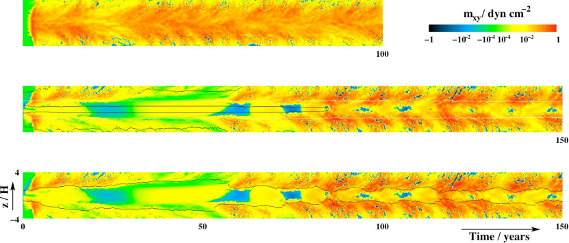
Figure 6: Horizontally-averaged magnetic accretion stress versus height and time at 1 AU in the ideal MHD calculation M1 (top panel) and the resistive MHD version with time-dependent chemistry V1 (two lower panels). The pair of black curves nearest the midplane in the middle panel shows where the magnetic Reynolds number $Re=c_{s}^{2}/(\eta\Omega)=100$, the white lines $Re=1000$ and the outer black curves $Re=10^{4}$. Black curves in the bottom panel mark where the Lundquist number $Lu=v_{Az}^{2}/(\eta\Omega)$ is unity. The common color scale is double logarithmic, with reds for positive stresses, blues for negative stresses and green for stresses within $10^{-4}$ dyn cm^-2 of zero.

Figure 7: Timescales for Ohmic dissipation (dotted), recombination (dashed) and turbulent mixing (solid) versus height at 1 AU in the MHD calculation V1 with time-dependent ionization. The results are averaged from 10 to 60 years (top panel) and from 100 to 150 years (bottom panel).

The situation changes around 60 years, when a period of stronger turbulence leads to faster mixing. Ionization at the midplane increases and the active regions expand toward $z=0$. The midplane electron fraction peaks at 87 years at $x_{e}=1.2\times 10^{-11}$ and then varies around $10^{-11}$ till the run ends at 150 years. The flow settles into a new state in which the mixing at the midplane is faster than the recombination, but still slower than the dissipation of magnetic fields (figure 7). The fast-growing MRI modes are adequately spatially resolved throughout the volume. Outside two scale heights the characteristic wavelength averages ten or more grid zones in the vertical direction due to the large Alfven speeds, while nearer the midplane the linear modes not damped by the resistivity have vertical wavelengths six zones or greater. The mean accretion stresses are similar to the ideal-MHD calculation M1 in the surface layers outside $|z|=H$, but a few times weaker at the midplane (figure 5). The midplane is magnetized and has a significant total accretion stress that is 0.2% of the local gas pressure. However the magnetic activity differs in character from the surface layers and is also unlike the midplane in the ideal-MHD run M1 in several respects:

1. The magnetic field shows few features smaller than a quarter of a scale height, as expected from the dissipation timescale of 20 years per scale height.

2. The magnetic stress $m_{xy}=-B_{x}B_{y}/4\pi$ is due mostly to large-scale fields, similar to the dead zone during the early part of the calculation, rather than small-scale fields as in the ideal-MHD run (figure 8). The horizontally-averaged magnetic stress $\left<m_{xy}\right>$ roughly equals the stress from the horizontally-averaged fields, $-\left<B_{x}\right>\left<B_{y}\right>/4\pi$, except for two periods of a few orbits around 87 and 117 years.

3. The horizontally-averaged stress varies around zero, while in the ideal-MHD case it is strictly positive (figure 8).

4. The mean ratio of magnetic to hydrodynamic stresses is just 1.9, intermediate between the ratios in the dead zone and active layers during the early part of the calculation.

5. The mean midplane pressure in the vertical component of the magnetic field is 125 times smaller than that in the azimuthal component, contrasting with the ratios around 30 found in run M1 and also typical of past MRI turbulence calculations (Miller & Stone, 2000). The relative strength of the azimuthal field suggests a generation mechanism distinct from the MRI.

6. The mean azimuthal magnetic field evolves mostly through shear acting on the mean radial field. If shear were the only effect, the azimuthal field at a time $t>t_{0}$ would be

   $$B_{y}^{sh}(t)=B_{y}(t_{0})-\int_{t_{0}}^{t}\frac{3}{2}\Omega B_{x}\,dt.$$ (11)

   The mean azimuthal field is plotted together with $B_{y}^{sh}$ in figure 9. The departure from the shear curve is shown over 20-year intervals by performing the integration from $t_{0}=0$ up to 10 years, from $t_{0}=10$ up to 30 years, from $t_{0}=30$ up to 50 years and so on. The field closely tracks the variation expected from shear throughout run V1, while the two curves are more weakly correlated in the ideal-MHD version M1.

These results indicate the magnetic fields evolve as follows. The fields delivered to the interior suffer Ohmic dissipation of small-scale structures, leaving a weak, almost uniform net radial component. Although the MRI is ineffective near the midplane due to the large resistivity, the shear produces a net azimuthal field, leading to an accretion stress that can be positive or negative. However the stress is negative for only short periods and when time-averaged is positive, driving accretion (figure 5). The shear-generated fields are expelled both up and down, leading to correlated activity in the two surface layers unlike run M1 (figure 6). The stresses and the azimuthal field strength peak about every ten orbits. Azimuthal field variations with similar periods occurred in MHD calculations by Brandenburg & Donner (1997). The variations depend little on the domain height provided the box extends to levels where the magnetic pressure exceeds the gas pressure, according to ideal MHD tests (Turner et al., 2006). Occasionally when the midplane azimuthal field is strongest it erupts, leading to the production of a large midplane radial field as at 87 and 117 years, and then is destroyed within a few orbits (figure 9). The magnetic energy dissipated in these outbursts per unit area per unit time is comparable to the radiative flux from the surface of the viscous model disk with the same stress and mass column, suggesting such events could be directly observed.

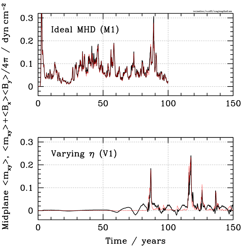
Figure 8: Midplane magnetic accretion stresses at 1 AU in the ideal MHD calculation M1 (top panel) and the resistive MHD calculation V1 (bottom panel). Stresses due to the entire magnetic field are shown by thick curves, those due to small-scale fields alone by thin red curves.

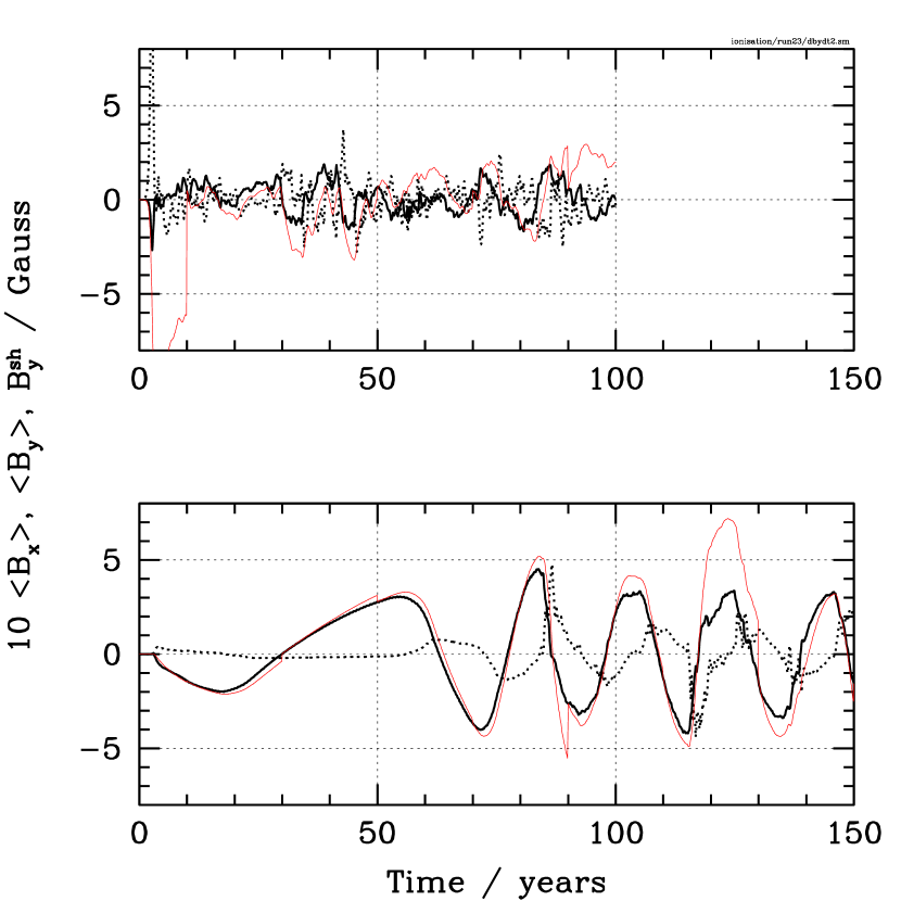
Figure 9: Midplane magnetic fields versus time at 1 AU in the ideal MHD calculation M1 (top panel) and the resistive MHD calculation V1 (bottom panel). The azimuthal component is shown by thick solid curves, the radial component by dotted curves. Both are horizontally-averaged and the radial component is multiplied by ten so its variations can be read on the same scale. The azimuthal field that would result from shear acting on the radial field (eq. 11) is indicated by thin red curves.

4.2 Turbulence at 5 AU

Turbulence fills the entire disk thickness in the shearing-box calculations at 5 AU that have gas-phase magnesium abundances $10^{-6}$ Solar and greater. No dead zone is present and the accretion stresses have almost identical mean vertical profiles in the cases M5, F52 and F56 (figure 10). By contrast, the run F58 with magnesium abundance $10^{-8}$ Solar has a dead zone extending two scale heights from the midplane. The midplane magnetic dissipation time per scale height in F58 is just 34 orbits, compared with 630 orbits in run F56 (figure 4). Recombination at the midplane takes only three orbits and is much faster than even the mixing in the ideal MHD run (figure 3), so turbulent mixing will not expunge the dead zone in this case.

Figure 10: Mean accretion stress versus height in four MHD calculations centered at 5 AU. The magnetic stress is shown by solid lines, the hydrodynamic stress by dotted lines. The four panels show results from an ideal MHD calculation (top left) and calculations with a fixed resistivity profile and gas-phase magnesium abundances 0.01 (top right), $10^{-6}$ (bottom left) and $10^{-8}$ times Solar (bottom right). The results are averaged from 10 to 100 orbits.

5 ACTIVITY CRITERIA

Simple criteria for the presence of turbulence driven by the MRI are extremely useful in developing protostellar disk models without the investment of time needed for three-dimensional MHD calculations. Two such criteria are tested in this section.

An Ohmic resistivity quenches the linear growth of the MRI if the magnetic fields diffuse across the characteristic wavelength $\lambda_{c}$ faster than the perturbations grow. The diffusion time is the wavelength squared divided by the resistivity, yielding a criterion for instability on vertical fields

$$Lu\equiv{v_{Az}^{2}\over\eta\Omega}>1$$ (12)

in agreement with linear analyses (Jin, 1996; Sano & Miyama, 1999). The left-hand side of eq. 12 is the dimensionless Lundquist number. In the fully-developed turbulence, the growth is most easily halted by diffusion perpendicular to the midplane because on average the field reverses direction most often per unit length along the $z$-direction. Numerical unstratified shearing-box results indicate that eq. 12 applies to the turbulence also (Sano & Inutsuka, 2001; Sano & Stone, 2002b).

The second activity criterion is constructed using the diffusion time across the density scale height $H$. The resulting magnetic Reynolds number $Re\equiv c_{s}^{2}/(\eta\Omega)$ is independent of the field strength and so the value required for instability depends on the fields present. Turbulence occurred only at Reynolds numbers greater than $10^{4}$ with zero net magnetic flux and at Reynolds numbers as low as 100 with a net vertical magnetic flux, in unstratified shearing-box calculations by Fleming et al. (2000).

The edges of the dead zone according to the two activity criteria are shown in figure 6. In run V1 with the reaction network, the Reynolds number is less than $10^{4}$ throughout the domain after about 60 years and greater than 100 everywhere from 85 years on. By the zero net flux criterion $Re>10^{4}$ the dead zone fills the domain, which is clearly not the case. On the other hand by the vertical field criterion $Re>100$, the dead zone is completely absent and MRI activity extends to the midplane, contradicting the evidence outlined in section 4.1. It may be that neither of these criteria applies to our calculations, which have zero net vertical but non-zero net radial and azimuthal magnetic fluxes. An intermediate critical Reynolds number of 1000, corresponding to a dissipation time of 160 orbits per scale height, more nearly approximates the boundaries of the MRI active regions, but fails to respond to the changes in magnetic field strength over the course of the calculation. In contrast to these three possible critical Reynolds numbers, as shown in the bottom panel of figure 6 a Lundquist number unity accurately traces the edges of the MRI turbulent layers at all times in run V1.

The activity criteria are similar at 5 AU. The mean midplane Reynolds number is $6\times 10^{4}$ in run F52, 4000 in run F56 and 200 in run F58. Only the last of these has a dead zone (figure 10), consistent with a critical Reynolds number of 1000 for this situation. The Lundquist number is greater than unity at all heights in the first two cases and greater than unity in run F58 only outside the MRI dead zone, again obeying eq. 12.

Overall, the Reynolds number suffers from the difficulty that its critical value must be determined for each magnetic field configuration using 3-D MHD calculations, while the Lundquist number always has a critical value unity. The Lundquist criterion is preferable because it explicitly shows the magnetic field dependence. Neither dimensionless number bypasses the basic uncertainty regarding the net magnetic flux, which is an input parameter for the shearing box calculations. However once a disk model and field are chosen, the Lundquist criterion eq. 12 immediately gives the size of the dead zone.

6 CONCLUSIONS

We investigated whether the dead zone is eliminated from the minimum-mass Solar nebula under favorable conditions. Cosmic rays are assumed to reach the disk surface, recombination on grains is absent and metals are found in the gas phase. The most restrictive of these assumptions is the lack of small grains. Particles 0.1 $\mu$m in radius can significantly affect the thickness of the dead zone at 1 AU even with dust-to-gas mass ratios 100 times lower than the interstellar value (Sano et al., 2000). The gas-phase metal abundance is a less important parameter and can be several orders of magnitude below its nominal value with little change in the dead zone size.

Timescale estimates and numerical resistive MHD calculations both show that the whole of the disk thickness at 5 AU is active if the gas-phase magnesium abundance is greater than $10^{-6}$ times Solar, consistent with results at a similar column density from Ilgner & Nelson (2006a). The problem is more severe at 1 AU, where few ionizing particles penetrate to the midplane if the column density is 1700 g cm^-2. In chemical equilibrium the dead zone thickness declines with increasing gas-phase magnesium abundance but asymptotes at values above $10^{-4}$ times Solar with most of the mass column still magnetically inactive. However ionized gas can reach the interior through turbulent mixing, because the recombination and mixing timescales are similar. In an MHD calculation including time-dependent ionization chemistry, free electrons arrive at the midplane fast enough to maintain a weak coupling to the magnetic fields. The midplane remains linearly stable against the MRI because of the large resistivity, but receives magnetic fields generated in the surface layers. The midplane fields are smooth while those in the surface layers are tangled. The boundary between the two lies at the height where the MRI is marginally stable and the Lundquist number is unity. Radial fields of one sign preferentially escape from the disk surfaces, leaving the midplane with a net radial magnetic flux of the opposite sign and leading to the generation of azimuthal fields through shear. The resulting accretion stress varies around zero, but on average is positive and just a few times less than the stress in the active layers.

These results demonstrate that the dead zone can be eradicated and the midplane gas flow toward the star even if the MRI occurs only in the surface layers. Magnetic forces can provide angular momentum transfer throughout the planet formation region once small grains have been removed. However the midplane flow at 1 AU is fundamentally different from the usual picture. It is magnetorotationally stable and has magnetic stresses that are uniform on scales up to the disk thickness. The presence of internal stresses yields a greater overall accretion rate than the basic layered model, permitting a stronger dependence on the stellar mass as required by brown dwarf and T Tauri star measurements (Hartmann et al., 2006). Time variability in our calculations is due to fluctuations in the magnetic field strength. Longer-period accretion variability can arise from the pileup of material reaching the dead zone, even in the presence of midplane stresses (Wünsch et al., 2006); these effects are not included in our calculations. The smooth internal magnetic fields have pressures up to 5% of the gas pressure and are strong enough to modify the orbital migration of Earth-mass protoplanets through their effects on the corotation resonance (Terquem, 2003). Other potentially important effects in the dead zone are the transport of magnetic flux over large radial distances and the interactions between disk annuli carrying opposing magnetic fields. These can be explored with future global MHD calculations.

References

- Asplund et al. (2005) Asplund, M., Grevesse, N., & Sauval, A. J. 2005, in “Cosmic Abundances as Records of Stellar Evolution and Nucleosynthesis”, ASP Conf. Ser., vol. 336, ed. T. G. Barnes III & F. N. Bash (San Francisco: Astronomical Society of the Pacific), 25
- Balbus & Hawley (1991) Balbus, S. A., & Hawley, J. F. 1991, ApJ, 376, 214
- Balbus & Hawley (1998) Balbus, S. A., & Hawley, J. F. 1998, Rev. Mod. Phys., 70, 1
- Balbus & Terquem (2001) Balbus, S. A., & Terquem, C. 2001, ApJ, 552, 235
- Blaes & Balbus (1994) Blaes, O. M., & Balbus, S. A. 1994, ApJ, 421, 163
- Brandenburg & Donner (1997) Brandenburg, A., & Donner, K. J. 1997, MNRAS, 288, L29
- Caselli et al. (1998) Caselli, P., Walmsley, C. M., Terzieva, R., & Herbst, E. 1998, ApJ, 499, 234
- Fitzpatrick (1997) Fitzpatrick, E. L. 1997, ApJ, 482, L199
- Fleming et al. (2000) Fleming, T., Stone, J. M., & Hawley, J. F. 2000, ApJ, 530, 464
- Fleming & Stone (2003) Fleming, T., & Stone, J. M. 2003, ApJ, 585, 908
- Fromang & Papaloizou (2006) Fromang, S., & Papaloizou, J. 2006, A&A, 452, 751
- Fromang et al. (2002) Fromang, S., Terquem, C., & Balbus, S. A. 2002, MNRAS, 329, 18
- Gammie (1996) Gammie, C. F. 1996, ApJ, 457, 355
- Hawley, Gammie, & Balbus (1995) Hawley, J. F., Gammie, C. F., & Balbus, S. A. 1995, ApJ, 440, 742
- Hawley & Stone (1998) Hawley, J. F., & Stone, J. M. 1998, ApJ, 501, 758
- Hartmann et al. (2006) Hartmann, L., D’Alessio, P., Calvet, N., & Muzerolle, J. 2006, ApJ, 648, 484
- Hayashi et al. (1985) Hayashi, C., Nakazawa, K., & Nakagawa, Y. 1985, in: Black, D. C., & Matthews, M. S., Editors. Protostars and Planets II (Univ. of Arizona Press: Tucson), 1100
- Igea & Glassgold (1999) Igea, J., & Glassgold, A. E. 1999, ApJ, 518, 848
- Ilgner & Nelson (2006a) Ilgner, M., & Nelson, R. P. 2006a, A&A, 445, 205
- Ilgner & Nelson (2006b) Ilgner, M., & Nelson, R. P. 2006b, A&A, 445, 223
- Inutsuka & Sano (2005) Inutsuka, S., & Sano, T. 2005, ApJ, 628, L155
- Jin (1996) Jin, L. 1996, ApJ, 457, 798
- Matsumura & Pudritz (2006) Matsumura, S., & Pudritz, R. E. 2006, MNRAS, 365, 572
- Miller & Stone (2000) Miller, K. A., & Stone, J. M. 2000, ApJ, 534, 398
- Nelson & Papaloizou (2004) Nelson, R. P., & Papaloizou, J. C. B. 2004, MNRAS, 350, 849
- Oppenheimer & Dalgarno (1974) Oppenheimer, M., & Dalgarno, A. 1974, ApJ, 192, 29
- Pneuman & Mitchell (1965) Pneuman, G. W., & Mitchell, T. P. 1965, Icarus, 4, 494
- Press et al. (1992) Press, W. H., Teukolsky, S. A., Vetterling, W. T., & Flannery, B. P. 1992, “Numerical Recipes in C”, 2nd ed (Cambridge: Cambridge University Press)
- Semenov et al. (2004) Semenov, D., Wiebe, D., & Henning, T. 2004, A&A, 417, 93
- Salmeron & Wardle (2005) Salmeron, R., & Wardle, M. 2005, MNRAS, 361, 45
- Sano & Inutsuka (2001) Sano, T., & Inutsuka, S. 2001, ApJ, 561, L179
- Sano & Miyama (1999) Sano, T., & Miyama, S. M. 1999, ApJ, 515, 776
- Sano et al. (2000) Sano, T., Miyama, S. M., Umebayashi, T., & Nakano, T. 2000, ApJ, 543, 486
- Sano & Stone (2002a) Sano, T., & Stone, J. M. 2002a, ApJ, 570, 314
- Sano & Stone (2002b) Sano, T., & Stone, J. M. 2002b, ApJ, 577, 534
- Shakura & Sunyaev (1973) Shakura, N. I., & Sunyaev, R. A. 1973, A&A, 24, 337
- Sofia, Cardelli & Savage (1994) Sofia, U. J., Cardelli, J. A., & Savage, B. D. 1994, ApJ, 430, 650
- Stone & Norman (1992a) Stone, J. M., & Norman, M. L. 1992a, ApJS, 80, 753
- Stone & Norman (1992b) Stone, J. M., & Norman, M. L. 1992b, ApJS, 80, 791
- Terquem (2003) Terquem, C. E. J. M. L. J. 2003, MNRAS, 341, 1157
- Turner et al. (2006) Turner, N. J., Willacy, K., Bryden, G., & Yorke, H. W. 2006, ApJ, 639, 1218
- Umebayashi (1983) Umebayashi, T. 1983, Progr. Theor. Phys., 69, 480
- Wardle (1999) Wardle, M. 1999, MNRAS, 307, 849
- Wardle & Ng (1999) Wardle, M., & Ng, C. 1999, MNRAS, 303, 239
- Weidenschilling & Cuzzi (1993) Weidenschilling, S. J., & Cuzzi, J. N. 1993, in: Levy, E. H., & Lunine, J. I., Editors. Protostars and planets III (Univ. of Arizona Press: Tucson), 1031
- Wünsch et al. (2006) Wünsch, R., Gawryszczak, A., Klahr, H., & Różyczka, M. 2006, MNRAS, 367, 773