The FALCON concept: multi-object adaptive optics and atmospheric tomography for integral field spectroscopy. Principles and performances on an 8 meter telescope.

Abstract

Integral field spectrographs are major instruments to study the mechanisms involved in the formation and the evolution of early galaxies. When combined with multi-object spectroscopy, those spectrographs can behave as machines used to derive physical parameters of galaxies during their formation process. Up to now, there is only one available spectrograph with multiple integral field units, e.g. FLAMES/GIRAFFE on the VLT. However, current ground based instruments suffer from a degradation of their spatial resolution due to atmospheric turbulence. In this article we describe the performance of FALCON, an original concept of a new generation multi-object integral field spectrograph with adaptive optics for the ESO Very Large Telescope. The goal of FALCON is to combine high angular resolution ($0.25~{}arcsec$) and high spectral resolution ($R>5000$) in J and H bands over a wide field of view ($10\times 10~{}arcmin^{2}$) in the VLT Nasmyth focal plane. However, instead of correcting the whole field, FALCON will use multi-object adaptive optics (MOAO) to perform locally on each scientific target the adaptive optics correction. This requires then to use atmospheric tomography in order to use suitable natural guide stars for wavefront sensing. We will show that merging MOAO and atmospheric tomography allows us to determine the internal kinematics of distant galaxies up to $z\approx 2$ with a sky coverage of 50%, even for objects observed near the galactic pole. The application of such a concept to Extremely Large Telescopes seems therefore to be a very promising way to study galaxy evolution from $z=1$ to redshifts as high as $z=7$.

1 Introduction

Thanks to the Hubble Space Telescope, astronomers have been able to determine the morphology of distant galaxies located at $z>0.5$, showing that galaxies in the past were mostly irregular and smaller than those in the local universe (Abraham & van den Bergh, 2001; van den Bergh, 2002), and had higher merging rates (Le Fèvre et al., 2000; Bundy et al., 2004). The use of spatially resolved color maps has also allowed to highlight regions of star formation as well as showing that galaxies cores were bluer than today’s galaxies bulges (Abraham et al., 1999; Zheng et al., 2004).

Spectroscopic studies have also taught us that star formation rates (SFR) were higher in distant galaxies, in particular in Luminous Infrared Galaxies (LIRGs) where SFR can reach 100 $M_{\odot}/yr$, and that the density of star formation was much higher at $z=1$ than today (Madau et al., 1996; Flores et al., 1999). Therefore, when the re-emission from the dust in the IR is taken into account, a simple integration of the global star formation history shows that half of the present-day stars have been forming since $z\approx 1-1.5$ (Dickinson et al., 2003; Hammer et al., 2005).

However, the dynamical information of distant galaxies, crucial for their studies, still is not well known. Indeed, spatially resolved color maps allow us to show where the star formation occurs, but not to know how masses and gas are distributed in those galaxies, and neither to know the physical and chemical properties of the gas. Also, the question of the evolution of the fraction of barred galaxies is still controversial today (Abraham et al., 1999; Sheth et al., 2003; Zheng et al., 2005). At last, the way galaxies in merging systems were assembling their masses in the past is still mysterious, as well as the influence of dark matter into those exchanges. Kinematics and chemistry of galaxies up to $z\approx 2$ is therefore required in order to evaluate the velocity fields of their main components (bulges and disks), to determine how important are the respective roles of the merging phenomenon and the dark matter, and finally to establish the physical origin of the Hubble Sequence. At these redshifts, the important features such as the $H\alpha$ emission lines or the stellar absorption lines are redshifted in the near-infrared, in J and H bands. This means that integral field spectroscopy (IFS) is required, with a high spectral resolution ($3000\leq R\leq 15000$), but also with a good spatial sampling (1-2 kpc) of the velocity field, implying a spatial resolution ($0.15-0.25~{}arcsec$) better than the atmospheric seeing. Moreover, there are others important issues such as the the field of view (FoV) and the multiplex capability. Indeed, it is important to observe galaxies on scales greater than the correlation length (4 to 9 Mpc), leading to a minimal FoV of 100 square arcmin. Observations of several cosmological fields will then allow us not to be sensitive to cosmic variance effects, and a multiplex capability is then required so that several objects can be observed simultaneously, providing a gain in exposure time.

In order to reach the required image quality, the solution is to use adaptive optics (Roddier, 1999). Adaptive Optics (AO) allow us to compensate in real-time for the wavefront’s distorsion caused by the turbulence in the Earth’s atmosphere, providing to the telescopes their nominal angular resolution (diffraction-limited imaging). However, the FoV on which this resolution is achieved is very low. Indeed, all the AO systems built before now work with the classical AO method, where a guide star (natural or artificial), bright enough and close enough to the science target, is used to properly measure the incoming turbulent wavefront and compensate for it. In these conditions, the compensated FoV around the guide star is equal to a few times the isoplanatic patch $\theta_{0}$, eg typically 10 to $20~{}arcsec$ in H band. When applied to extragalactic astronomy, this makes the use of natural guide stars impossible for AO, at least under its ”classical” form, as the sky coverage would then be lower than 3% due to the lack of sufficiently bright guide stars, even at a galactic latitude of $30^{\circ}$.

Several concepts have therefore been proposed in the last years to increase the sky coverage and the corrected FoV of AO systems. Laser Guide Stars (Foy & Labeyrie, 1985) create an artificial star in the sodium layer of the atmosphere at an altitude of 90 kms thanks to a laser. However this method suffers from the cone effect and the tilt determination problem (Tallon & Foy, 1990; Rigaut & Gendron, 1992), meaning that a natural GS is always required close to the science target to measure the low orders of the turbulent wavefront (tip-tilts). Moreover, in the case of multi-objects instruments such as those required for extragalactic astronomy, one LGS is required per scientific target as well as a dedicated wavefront sensor to measure the low orders. This can dramatically increase the cost of such a multi-object instrument. Multi-Conjugated Adaptive Optics (Dicke, 1975; Johnston & Welsh, 1994; Fusco et al., 2001; Le Louarn, 2002) have also been proposed to improve the FoV of AO systems, using several deformable mirrors conjugated to the dominant turbulent layers. But the compensated FoV provided by such systems remains generally insufficient for extragalactic studies. As an example, the compensated FoV provided by the Gemini-South MCAO system or the MAD system for the VLT will have a diameter of only 2 arcmin (Ellerbroek et al., 2003; Marchetti et al., 2003). At last, Ground Layers Adaptive Optics (Rigaut, 2002) have also been proposed to widen the FoV of AO systems. But this approach assumes that most of the turbulence is located close to the telescope pupil. Moreover, the corrected FoV remains generally insufficient for extragalactic studies, and most of the GLAO systems studied until today always use at least one LGS to reach decent performance (Le Louarn & Hubin, 2004; Morris et al., 2004).

Such considerations initiated therefore the FALCON concept (Hammer et al., 2002). FALCON (Fiber optics spectrograph with Adaptive optics on Large fields to Correct at Optical and Near-infrared) is a concept of a new generation multi-object integral field unit (IFU) spectrograph, working with adaptive optics over a very wide field of view ($10\times 10~{}arcmin^{2}$) at the Nasmyth focus of the VLT and suitable for extragalactic studies. But instead of correcting the whole FoV, the AO correction is only performed on the regions of interest, eg the spectroscopic IFUs observing galaxies, thanks to a Deformable Mirror (DM) conjugated to the pupil for each IFU. However, with such an architecture, the sky coverage problem of classical AO remains. We have focused on this problem, which is solved by using a new type of wavefront reconstruction, inspired from MCAO techniques (Fusco et al., 2001; Tokovinin et al., 2001), where the WFS measurements from several off-axis NGS around each galaxy are used to extrapolate the on-axis galaxy wavefront in the pupil. Preliminary performance of this concept have been given in Assémat et al. (2004) and Hammer et al. (2004).

In this paper, we will show more accurately the expected performance achieved by FALCON thanks to the combination of 3D spectroscopy with AO. Firstly, we will present the technical specifications of FALCON, derived from the higher level scientific requirements. We will then show the gain AO can bring to Integral Field Spectroscopy. Following that, we will accurately describe the principle of the FALCON AO system. The next section will show the expected performance of such a system in the case of median atmospheric conditions for the Cerro Paranal. The discussion will then compare these performance with those from a GLAO system working in the same conditions, and will deal with additional source of errors whose influence remains to be quantified.

2 High level specifications

2.1 Wavelength range

As explained in the introduction, the dynamical information is required to improve our knowledge of the mechanisms responsible for the formation of galaxies. The velocity field of the galaxies has therefore to be probed by measuring the redshifts of emission lines, that we choose to peak in the $1.00-1.85~{}\mu m$ wavelength range (covering J and H bands), thus avoiding the thermal domain ($\lambda>1.95$ microns) where the instrumental thermal background will dominate the noise. Several emission lines can then be used, such as $[OII]~{}(\lambda=3727\AA)$, $H\beta~{}(\lambda=4861\AA)$, $[OIII]~{}(\lambda=5007\AA)$ and in particular $H\alpha~{}(\lambda=6563\AA)$. Indeed, this latter suffers less from extinction than the other emission lines (Liang et al., 2004), and can be used to map the dynamical information up to $z=1.8$. The use of shorter wavelength emission lines will allow to observe galaxies up to $z=2.5$, however extinction may then be a problem (Liang et al., 2004).

2.2 Angular resolution

Morphological studies of galaxies located into the Hubble Deep Fields and the GOODS fields have shown that galaxies with $z\geq 1$ had half-light radii $r_{1/2}$ smaller than $0.5~{}arcsec$ (Marleau & Simard, 1998; Ferguson et al., 2004), with an average $\left\langle{r_{1/2}}\right\rangle=0.25~{}arcsec$ at $z=2$ (Bouwens et al., 2004). As we want to be study the dynamical processes occuring within the galaxies, we must be able to resolve their half-light radius, up to $z=2$. Therefore, an angular resolution of at least $0.25~{}arcsec$ is required, implying a pixel sampling of $0.125~{}arcsec$. Such a spatial resolution is far beyond abilities of current ground-based, seeing-limited, integral fields spectrographs, as it is definitely better than the atmospheric seeing. This strongly suggests the use of adaptive optics, as we will see later in section 3.

2.3 Spectral resolution

We have to observe in the near infra-red (NIR) to fulfill our scientific requirements. However, the spectral window we want to explore is crowded with thin, intense terrestrial OH emission lines (Maihara et al., 1993; Rousselot et al., 2000; Hanuschik, 2003). Observations have therefore to be performed between these lines, implying to separate them. This leads therefore to a minimum spectral resolution $R=5000$. Considering now the impact on the determination of the galaxy dynamics, this is equivalent to resolve velocity dispersions $\sigma\geq 25.5$ km/s at $z=0$.

However, for such an instrument dedicated to the observation of distant galaxies, the optimal spectral resolution is a compromise between the scientific goals on one hand, and the drastic loss in spectral signal-to-noise ratio with increasing $R$ on the other. As an example, spectral resolutions $R\leq 15000$ will allow us to resolve velocity dispersions $\sigma\geq 8/(1+z)$ km/s, i.e. greater than 4 km/s for a galaxy located at $z=1$. A value of $15000$ seems therefore to be a reasonable upper limit to consider for the spectral resolution $R$. Recent observations of $z=0.6$ galaxies with GIRAFFE (Flores et al., 2006) have in fact shown that a slightly lower spectral resolution $R=10000$ is definitely required to probe precisely the kinematics of distant galaxies with various morphologies, including compact galaxies. Moreover, a spectral resolution $R=10000$ also allows us to resolve the $[OII]3727$ doublet, and then to retrieve the kinematics of galaxies with higher redshift.

2.4 Field of view and multiplex capability

Observations of Lyman Break Galaxies with $z\geq 2$ show a strong spatial clustering, with correlation lengths greater than 4 Mpc (Giavalisco, 2002). Similar results are also confirmed by cosmic web simulation codes, based on $\Lambda CDM$ theory (Hatton et al., 2003). The observation of distant galaxies over scales greater than this correlation length should therefore be achievable, in order to avoid statistical biases due to the cosmic variance effects. As an example, such effects have been observed on the WFPC2 Hubble Deep Fields (Labbé et al., 2003), where the FoV ($\approx 6~{}arcmin^{2}$) is unsufficient. It is then required to encompass the correlation lengths for all redshifts, leading to a instrument with a minimum FoV of $100~{}arcmin^{2}$.

The instrument’s FoV is also linked to the number of IFUs as well as the wished multiplex gain. As an example, Steidel et al. (2004) found a density of 3.8 galaxies per arcmin², for objects with redshifts $1.5<z<2.0$ and magnitudes $R\leq 25.5$. If we assume now that we only observe objects with magnitudes $R\leq 23.5$ or even $R\leq 23.0$ (because of SNR issues), we find a lower source density, comprised between 0.31 and 0.84 galaxies per arcmin². From our past experience on ESO large program with GIRAFFE (Hammer et al., 1999), we think that 15 to 30 IFUs should be a reasonable number while providing an efficient gain in terms of exposure time. However, in order to optimise the exposure time, it is required to observe objects in the same magnitude range, and the appropriate density to consider becomes the number of objects per magnitude and per arcmin². Moreover, a non negligible fraction of the objects will see their emission lines match with atmospheric OH lines, making them impossible to observe. As a consequence, this might make the source density definitely smaller than the values written above, and low enough to warrant a wide FoV, equal to $10\times 10~{}arcmin^{2}$. The VLT Nasmyth focal plane is therefore ideally suited for a field of view, as the vignetting on a $10~{}arcmin$ diameter FoV is less than $1\%$. Spreading several IFUs over the Nasmyth focus will therefore allow us to perform the simultaneous 3D spectroscopy of several galaxies with similar redshifts, thus providing a very important gain in exposure time.

2.5 Conclusion

In this section we have given high level specifications for the FALCON instrument, derived from scientific requirements. As it has been shown, a multi-object spectrograpy with both high spatial ($FWHM\leq 0.25~{}arcsec$) and spectral ($R\geq 5000$) resolutions is required, moreover over a wide field of view (FoV$\geq 100~{}arcmin^{2}$).

We would especially like to insist now on the spatial resolution we require ($0.25~{}arcsec$), which is not achievable with current seeing limited instruments such as GIRAFFE. This requires the image quality to be enhanced, and the best way to achieve this, in particular in terms of signal to noise ratio (SNR), is to use Adaptive Optics. We therefore show in the following section the gain brought by Adaptive Optics to Integral Field Spectroscopy.

3 3D Spectroscopy and Adaptive Optics

3.1 Introduction: why use AO with 3D Spectroscopy

Adaptive optics (AO) is a technique that allows us to restore in real-time the flatness of a wavefront distorded by the effects of the atmopheric turbulence, thus improving the image quality at the focal plane of an instrument. For classical imaging applications, the main interest of AO is to allow us the partial restoration of spatial frequencies in the images up to the telescope’s cut-off frequency ($D/\lambda$), far beyond the turbulent cut-off frequency. This is the consequence of the morphology of compensated point-spread function (PSF), which is quite complex: it cannot only be summarized by its FWHM, as it depends on the structure function of the phase residuals, and in particular on the compensation order. The more important this latter, the more intense is the ”coherent core” (with a width of $\lambda/D$) on top of the PSF halo. Deconvolution processes can then be applied, whose performance increase together with signal-to-noise, i.e. with the restoration quality. Expecting this high frequency restoration makes it mandatory to obey the Nyquist critera for the image sampling.

Expectations are different when studying faint galaxies with 3D spectroscopy at $R\approx 10000$. The intrinsic faintness of the dispersed signal prohibits, anyway, any attempt to spatially sample it at Nyquist frequency. Hopefully for us, this latter is not an issue, since we are not interested in the ultimate telescope resolution, but only in a moderate resolution of $0.25~{}arcsec$. Our concern is therefore to maximise the flux from the object within a square aperture of $0.25\times 0.25~{}arcsec^{2}$ -our spatial resolution element. This has two consequences. Firstly, it increases the signal from the object within the spatial resolution element, whereas the noise level (especially thermal and sky background) will remain constant: the spectroscopic SNR will increase. Secondly, the flux spread in the neighbouring pixels will be minimised, thus avoiding spatial contamination.

These improvements of the image quality expected in spectroscopy (resolution, SNR improvement, reduction of confusion) are difficult to relate with the parameters commonly used in adaptive optics to characterise the quality of the restored image. Classical parameters are, as an example, the full width at half maximum (FWHM) or the Strehl ratio (SR ; this latter is defined as the central intensity of a restored PSF, divided by the central one of the diffraction-limited PSF, taking both PSFs with the same total energy). For 3D spectroscopy applications, the criterium traditionally used, and that defines the spectroscopic image quality, is in fact the fraction of the total PSF flux ensquared within the spatial resolution element. We will therefore use this criterium, the ensquared energy, in the following sections of this paper.

3.2 The need for a high-order compensation.

FALCON had initially began with the wrong idea that a low-order, or a moderate compensation should be sufficient to achieve a goal that, at least at the first glance, appeared to be modest : obtain a resolution of 0.25 arcsec. We demonstrate in the following sections that getting such a resolution implies a finer spatial sampling (0.125 arcsec) compared to existing instruments, and consequently a huge loss in signal-to-noise per spatial sample. This loss has to be compensated by an increase of the ensquared energy. We point out that a high ensquared energy can be obtain only by using a high-order compensation. This effect is implicitly demonstrated at the end, in the last result section of our article, where we will see that the ensquared energy still take advantage of a high-order correction. However, we want to insist on this particular point from now, because this explains why we have especially focused a large part of our study on the number of freedom of the system shall have, and why we study all the compensation levels up to 120 Zernike modes in this paper.

We illustrate here how the ensquared energy is a parameter sensitive to the spatial frequency range of the phase residuals. We will compare two illustrative cases : they are comparable, in the sense that their wavefront flatness is the same (i.e. same amount of residual phase variance). The two cases just differ by the spatial frequency of the phase residuals.

Any publication about AO compensation focuses on phase residual variance, which is considered as the key parameter that optimizes the image quality. We exhibit here two striking examples of PSFs where the ensquared energy is fundamentally different (more than a factor of 2), while their associated phase variance, Strehl ratio, and FWHM are the same.

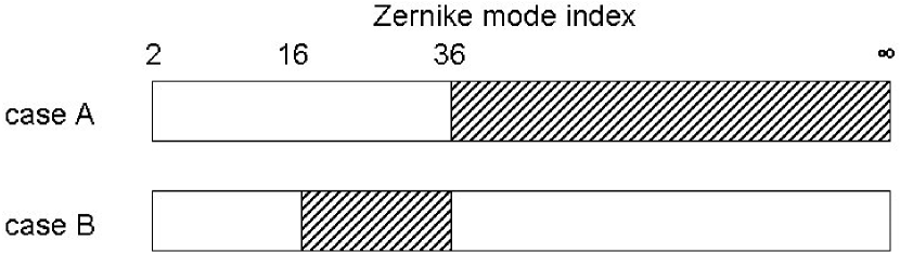
Figure 1: The hatched area of the bars indicate the spatial frequency range of the residuals, described by the index of the Zernike mode. Case A has been chosen because it mimics a case typical of a low-order AO system. Numbers of case B (residuals is the range $Z_{17-36}$) are chosen to provide the same wavefront flatness (same phase variance) as in case A. The two PSF will have the same phase variance, same SR, and same FWHM.

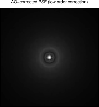
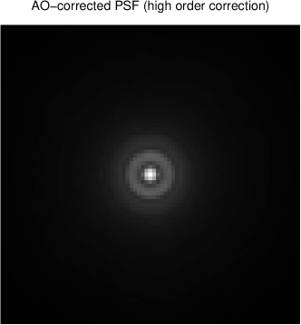
Figure 2: AO-corrected PSFs in the case of low order correction (perfect correction of ZPs up to $j_{max}=36$, left) and high order correction (perfect correction of ZPs 2 to 16 and 37 to $\infty$, right). 8 meter diameter telescope, seeing of $0.81~{}arcsec$ at $\lambda=0.5~{}\mu m$, H band ($\lambda=1.65~{}\mu m$). The simulated field of view is equal to $1.70\times 1.70~{}arcsec^{2}$.

For our illustration, we performed some Monte-Carlo numerical simulations of an AO corrected PSF, where the wavefront (from a fully developped Kolmogorov spectrum) is corrected by zeroing some coefficients of its expansion into Zernike polynomials (Noll, 1976). As we just study the influence of the compensation order, here we focus only on the spatial aspect of the correction, ignoring errors due to time delay, anisoplanatism or noise. The conditions of the simulation are a 8-meter telescope (VLT case), a seeing of $0.81~{}arcsec$ at $0.5~{}\mu m$ (median seeing of VLT site, Martin et al. (2000)), leading to a $r_{0}$ equal to $52~{}cm$ at the imaging wavelength of $1.65~{}\mu m$ (H band). We compared two clear-cut cases of correction, similar since they both lead to the same amount of residual phase variance $\sigma^{2}_{res}=0.0132(D/r_{0})^{5/3}~{}rad^{2}$, but different because the compensation concerns different domains of spatial frequencies, as illustrated in figure 1:

• for the case A, we mimic a typical low-order AO system, and we compensate for the polynomials $Z_{2}$ to $Z_{36}$. Phase residuals are high-order perturbations $Z_{>37}$.

• for the case B, we consider the phase residuals are now low-order perturbations in the range $Z_{17-36}$. Those last numbers are chosen so that the spatial frequency contents of the phase does not overlap with case A, but has exactly the same variance.

Figure 3: Radial profiles (left) and ensquared energy profiles (right) of the AO-corrected PSFs. The solid line corresponds to low order correction, the dashed line to high order correction.

The AO corrected PSFs in H band are shown on the figure 2, whereas figure 3 shows the radial (left) and ensquared energy profiles (right). Those figures aim to demonstrate how different the shapes of the PSFs can be, although they simultaneously exhibit identical residual phase variances, identical central intensities (predictable from the phase variance: both Strehl ratios are close to 30%), and identical FWHMs: the shapes of the coherent cores are identical, only the energy distribution of the halo is different, because it is strongly determined by the spatial contents of the phase residuals.

In terms of astrophysical implications, a PSF such as in case B (low-order residuals, right of figure 2) would be catastrophic for exoplanet detection, where the intensity in the first rings has to be minimised because of contrast issues. On the opposite, such a PSF is interesting for 3D spectroscopy as the ensquared energy is increased: this is particularly noticeable on the right of the figure 3.

One has therefore to keep in mind that for a fixed amount of phase variance removed, the ensquared energy will strongly be enhanced in the case of a high order compensation, which is particularly effective at reducing the halo compared to low-order modes correction. The conclusion is that the common rule of thumb, according to which the phase variance error budget should be balanced between undermodeling error and other sources, becomes obsolete when it is a matter of designing an AO system for spectroscopy. Despite the moderate resolution ($\approx 0.25~{}arcsec$) required, a rather large number of actuators is required to bring the light from the further parts of the halo into the inner parts, so as to increase the spectroscopic SNR, and only a high-order modes compensation can allow us to achieve this.

However, compensating for high order modes is not going without some difficulties from the AO point of view, the major limitation being anisoplanatism: high order modes unfortunately decorrelate faster with the separation angle (Chassat, 1989; Roddier et al., 1993). Unfortunately, the usual observing conditions of distant galaxies are at high galactic latitudes, where natural guide stars become scarce and are unlikely to lie within the isoplanatic patch $\theta_{0}$. This requires to work most of the time with large separation angles, that precisely forbid the compensation of high-order modes. This drawback makes classical AO unappropriate for the statistical studies of distant galaxies.

In the section 4 we will describe a new approach of adaptive optics, which solves anisoplanatism problems, which allows to use natural guide stars at distances greater than $\theta_{0}$, and which is still efficient to correct high order modes.

Before this, we want to be able to establish requirements about the ensquared energy needed for a proper statistical study on high redshift galaxies, in order to derive later some specifications for the AO system we propose.

3.3 Case study: 3D spectroscopy of UGC 6778 observed at high redshift

Thanks to numerical simulations, we show in the following subsections some quantitative results about the gain in spectroscopic SNR that can be achieved when AO and 3D spectroscopy are used together. We would like to emphasize here that we do not attempt to perform a complete simulation of a 3D spectrograph feeded by an AO system, because of the lack of 3D spectroscopic data currently available in the litterature for high redshift galaxies, and especially in the near-infrared wavelength range, where the $H\alpha$ emission line is observed for redshifts $z\geq 0.5$. We therefore do very simple assumptions about the instrument as well as the observed objects, in order to compute first estimates about the SNR achieved thanks to AO correction. Such results can be used to derive very preliminary required ensquared energy values, that can then be translated into instrumental requirements for the AO system. A $\Lambda CDM$ cosmology with $H_{0}=70$ km/s/Mpc, $\Omega_{m}=0.3$ and $\Omega_{\Lambda}=0.7$ is assumed in the rest of this paper.

UGC	Typea	$V_{VIR}^{\mathrm{b}}$	Db	$M_{B}^{\mathrm{a}}$	$R_{D}^{\mathrm{c}}$	$\mu_{D}^{\mathrm{c}}$	$i^{\mathrm{a}}$	PAa	$V_{max}^{\mathrm{a}}$
ID		(km s-1)	(Mpc)	(mag)	(kpc)	V/arcsec2	(∘)	(∘)	(km s-1)
3893	SBc	1193	17.04	-20.6	1.84	20.17	30	165	305

• from Garrido et al. (2002)

• from LEDA (http://www-obs.univ-lyon1.fr/hypercat/)

• from Baggett et al. (1998)

Table 1: Photometric and dynamic characteristics of UGC 6778. From left to right: the identifier of the galaxy, its morphological type, the recession velocity corrected from the local’s group infall toward Virgo $V_{VIR}$, the distance $D$ in Mpc, the absolute magnitude in B band $M_{B}$, the exponential disk scale lenght $R_{D}$, the disk surface brightness $\mu_{D}$, the inclination $i$ and the position angle $PA$, and the maximum velocity observed on the edge of the disk

We used for this study the $H\alpha$ image of the UGC 6778 galaxy provided by members of the GHASP survey (Garrido et al., 2002, 2003; Garrido et al., 2004; Garrido et al., 2005), with a spatial sampling $s_{0}=0.960~{}arcsec/pixel$. The table 1 lists the photometric and dynamic properties of this galaxy. These data were then used to simulate two science cases, where we assumed that the galaxy would be respectively located at $z=0.9$ or $z=1.5$, and that a microlens+fibers integral field spectrograph similar to GIRAFFE would be used to perform 3D spectroscopy on this galaxy.

The first steps required to perform these simulations are the following:

1. Use of the original $H\alpha$ image to simulate the distant galaxy image, taking into account the decrease of the apparent diameter due to redshift as well as the change of spatial sampling (see Giavalisco et al. 1996 for more information). We assumed a spatial sampling in the simulated galaxy image equal to half of the telescope’s diffraction limit (Nyquist sampling), i.e. $\lambda/2D$.

2. Computation of the apparent magnitude $m$ in the observing band (J or H) from nearby galaxy’s absolute magnitude $M$, using distance modulus, and taking into account the morphological K-correction $K(z)$ due to redshift into the distance modulus equation: $m-M=5\log(D_{L}/10)+K(z)$, where $D_{L}$ is the luminosity distance. We used values from Mannucci et al. (2001) for the K-correction. The flux in the continuum $f_{cont}$ (in $ergs~{}s^{-1}cm^{-2}\AA^{-1}$) can then be computed from the apparent magnitude $m$.

3. Computation of the total flux (in $ergs~{}s^{-1}cm^{-2}$) of the galaxy into the redshifted $H\alpha$ line, and normalisation of the simulated $H\alpha$ image.

4. Simulation of the distant galaxy continuum image assuming pure Freeman exponential profile, taking into account the disk scale length $R_{D}$ and the angular distance $D_{A}$. The flux normalisation is done using $f_{cont}$.

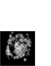
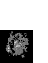
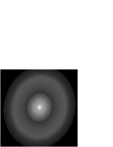
Original $H\alpha$ image	Simulated $H\alpha$ image	Continuum map
$z\approx 0.0$, $\lambda=0.656~{}\mu m$	$z=0.9$, $\lambda=1.250~{}\mu m$
$2.62\times 2.62~{}arcmin^{2}$	$1.80\times 1.80~{}arcsec^{2}$
$s_{0}=0.96~{}arcsec$	$s_{z}=0.016~{}arcsec$

Figure 4: Original $H\alpha$ image (left), simulated $H\alpha$ (middle) and continuum map (right) of the UGC 6778 galaxy as if it was observed at $z=0.9$ (in J band), with the same physical size than today. The simulated field is $1.80\times 1.80~{}arcsec^{2}$.

The figure 4 shows therefore the original $H\alpha$ image coming from the GHASP survey ($z\approx~{}0.0$, pixel size $s_{0}=0.96~{}arcsec$), as well as the simulated $H\alpha$ and continuum map corresponding to the first science case ($z=0.9$, pixel size $s_{z}=0.016~{}arcsec$).

We are going now to focus on the two $HII$ regions on the bottom left of the $H\alpha$ image. Garrido et al. (2002) have indeed shown that they have very similar velocities ($\approx 890$ km/s). We therefore do the assumption (sufficient for the rest of this study) that the integral field spectrograph we use has a sufficient spectral resolution $R$ so that the flux sampled around the wavelength $\lambda_{0}(1+v/c)$ (where $\lambda_{0}$ is the observing wavelength, i.e. 1.25 or 1.65 $\mu m$) is the flux only emitted in the $H\alpha$ line by these two regions, $v$ being their average velocity. We therefore isolated these two regions in the simulated images we created.

However the simulated $H\alpha$ and continuum images suppose infinite spatial resolution, and do not take into account atmospheric seeing or AO partial correction effects.

We therefore convolved those images with different point spread functions (PSF) corresponding to all the possible orders of AO correction, from 0 to 120 Zernike, at $1.25~{}\mu m$ and $1.65~{}\mu m$. The principle of the simulation is the same than in section 3.2, and we assumed the same conditions (8m telescope, seeing of $0.81~{}arcsec$ at $\lambda=0.5\mu m$, no anisoplanatism, noise or temporal error). As a consequence of this AO compensation, a better contrast in the images as well as a better ensquared energy is observed, as already explained in section 3.1. The result of the AO impact is illustrated, for a few cases, on figure 5.

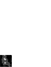
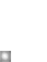
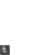
Figure 5: Illustration of the effect of adaptive optics compensation on the images. The simulated images cover a field of $0.50\times 0.50~{}arcsec^{2}$ ($4\times 4$ microlenses of $0.125\times 0.125~{}arcsec^{2}$). A analysis has been done, that covers compensation orders from 0 to 120 Zernike modes. A few cases have been picked up and are presented here for illustration purpose. From left to right: diffraction-limited image, seeing-limited image, AO-corrected image for 46 and 100 ZPs.

Those images could then be used to compute the flux entering into the microlens sampling each $HII$ region, and then compute the final number of electrons on each pixel of the detector located at the output of the spectrograph, requiring therefore to know the spectral profile of the line. We assumed a gaussian line profile for the line, being the consequence of some internal velocity dispersion $\sigma_{V}$ in those $HII$ regions, as well as the finite spectral resolution $R$ of the spectrograph. As a result, the line profile on the spectrograph detector has a gaussian shape, with a standard deviation $\sigma_{tot}=\sqrt{\sigma_{V,\lambda}^{2}+\sigma_{S}^{2}}$, $\sigma_{V,\lambda}=\lambda_{0}\times\sigma_{V}/c$ being the standard dispersion in wavelength due to the internal velocity dispersion of the $HII$ regions, and $\sigma_{S}=\lambda_{0}/2.354R$ being the standard deviation due to the spectral resolution, with $\lambda_{0}$ being the observing wavelength and $c$ the light celerity. Therefore, if we call $F_{ML}$ the total flux in HII region sampled by the spectrograph’s microlens, the line’s profile $f(\lambda)$ as a function of wavelength will be written:

$$f(\lambda)=\frac{F_{ML}}{\sigma_{tot}\sqrt{2\pi}}\exp{-\frac{\left(\lambda-\lambda_{0}\right)^{2}}{2\sigma_{tot}^{2}}}$$ (1)

This line profile is then going to spread over two directions on the spectrograph’s detector: the horizontal direction will correspond to the spectral information, and the perpendicular direction will correspond to the spatial information. This allows us to compute the number of electrons due to the $H\alpha$ line per pixel on the spectrograph detector, and then the spectroscopic SNR. If $\Delta\lambda$ is the spectral sampling of the detector, $S_{tot}$ the telescope area, $t_{exp}$ the exposure time, and $T_{tot}$ the total transmission of the system (which takes into account the detector efficiency), the number of electrons $N_{H\alpha}$ coming from the redshifted $H\alpha$ line on the pixel sampling the line at the $\lambda_{0}$ wavelength is then equal to:

$$N_{H\alpha}=2\int_{0}^{\Delta\lambda/2}f(\lambda)d\lambda\times S_{tot}\times t_{exp}\times T_{tot}\times\lambda_{0}/hc$$ (2)

where $h$ and $c$ are respectively the Planck constant and the speed of light.

We then have the flux from the line going onto the detector pixel. However, as we are interested in computing the spectroscopic SNR, we therefore need to take into account all the sources of noise, which can be divided in three categories: the line and continuum photon noise, the background photon noise, and the detector noise. As both line and continuum signals have poissonnian statistics, therefore their associated photon noise has a variance equal to their respective value, i.e. $N_{S}$ and $N_{cont}$, where the number of electrons $N_{cont}$ due to the continuum is equal to:

$$N_{cont}=f_{cont}\times S_{tot}\times t_{exp}\times\Delta\lambda\times T_{tot}\times\lambda_{0}/hc$$ (3)

$f_{cont}$ being the flux from the continuum entering the microlens after convolution of the continuum image by the AO corrected PSF. Concerning the background noise, this latest is the sum of the sky background as well as the instrumental thermal background. Then, if we call $N_{B}$ the total number of electrons coming from the backgroud, as it has also Poisson statistics, its associated photon noise will then have a variance equal to $N_{B}$. At last, detector noises, i.e. dark current noise and readout noise, have to be considered.

Knowing all these values, we can then compute the SNR per spatial resolution element and per spectral pixel, which will be written:

$$SNR=\frac{N_{H\alpha}}{\sqrt{N_{H\alpha}+N_{cont}+N_{B}+N_{pix,spat}(N_{D}+N_{exp}\sigma_{R}^{2})}}$$ (4)

with:

• $N_{B}$ the number of electrons coming from the instrumental and sky background

• $N_{D}=DC\times T_{exp}$ the number of electrons dues to the dark current DC (in $e^{-}/s/pix$)

• $N_{exp}$ the number of elementary exposures

• $\sigma_{R}$ the readout noise (in $e^{-}/pix$)

• $N_{pix,spat}$ the number of pixels on which the flux is spread in the spatial direction on the detector
  

The equation 4 therefore gives the expression SNR on the measured quantities. However, the figure 5 shows that as the AO correction improves, the image contrast becomes better, with an increase of the effective light coming from the $HII$ region. As a result, the flux going into the microlens sampling each HII region is therefore the sum of two terms: the effective flux emitted by the $HII$ region, and a pollution term coming from adjacent regions, which is going to degrade the spectrum of the area sampled by the microlens, provided as an output of the 3D spectrograph. This has leaded us to define another signal-to-noise ratio, which we will call Effective signal-to-noise ratio (ESNR), and which gives a measure of the effective gain provided by the coupling of AO with 3D spectroscopy. Its expression is:

$$ESNR=\frac{N_{H\alpha,eff}}{\sqrt{N_{H\alpha}+N_{cont}+N_{F}+N_{pix,spat}(N_{D}+N_{exp}\sigma_{L}^{2})}}$$ (5)

Figure 6: Explanation of the effective flux notion. The first image on the left shows the original image, with the two $HII$ regions and the superposed microlens (in dashed line). The second image shows only the area sampled by the microlens. The third and fourth show this latter convolved by the uncorrected PSF (third) and by an AO-corrected PSF (fourth image, correction of 60 ZPs). The effective flux from the $H\alpha$ line is then equal to the flux of the region after convolution by the PSF going into the microlens.

where $N_{H\alpha,eff}$ is the number of electrons due to the effective $H\alpha$ flux emitted by the area sampled by the microlens after convolution by the AO corrected PSF, with no contribution from the adjacent areas around the microlens. This notion of effective flux is explained on the figure 6.

One will notice that denominators in the equations 4 and 5 are the same, and therefore that the ESNR is a lower bound of the SNR. This is explained by the fact that in the case of the ESNR, all the noise sources must appear in the denominator. Concerning the line, this latter is perturbed by a noise, which is the sum of two terms: the photon noise of the effective flux, and a pollution term due to all the light coming from the area around the microlens and entering the microlens because of the convolution. As both quantities have poissonnian statistics, and as the convolution operator is distributive, the sum of these two terms is equal to the photon noise of the measured light entering the microlens.

We would however like to emphasize here that the ESNR defined at the equation 5 and the classical SNR definition shown in equation 4 cannot be directly compared, in particular when the ensquared energy changes. As it is shown in figure 6, the ESNR numerator is the flux coming only from the region sampled by the microlens after convolution by the AO corrected PSF, whereas the SNR numerator is the flux not only coming the microlens, but also the flux from adjacent areas and polluting the microlens because of the convolution. As different images are convolved for ESNR and SNR computations, there is no direct relation (i.e. multiplication) between these numbers. Moreover, as explained in the section 3.1, an increase of the ensquared energy is due to a better compensation order provided by the AO system. Thus different ensquared energy values correspond to different AO corrected PSFs, and the results of the convolution of the same high-resolution galaxy image by these different PSFs also cannot directly be comparable.

Once these two different quantities (SNR and ESNR) defined, we performed some numerical simulations in order to quantify the gain in ESNR provided by the combination of AO with 3D spectroscopy. The results of these simulations are shown in the next section.

3.4 Results

Thanks to simulations, we are now able to show some preliminary results about the improvement in ESNR thanks to AO. Two science cases, corresponding to the observation of UGC 6778 at two different redshifts, are considered in the two next subsections.

For the first one, we assumed that the observed galaxy would be located at $z=0.9$. In that case, the $H\alpha$ emission line is redshifted at a wavelength of $1.25~{}\mu m$, corresponding to the central wavelength of J band. Moreover we assumed that the galaxy had the same properties than the distant large spirals observed in the CFRS (Lilly et al., 1998; Zheng et al., 2004). In particular the physical size of the simulated galaxy is the same than the one observed in the local universe. As there are no direct measurements of $H\alpha$ fluxes available in the litterature for CFRS galaxies at these redshift, we therefore computed the $H\alpha$ luminosity from $[OII]3727$ fluxes (Hammer et al., 1997), in order to normalise the simulated $H\alpha$ image.

For the second one, we assumed that the observed galaxy would be located at $z=1.5$. In that case, the $H\alpha$ emission line is redshifted at a wavelength of $1.65~{}\mu m$, corresponding to the central wavelength of H band. Moreover we assumed that the galaxy had $H\alpha$ fluxes similar to the ones observed on the population of ”‘BM galaxies”’ introduced by Steidel et al. (2004). The apparent size of the galaxy was then chosen to cover a field of $1~{}arcsec^{2}$, consistent with apparent sizes observed on distant galaxies at these redshifts in deep surveys (Bouwens et al., 2004).

We focus now on the two $HII$ regions we used to compute the SNR and ESNR. Together they contribute at $10\%$ of the total $H\alpha$ flux in the simulated $H\alpha$ image. We also assumed that they had an internal velocity dispersion with $FWHM_{V}=30~{}\mathrm{km.s^{-1}}$ (eg $\sigma_{V}\approx 13~{}\mathrm{km.s^{-1}}$), leading as explained previously to a dispersion in wavelength on the spectrograph’s detector equal to $\sigma_{\lambda,V}=\lambda_{0}\times\sigma_{V}/c$, $\lambda_{0}$ being equal to 1.25 or 1.65 $\mu m$. The spectral resolution was then fixed to $R=10000$, allowing to resolve the velocity dispersions of the $HII$ regions. This then allowed us to define two cases of spectral sampling, corresponding to the horizontal direction on the spectrograph’s detector: $\Delta\lambda=0.3\AA/pix$ (for J band) or $\Delta\lambda=0.6\AA/pix$ (for H band). Such spectral samplings allow us to sample the spectral resolution with more than two pixels, thus providing a better sampling than Nyquist sampling, and then do a precise estimation of the barycenter of the $H\alpha$ emission line in order to recover the galaxy’s velocity field. For the vertical direction on the spectrograph’s detector, corresponding to the spatial information, we considered a number of pixels $N_{pix,spat}=3$, similar to the number of pixels used on the GIRAFFE spectrograph’s detector. Such a number of pixels, here again better than Nyquist sampling, is quite convenient to resolve spectrum deblending problems on the spectrograph’s detector.

For the sky background, we assumed that the spectrograph is observing between atmospheric OH lines, so the sky noise is equal to the sky continuum. Cuby (2000) has measured the sky continuum at the Cerro Paranal observatory, and found respective values of 1200 $ph/s/m^{2}/\mu m/arcsec^{2}$ at a wavelength of 1.25 $\mu m$, and 2300 $ph/s/m^{2}/\mu m/arcsec^{2}$ at a wavelength of 1.65 $\mu m$. We used the characteristics of the VLT’s ISAAC spectrograph to simulate the instrument: the instrumental background was assimilated to a blackbody of temperature $T=273K$ and an emissivity equal to $25\%$, a total transmission (atmosphere+telescope+instrument+detector) of $13\%$ at $1.25~{}\mu m$ (central wavelength of J band) and $19\%$ at $1.65\mu m$ (central wavelength of H band) was assumed, and the detector had a dark current $DC=30e-/h/pix$ and a readout noise $RON=10~{}e-/pix$.

3.4.1 First science case: 3D spectroscopy of UGC 6778 at $z=0.9$

Here we give the results of simulations of the 3D spectroscopy of UGC 6778 as if it was observed at $z=0.9$. We assumed that the galaxy had the same physical size as it has now. However the flux in the $H\alpha$ line is consistent with the one observed of distant galaxies. Such physical conditions correspond to the ones observed on large spirals in the distant universe (Lilly et al., 1998; Zheng et al., 2004).

The original $H\alpha$ image covers a field of $2.62\times 2.62~{}arcmin^{2}$, and the galaxy has a distance $D=17.04$ Mpc, which leads to a physical field of $d_{1}\times d_{1}~{}kpc^{2}$, with $d_{1}=13.40~{}kpc$. Now, if we assume that the same galaxy has a redshift $z$, we can then compute its luminosity-distance $D_{L}$ and its angular distance $D_{A}$, and we found that the observed field has therefore an apparent size equal to $\theta_{z}\times\theta_{z}~{}arcsec^{2}$, with $\theta_{z}=d_{1}/D_{A}=1.80~{}arcsec$. Moreover, the spatial sampling is not the same as we simulate the galaxy as if it was observed by the VLT (8 meter diameter telescope) at its diffraction limit, meaning the pixel sampling $s_{z}$ is equal to Nyquist sampling ($\lambda/2D$), leading to a pixel size $s_{z}=0.016~{}arcsec$. Therefore the number of pixels in the original and simulated images are not the same: as shown in figure 4, the original image has $164\times 164$ pixels, whereas the simulated image has $111\times 111$ pixels.

This simulated image must be then normalized so that its flux is equal to the flux in the $H\alpha$ line. As explained before, there are not direct measurements of $H\alpha$ fluxes on the CFRS galaxies, therefore we used $[OII]3727$ luminosities to compute $H\alpha$ fluxes. Hammer et al. (1997) found that the average rest-frame equivalent width of the $[OII]3727$ line in CFRS galaxies located at $z=0.9$ was equal to $EW([OII]3727)=40\AA$. Moreover, Kennicutt (1992) found that there is a relation between the equivalent width in the $[OII]3727$ and $H\alpha$ line, in the form $EW(H\alpha)=2.5\times EW([OII]3727)$. We therefore assumed that the $H\alpha$ line had a rest frame equivalent width $EW(H\alpha)=100\AA$.

Once $EW(H\alpha)$ is known, the flux in the continuum $f_{cont}$ must be computed to know the flux $f_{H\alpha}$ in the $H\alpha$ line, as both are linked to the relation: $f_{H\alpha}=f_{cont}\times EW(H\alpha)\times(1+z)$. $f_{cont}$ is directly linked to the apparent magnitude of the galaxy. We see on the table 1 that UGC 6778 has an absolute magnitude in B band $M_{B}=-20.6$. However, as the $H\alpha$ line is redshifted in J band, we are interested by the galaxy’s absolute magnitude in J band. For a SBc galaxy like UGC 6778, Mannucci et al. (2001) give the following colours: $(B-V)=0.70$, $(V-K)=3.03$, $(J-H)=0.66$ et $(H-K)=0.25$. We then find an absolute rest-frame magnitude $M_{J}=-23.42$. Mannucci et al. (2001) give also the following K-correction for a Sc galaxy: $K(z=0.9)=0.155$. The redshift $z$ can then be used to compute the luminosity distance $D_{L}$ and the distance modulus. We therefore find an apparent magnitude $J=20.41$, corresponding to a flux in the continuum $f_{cont}=8.09\times 10^{-19}~{}ergs/cm^{2}/s/\AA$, leading to a $H\alpha$ flux of $4.17\times 10^{-17}~{}erg/s/cm^{2}$. This flux was then used to normalise the simulated $H\alpha$ image.

As explained before, the continuum emission has also to be taken into account. This latter is not equally spread over the galaxy, as the intensity of disk in spiral galaxies follows a decreasing exponential law (Freeman, 1970), in the form $I(r)\propto\exp^{-r/R_{d}}$, $R_{d}$ being the disk scale length, whose value for UGC 6778 is given in table 1. It is therefore possible to compute $R_{D,z}$, the angular size of of the disk scale length when the galaxy is observed at a redshift $z$, by the relation $R_{D,z}=R_{D}/D_{A}$, $D_{A}$ being the angular diameter distance, and we found a value of $R_{D,z}=0.25~{}arcsec$. This value, as well as the position angle $PA$ of the galaxy and the inclination $i$ (which are given in the table 1), were used to compute the continuum map of the galaxy. This latter was then normalised so that its total flux was equal to $f_{cont}$. The simulated $H\alpha$ image as well as the continuum map are shown on the figure 4.

Figure 7: Measured spectroscopic SNR (top) and effective spectroscopic SNR (ESNR, bottom) on the $H\alpha$ line for a microlens of $0.125~{}arcsec$ as a function of the ensquared energy in a $0.25\times 0.25~{}arcsec^{2}$ square aperture. The considered galaxy is located at $z=0.9$ (observation in J band) and has the same characteristic of distant large spirals. Each curve corresponds to the average of the SNR of each microlens sampling the HII regions, microlens, with exposure times going from 1 hour to 8 hours. The dashed line corresponds to $SNR=3$.

Once those two images created, it is possible to compute the measured spectroscopic and effective SNR per spectral pixel. However, as our goal is to show the gain given by the combination of AO with 3D spectroscopy, we convolved these latter images by simulated AO corrected PSFs, with a degree of correction going from 0 ZPs (seeing-limited PSF) to 120 ZPs, leading to an increase of the ensquared energy as the number of corrected modes increases. We also considered exposure times between 1 and 8 hours, with individual exposure times of 1 hour. The figure 7 shows the evolution of these SNRs as a function of the ensquared energy into a $0.25\times 0.25~{}arcsec^{2}$ square aperture. More precisely, if we look at the evolution of the ESNR which in fine says the real improvment provided by AO correction, we see that a minimum ensquared energy of $26\%$ allows to reach an ESNR of 3 after an exposure time of 8 hours. However, a slightly increase to an ensquared energy of $30\%$ allows to reach the same ESNR value, but only after 3 hours of exposure time.

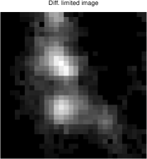
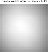
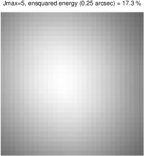
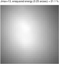
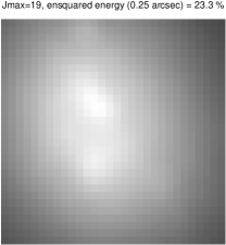
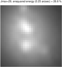
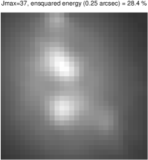
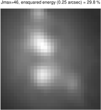
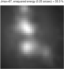
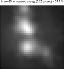
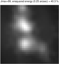
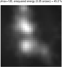
Figure 8: Images of the HII regions convolved with the AO corrected PSF, for different levels of AO correction in J band. The title of each image shows the number of corrected modes and the corresponding ensquared energy into a $0.25\times 0.25~{}arcsec^{2}$. The field of view is equal to $0.50\times 0.50~{}arcsec^{2}$ ($4\times 4$ 0.125 arcsec microlenses).

As it was shown previously, the AO correction not only increases the ensquared energy into the spatial resolution element, but it also increases the sharpness of the AO corrected PSF, therefore providing a better image contrast. This is indeed shown on the figure 8, where it can be seen that the two HII regions start to be well separated after the perfect correction of the first 46 Zernike Polynomials. This level of AO correction corresponds to an ensquared energy equal to $28\%$ into a $0.25\times 0.25~{}arcsec^{2}$ square aperture.

This study has therefore shown that the combination of 3D spectroscopy with AO is definitely effective in terms of angular resolution and SNR improvement. This means that the 3D spectroscopy of $z\approx 1$ galaxies with an angular resolution of $0.25~{}arcsec$ (definitely better than atmospheric seeing) should be achievable on a 8 meter telescope located on the ground such as the ESO VLT. This requires the AO correction to provide a minimum ensquared energy of $28\%$ in a $0.25\times 0.25~{}arcsec^{2}$ square aperture. In that case, a spectral resolution $R=10000$, allowing to resolve velocity dispersions with $FWHM_{V}\geq 30~{}km/s$, can be used, as an effective spectroscopic SNR of 3 can be reached after an exposure time of only three hours.

3.4.2 Second science case: 3D spectroscopy of UGC 6778 at $z=1.5$

We give here the results of simulations of the 3D spectroscopy of UGC 6778 as if it was observed at $z=1.5$. We assumed here that the galaxy covers an apparent surface of $1~{}arcsec^{2}$, which is consistent with apparent sizes measured on deep surveys. This apparent surface was then used to simulate the apparent $H\alpha$ and continuum images. We are then going to focus on the continuum and $H\alpha$ flux normalisation.

We used the data from Erb et al. (2003) and Steidel et al. (2004), who observed with the LRIS spectrograph on the Keck telescope a sample of BM/BX galaxies located between $z=1.4$ and $z=2.5$. Erb et al. (2003) found on their sample ($\left\langle z\right\rangle=2.28$) an average apparent magnitude $\left\langle R\right\rangle=24.37$, and an average apparent $H\alpha$ flux $f(H\alpha)=4.6\times 10^{-17}~{}ergs~{}s^{-1}~{}cm^{-2}$. One will notice that the apparent $H\alpha$ flux is comparable to the one computed in the previous science case $(z=0.9)$ where we simulated the observation of a distant large spiral galaxy belonging to the CFRS. In fact the two science cases have been chosen using previous well-known studies of distant galaxies. At $z=0.9$, the CFRS has studied average $L^{*}$ galaxies, while at $z=1.5$, Erb et al. (2003) have focused on a sample of specifically $H\alpha$ luminous galaxies.

Moreover Steidel et al. (2004) found that galaxies with a redshift $\left\langle z\right\rangle=2.23\pm 0.31$ had an average color $\left\langle R-K\right\rangle=3.25\pm 0.53$. We therefore found that those galaxies had an apparent magnitude $\left\langle K=21.12\right\rangle$. It is therefore possible to compute their K absolute magnitude $M_{K}$ using again the distance modulus, assuming a k-correction $K(z)=-0.57$ at $z=2.3$ (extrapolation to $z=2.3$ of the k-correction in K band given by Mannucci et al. for a Sc galaxy), leading to $M_{K}=-24.38$. Moreover, as Sc galaxies have a color $(H-K)=0.25$ (Mannucci et al., 2001), we found that such a galaxy has a rest-frame H absolute magnitude equal to $M_{H}=-24.13$. Assuming a k-correction $K(z)=0.078$ at $z=1.5$ for a Sc galaxy observed in H band (Mannucci et al., 2001), we therefore found an apparent magnitude $H=20.99$ for the case where such galaxies would be located at $z=1.5$, corresponding to a flux in the continuum $f_{cont}=1.67\times 10^{-19}~{}erg/s/cm^{2}/\AA$.

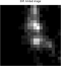
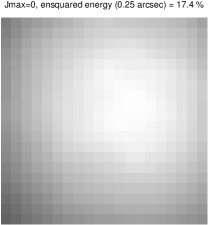
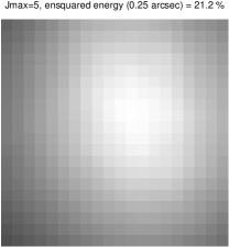
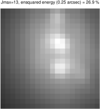
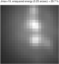
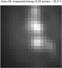
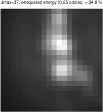
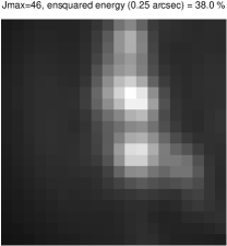
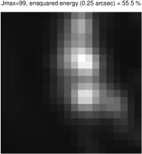
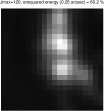
Figure 9: Images of the HII regions convolved with the AO corrected PSF, for different levels of AO correction in H band. The title of each image shows the number of corrected modes and the corresponding ensquared energy into a $0.25\times 0.25~{}arcsec^{2}$ square aperture. The field of view is equal to $0.50\times 0.50~{}arcsec^{2}$ ($4\times 4$ 0.125 arcsec microlenses).

Figure 10: Measured spectroscopic SNR (top) and effective spectroscopic SNR (ESNR, bottom) on the $H\alpha$ line for a microlens of $0.125~{}arcsec$ as a function of the ensquared energy in a $0.25\times 0.25~{}arcsec^{2}$ square aperture. The considered galaxy is located at $z=1.5$ (observation in H band) and covers an apparent field of $1~{}arcsec^{2}$. Each curve corresponds to the average of the SNR of each microlens sampling the HII regions, with exposure times going from 3 hour to 24 hours. The dashed line corresponds to $SNR=3$.

These flux values were used to normalise the simulated images of the distant galaxy. Then we did the same computations as previously explained, in order to compute the measured spectroscopic and effective SNR per spectral pixel on the spectrograph’s detector, and especially show the improvements provided by AO correction. This time we considered exposure times from 3 to 24 hours. The result of these simulations is shown on figure 10, where we can see that an effective SNR of 3 can be reached after a minimum exposure time of 9 hours, requiring an ensquared energy after AO correction equal to $60\%$ into a $0.25\times 0.25~{}arcsec^{2}$ square aperture. The same ESNR value can be reached with an ensquared energy after AO correction equal to $40\%$, requiring then an exposure time of 18 hours, or also with an ensquared energy after AO correction equal to $33\%$, requiring then an exposure time of 24 hours. However, in the previous section we saw that a minimum ensquared energy must also be reached so that the two HII regions can be separated. This is explained in the figure 9, where we can see that the two HII regions start to be separated for an ensquared energy after AO correction better than $30\%$.

This study has therefore shown that the combination of 3D spectroscopy with AO should allow also to perform the 3D spectroscopy of galaxies located at $z=1.5$, also with an angular resolution of $0.25~{}arcsec$ (definitely better than atmospheric seeing) and with a spectral resolution $R=10000$, allowing to resolve velocity dispersions $FWHM_{V}\geq 30~{}km/s$, as well as reaching effective spectroscopic SNR of 3. This can be achieved with a minimum ensquared energy after AO correction of $35\%$ and an exposure time of 24 hours, knowing that the same ESNR value can be reached with an ensquared energy of $40\%$ and a shorter exposure time (18 hours).

3.5 Conclusion

We studied in this section the improvement provided by the combination of 3D spectroscopy with Adaptive Optics (AO). Firstly we have shown that thanks to AO, it is possible to reach angular resolution better than seeing, but also to increase the spectroscopic signal-to-noise ratio (SNR), allowing to perform 3D spectroscopy of distant galaxies, thus studying their kinematics. We have then performed some simulations allowing to give some preliminary performance of an integral field spectrograph providing an angular resolution of $0.25~{}arcsec$ and a spectral resolution $R=10000$, and which would observe distant galaxies located at $z=0.9$ and $z=1.5$. In that case, the $H\alpha$ emission line is redshifted in the central wavelengths of J and H bands (respectively $1.25~{}\mu m$ and $1.65~{}\mu m$). To quantify the performance of such an instrument, we have defined a new criterium called ”‘Effective signal to noise ratio”’ (ESNR). We also assumed for those simulations galaxies with properties consistent with the ones observed in distant surveys. We have therefore shown that an ESNR of 3 can be reached for a galaxy located at $z=0.9$, requiring a minimum ensquared energy into a $0.25\times 0.25~{}arcsec^{2}$ after AO correction equal to $30\%$ and an exposure time of 3 hours. The same ESNR value can be reached for a galaxy located at $z=1.5$, requiring then a minimum ensquared energy after AO correction of $35\%$ and an exposure time of 24 hours, however a slight increase of the ensquared energy to $40\%$ should allow to reach the same ESNR value after an exposure time equal to 18 hours.

A study of the AO corrected PSF has shown that high order modes need to be corrected to improve the ensquared energy. This has been confirmed by our simulations of the 3D spectroscopy of distant galaxies, where we found that at least 46 Zernike polynomials need to be corrected to reach an ensquared energy of $30\%$ in J band and $40\%$ in H band (such results are not definitive, as we used the dynamical properties of one galaxy observed in the local universe as well as those of a few distant galaxies, but they can be used as a first basis, the data required to perform such studies being still rare in the community). Such a number of modes corresponds in fact to the minimum order of modes to correct, as we assumed a perfect AO system in our study. In a real AO system, other sources of error like time delay, measurement noise and anisoplanatism are going to degrade the performance of AO, meaning that a larger number of modes will be required to reach the same ensquared energy values and image quality. We must especially insist on the fact that anisoplanatism is going to become the most important limitation in the case of a real instrument using both AO and 3D spectroscopy. Indeed, as extragalactic studies require to work at high galactic latitudes, the probability of finding a suitable star to perform wavefront sensing is equal to a few percents, meaning that AO, at least in its classical form, cannot be used because of its very low sky coverage.

We are therefore going to describe in the next sections the principle and the performance of FALCON, a project of a multi-object 3D spectrograph with AO, which solves the sky coverage’s problem imposed by classical AO. FALCON uses the principle of Multi-Object Adaptive Optics (MOAO). Such a technique allows to widen the useful field of view of AO systems, thus to perform the simultaneous 3D spectroscopy of several distant galaxies in a very wide field of view, providing therefore a huge gain in terms of observing time efficiency.

4 The FALCON’s AO system: principle

4.1 Increase of the AO corrected FoV: MCAO and tomography

As stated in the introduction, Adaptive Optics, in its classical form where one guide star (GS) and one deformable mirror (DM) conjugated to the pupil are respectively used to measure and correct the turbulent wavefront, suffers from a very low sky coverage (less than $5\%$), even at galactic latitudes of $30^{\circ}$. The reason of this limitation is that the probability to find a suitable GS in the isoplanatic patch is generally very low, due to the distribution of the stars in our galaxy.

Such a limitation has leaded to the development of Multi-Conjugate Adaptive Optics (MCAO). In MCAO, several deformable mirrors conjugated to the turbulent layers are used to correct the phase in the turbulent volume. Indeed, this is the repartition of the turbulence in the altitude which is responsible for anisoplanatism, as the wavefronts coming from different directions do not cross the same volume of the atmosphere (especially for high turbulent layers), and therefore do not suffer from the same degradations. By correcting the phase in the turbulent volume, and especially in the strongest layers, it is possible to correct the wavefront for any direction, and to have an uniform compensation in a field of view larger than the isoplanatic patch.

Before correcting the phase with the different DMs, it is required to know the perturbation in each layer to apply to each DM the adequate commands. This can be achieved thanks to tomography (Ragazzoni et al., 1999, 2000; Tokovinin & Viard, 2001), where the light coming from several off-axis GSs far outside of the isoplanatic patch is used to probe the 3-dimensional phase perturbations in the atmosphere, generally by solving an inverse problem as in medical imaging. However, thanks to tomography, it is also possible to know the integrated phase perturbation in the pupil for any direction in the field of view. This means the field where GS can be found is widened, and this allows a higher sky coverage for AO (Tokovinin et al., 2001).

However, the potential extension of the field of view with MCAO encounters some technical limitations, in particular on the optical system. As an example, the ESO-MAD system for the VLT Marchetti et al. (2003) or the Gemini-South MCAO system Ellerbroek et al. (2003) will deliver a corrected field of view with a diameter of 2 arcmin, definitely smaller than the $10\times 10~{}arcmin^{2}$ field of view required for extragalactic studies. We are therefore going to show in the next paragraph a new approach for AO, where the goal is not to provide an uniform correction in a very wide field of view, but only for specific areas into it, i.e. the galaxies on which we want to perform 3D spectroscopy. This new approach is called Multi-Object Adaptive Optics (MOAO).

4.2 Multi-Object Adaptive Optics

First proposed by Hammer et al. (2002), Multi-Object Adaptive Optics (MOAO) is a new method of AO correction which has essentially been since this date the object of a few conference proceedings papers (Assémat et al., 2004; Dekany et al., 2004; Hammer et al., 2004). We summarise its principles in this section.

Let us recall here that our goal is to measure the internal kinematics of distant galaxies spread over the VLT Nasmyth field. In other words, this means that a high angular resolution is required only for the scientific targets. As a result, we propose in this section a totally new approach for AO: instead of correcting the whole $10\times 10~{}arcmin^{2}$ field (which anyway is impossible to do), we propose to correct locally only the regions of interest, $i.e.$ the integral field units positioned on the scientific targets, and we have therefore one AO system per integral field unit. As a result, if we suppose that we want to perform the simultaneous 3D spectroscopy of 20 galaxies, we arrive to the concept of an instrument using 20 multiple AO systems, spread in the VLT Nasmyth focal plane, and working in parallel independently of each other.

Although the complexity of such an instrument may appear insuperable at first sight, it can be greatly relaxed thanks to the tininess of the compensated field required for each independent galaxy. Indeed, as already demonstrated by the instrument GIRAFFE (Hammer et al., 1999), a field of view of only $3\times 2~{}arcsec^{2}$ is sufficient to measure the velocity fields of large spirals at $z\leq 1$, as well as galaxies with smaller apparent sizes observed at greater redshifts. This is one order of magnitude smaller than the isoplanatic patch in the near-infrared, so only one unique deformable mirror conjugated to the pupil is required to correct the whole galaxy.

Moreover, we propose a concept where the AO system is miniaturized. Each IFU, laying in the telescope focal plane, will include its proper micro deformable mirror -with a proper tiny pupil imaging optics. The wavefront sensors also lay a few centimeters apart, in the focal plane ; they are located on the guide stars surrounding the galaxy. Translated into length units in the VLT focal plane, an apparent size of $3\times 2~{}arcsec^{2}$ covers a physical size of $1.8\times 1.2~{}mm^{2}$, and a median distance of 1 arcmin between galaxy and guide stars translates into $\approx 35~{}mm$. Those numbers suggest the size of the system we propose: the adaptive IFU, and the WFSs have to be integrated into suitable optomechanical devices, which should not be too wide (typically less than $20~{}mm$) in order not to obstruct the focal plane and allow to use of the closest suitable guide stars for wavefront sensing. Such an integration of the subsystems, together with a separation of their functions (the DM and the WFS become separate, physically independent items), allow to move those devices into the VLT focal plane just as the positioner OzPoz does with the IFUs used on GIRAFFE (Hammer et al., 1999).

In addition to offer an obvious multiplex advantage, the proposed structure combined with a tomographic wavefront sensing approach allows us to overcome the sky coverage problem. Several guide stars, far out the isoplanatic patch, are used around each IFU to sense the wavefront. For a 8 meter diameter telescope, it has been shown (Fusco et al., 1999) that 3 WFSs are sufficient to reconstruct the phase in the pupil for any direction in a field of view of $\approx 2~{}arcmin$ diameter and for any turbulence profile; using more WFSs only brings a marginal improvement.

We chose to focus our study on natural guide stars. We believe that using Laser Guide Stars (LGS), although very attractive and apparently drastic solution at first sight, could be technically exponentially difficult to implement when dealing with an increasing number of beacons (minimum of 20 beacons here), while bringing its set of inherent problems such as cone effect, beacon elongation, superimposition of Rayleigh scattering and beacons, etc. Our approach was then to start the study on NGS, at the risk of doing the study again with LGS in the case where it would be demonstrated that NGS do not allow to fill the requirements.

We emphasize that the architecture described above corresponds to an open-loop system, since the WFS does not get any optical feedback from the deformable mirror of the adaptive IFU: this drastically differs from classical closed-loop AO systems. This is of course extremely challenging in terms of AO components. Firstly, the drifts, the linearity, the hysteresis and the calibration of the DM must be kept to a very low error level in order to be able to control it accurately enough in open-loop. Secondly the WFS must have a high dynamic range in order to provide reliable absolute open-loop measurements, together with a high sensitivity versus flux level. Such a WFS does not currently exist and needs to be developped, although some similar attempts have been done in the field of a posteriori speckle imaging (Lane et al., 2003). Thirdly, the miniaturisation of the components will undoubtly demand a large technical effort.

On the other hand, an architecture where the optical system is distributed all over the field has the considerable advantage to simplify the optics. In particular, the field selection functionnality becomes here a built-in function, when the amount of technical difficulties and the sharp specifications are often underestimated in classical systems. Not only this critical part does not exist any more, but the overall optical throuput of the instrument is boosted, as, at any moment, no dichroic plate is needed to split the light, and because the number of optical surfaces is reduced to its strict minimum. It is important to keep in mind that the efforts put in this instrument are undertook to gain not only in spatial resolution, but also in signal-to-noise ratio. On this latter particular point, the instrument optical throughput does matter even more than the AO performance, which, in return, will be increased when the WFS optical transmission is better.

In order to evaluate the system performance in terms of its dimensionning, we ran some numerical simulations. Their presentation and results are the scope of the following section. Those simulations assume that we have 3 natural guide stars per IFU, an a tomographic reconstructor. They are independent of any detailled system configuration, such as the miniaturisation of components or the error inherent to open-loop aspects. In this way, they could still apply whatever the technical solution. As an example, a system where the Nasmyth field would be optically sliced into sub-fields, themselves sent to independent closed-loop mono-mirror tomographic multi-analysis systems, would lead to the same results.

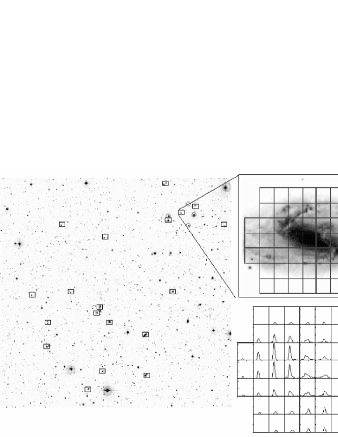
Figure 11: The Falcon concept combines MOAO and tomography: several IFUs (rectangles) are spread over the VLT focal plane. Each IFU is used to perform the 3D spectroscopy of one galaxy. Three miniaturised WFSs (circles) measure the wavefront coming from 3 off-axis NGS located around the galaxy. Their combined signals are used, through a tomographic reconstructor, to command the miniaturised DM into the IFU and correct the wavefront. It is therefore possible to recover the velocity field of the galaxy with a better spatial sampling.

5 The FALCON’s AO system: performance

5.1 Introduction

We show in this section the expected performance of a MOAO system like FALCON using atmospheric tomography methods on natural guide stars to reconstruct the on-axis wavefront from any geometry of off-axis measurements. We wrote a Monte-Carlo simulation code able to compute the long exposure PSF corrected by FALCON, for any atmospheric conditions (seeing, outer scale, profile) and for any wavelength. This PSF was then used to compute the Strehl Ratio, the full width at half maximum (FWHM) and the ensquared energy into a square aperture of any size.

For all the reasons explained in 3.1, we have focused our studies on the evolution of the ensquared energy in an aperture of $0.25\times 0.25~{}arcsec^{2}$ (corresponding to 1 kpc for $1\leq z\leq 3$). This evolution was studied

• as a function of the size (number of degrees of freedom) and sensitivity (limiting magnitude) of the AO system

• for two wavelengths: $\lambda=1.25~{}\mu m$ and $\lambda=1.65~{}\mu m$ (central wavelengths of J and H bands). As we saw previously, such wavelengths correspond to the observation of the $H\alpha$ emission line redshifted at $z=0.9$ and $z=1.5$.

• for three galactic latitudes $b\approx-90^{\circ}$, $b\approx-60^{\circ}$ and $b\approx-30^{\circ}$, in order to study the gain brought by atmospheric tomography methods as a function of guide star density, and estimate the corresponding sky coverage,

• for the median atmospheric conditions of the VLT site (Cerro Paranal, Chile).

A particularly important aspect of this code is the simulation of the tomographic reconstruction, this latter being detailed in the section 5.2.

We did not want to make technical assumptions about the type of the deformable mirror. For the sake of simplicity, we chose its influence functions to be Zernike polynomials. For the same reasons, we assume that the wavefront sensor measurements directly give the coefficients of the Zernike expansion of the measured wavefront.

5.2 Optimal reconstruction of the on-axis phase from off-axis measurements

We focus here on the reconstruction of the on-axis galaxy’s phase in the pupil, from the off-axis wavefront sensors measurements. The goal is therefore to use NGS for wavefront sensing, which in that case are very likely to be located far outside of the isoplanatic angle $\theta_{0}$, and to determine the best commands to apply to the DM from off-axis measurements, in order to correct the wavefront coming from the galaxy’s direction.

We recall in this section the main points of tomographic reconstruction, as developped by Fusco et al. (2001), himself inspired by Ragazzoni et al. (1999). At a given altitude the phase perturbation is described by its expansion on a modal basis, defined over a disk wider than the pupil and covering any beam imprint of the field (Ragazzoni et al. (1999) call metapupil this area). Assuming a finite number of turbulent layers, the phase in the whole volume is reduced to one vector, and the game is to express the phase expansion within the pupil, for a given direction, as a matrix product with this vector. Once this relation has been written, the inversion of this linear relation has various solutions, depending on the approach followed by the authors (least-square, maximum likelihood, etc).

Let us discretise the turbulence profile so that it can be modeled as a finite number $N_{t}$ of turbulent layers. Assuming near-field approximation, the resulting phase at a position $\boldsymbol{r}$ in the pupil for a sky direction $\boldsymbol{\alpha_{i}}$ can therefore be written as the sums of the phase $\varphi_{j}$ produced by each turbulent $j^{th}$ layer at the altitude $h_{j}$:

$$\Phi(\boldsymbol{r},\boldsymbol{\alpha_{i}})=\sum_{j=1}^{N_{t}}\varphi_{j}(\boldsymbol{r}+h_{j}\boldsymbol{\alpha_{i}})$$ (6)

If our system of coordinates is centered on the galaxy (on-axis, $\boldsymbol{\alpha_{i}}=\boldsymbol{0}$), then the phase perturbation from the galaxy will be written as:

$$\Phi_{G}(\boldsymbol{r},\boldsymbol{0})=\sum_{j=1}^{N_{t}}\varphi_{j}(\boldsymbol{r})$$ (7)

Each phase $\Phi(\boldsymbol{r},\boldsymbol{\alpha_{i}})$ can be expanded as a sum of Zernike polynomials where we omit the piston term $Z_{1}(\boldsymbol{r})$:

$$\Phi(\boldsymbol{r},\boldsymbol{\alpha_{i}})=\sum_{k=2}^{\infty}a_{\boldsymbol{\alpha_{i}},k}Z_{k}(\boldsymbol{r})$$ (8)

We assume now that we sense the wavefronts coming from a number $N_{GS}$ of stars around the galaxy, i.e. we have $N_{GS}$ WFSs, and that we use the combined measurements of all those WFSs to compute the on-axis phase coming from the galaxy. Moreover we assume that the WFSs measurement are the coefficients 2 to $k_{max}$ of the Zernike expansion of the phase, plus some noise. We will now call the measured phase the following quantity:

$$\Phi^{m}(\boldsymbol{r},\boldsymbol{\alpha_{i}})=\sum_{k=2}^{k_{max}}a_{\boldsymbol{\alpha_{i}},k}Z_{k}(\boldsymbol{r})+n_{i}(\boldsymbol{r})$$ (9)

where $n_{i}(\boldsymbol{r})$ is the measurement noise for the WFS looking at the direction $\boldsymbol{\alpha_{i}}$, i.e. the propagated noise on the Zernike polynomials in the wavefront reconstruction process. We can therefore write:

$$n_{i}(\boldsymbol{r})=\sum_{k=2}^{k_{max}}\boldsymbol{n_{i}}_{,k}Z_{k}(\boldsymbol{r})$$ (10)

The $\boldsymbol{n_{i}}_{,k}$ coefficients are stored in a $\boldsymbol{n_{i}}$ vector, which is a random gaussian vector whose statistics is given by its covariance matrix $\boldsymbol{C_{n,i}}$, dependent of the type of WFS as well as GS magnitude and readout noise.

We call now $\boldsymbol{\Phi_{\alpha_{i},k_{max}}}$ the vector storing the coordinates of $\Phi(\boldsymbol{r},\boldsymbol{\alpha_{i}})$ up to the Zernike polynomial $k_{max}$:

$$\boldsymbol{\Phi_{\alpha_{i},k_{max}}}=\left(\begin{array}[]{c}a_{\boldsymbol{\alpha_{i}},2}\\ a_{\boldsymbol{\alpha_{i}},3}\\ \vdots\\ a_{\boldsymbol{\alpha_{i}},k_{max}}\end{array}\right)$$ (11)

This allows us to define the vector $\boldsymbol{\Phi^{m}_{\alpha_{i}}}$ storing the coefficients of the phase $\Phi^{m}(\boldsymbol{r},\boldsymbol{\alpha_{i}})$:

$$\boldsymbol{\Phi^{m}_{\alpha_{i}}}=\left(\begin{array}[]{c}a_{\boldsymbol{\alpha_{i}},2}+\boldsymbol{n_{i}}_{,2}\\ a_{\boldsymbol{\alpha_{i}},3}+\boldsymbol{n_{i}}_{,3}\\ \vdots\\ a_{\boldsymbol{\alpha_{i}},k_{max}}+\boldsymbol{n_{i}}_{,k_{max}}\end{array}\right)=\boldsymbol{\Phi_{\alpha_{i},k_{max}}}+\boldsymbol{n_{i}}$$ (12)

Let us consider now the phase perturbation $\varphi_{j}(\boldsymbol{\rho}_{j})$ in the $j^{th}$ turbulent layer. This latter can be expressed also as a sum of Zernike polynomials. We call $\boldsymbol{\varphi_{j}}$ the vector storing the coefficients of this phase up to the index $N_{j}$, and we have:

$$\boldsymbol{\varphi_{j}}=\left(\begin{array}[]{c}a_{j,2}\\ a_{j,3}\\ \vdots\\ a_{j,N_{j}}\end{array}\right)$$ (13)

If we concatenate now all the vectors $\boldsymbol{\varphi_{j}},~{}j=1,2,\ldots,N_{t}$, we have the vector $\boldsymbol{\varphi}$ storing the coefficients of the phase in the volume:

$$\boldsymbol{\varphi}=\left(\begin{array}[]{c}\boldsymbol{\varphi_{1}}\\ \boldsymbol{\varphi_{2}}\\ \vdots\\ \boldsymbol{\varphi_{N_{t}}}\\ \end{array}\right)$$ (14)

Ragazzoni et al. (1999); Fusco et al. (2001); Femenía & Devaney (2003) have shown that there is a linear relation, that we will not detail here, between $\boldsymbol{\Phi_{\alpha_{i},k_{max}}}$ and $\boldsymbol{\varphi}$. It takes the form:

$$\boldsymbol{\Phi_{\alpha_{i},k_{max}}}=\boldsymbol{M^{N_{t}}_{\alpha_{i}}}\boldsymbol{\varphi}$$ (15)

where the matrix $\boldsymbol{M^{N_{t}}_{\alpha_{i}}}$ is called a ”modal projection” matrix, performing the sum of the contributions of each wavefront $\varphi_{j}(\boldsymbol{\rho}_{j})$ on the telescope pupil for a given direction $\boldsymbol{\alpha_{i}}$. Therefore, if we concatenate all the $\boldsymbol{\Phi^{m}_{\alpha_{i}}}$ vectors, $i=1,2,\ldots,N_{GS}$ into the single vector $\boldsymbol{\Phi^{m}}$, we can write (Fusco et al., 2001):

$$\boldsymbol{\Phi^{m}}=\boldsymbol{M^{N_{t}}_{\alpha}}\boldsymbol{\varphi}+\boldsymbol{n}$$ (16)

where $\boldsymbol{n}$ is the concatenation of all the measurement noises $\boldsymbol{n_{i}},~{}i=1,2,\ldots,N_{GS}$, and $\boldsymbol{M^{N_{t}}_{\alpha}}$ is the generalisation to several directions of the matrix $\boldsymbol{M^{N_{t}}_{\alpha_{i}}}$.

Let us consider now the on-axis galaxy’s phase $\Phi_{G}(\boldsymbol{r},\boldsymbol{0})$. This latter can also be written as a sum of Zernike polynomials:

$$\Phi_{G}(\boldsymbol{r},\boldsymbol{0})=\sum_{k=2}^{\infty}a_{G,k}Z_{k}(\boldsymbol{r})$$ (17)

Let $\boldsymbol{\Phi_{G}}$ be the vector storing all the $a_{G,k}$ coefficients up to $\infty$, and $\boldsymbol{\Phi_{G,k_{max}}}$ be the vector storing these coefficients up to the Zernike polynomial $k_{max}$. This last vector is also linked to the phase in the volume $\boldsymbol{\varphi}$ by the following relation:

$$\boldsymbol{\Phi_{G,k_{max}}}=\boldsymbol{M^{N_{t}}_{0}}\boldsymbol{\varphi}$$ (18)

where $\boldsymbol{M^{N_{t}}_{0}}$ is the matrix summing the contributions of each wavefront $\varphi_{j}(\boldsymbol{\rho}_{j})$ on the telescope pupil for the on-axis direction $\boldsymbol{\alpha_{i}=0}$. Our goal is to find the best estimation $\boldsymbol{\hat{\Phi}_{G,k_{max}}}$, which will be the vector storing the commands to be applied to the DM, provided that its influences functions are also the Zernike polynomials 2 to $k_{max}$. Therefore, the correction phase $\hat{\Phi}_{G}(\boldsymbol{r},\boldsymbol{0})$ provided by the DM has the following expression:

$$\hat{\Phi}_{G}(\boldsymbol{r},\boldsymbol{0})=\sum_{k=2}^{k_{max}}\hat{a}_{G,k}Z_{k}(\boldsymbol{r})$$ (19)

and we seek a relation in the form:

$$\boldsymbol{\hat{\Phi}_{G,k_{max}}}=\boldsymbol{W}~{}\boldsymbol{\Phi^{m}}$$ (20)

where $\boldsymbol{W}$ is the reconstruction matrix linking the commands $\boldsymbol{\hat{\Phi}_{G,k_{max}}}$ to the off-axis measurements $\boldsymbol{\Phi^{m}}$. Let us define a minimum mean-square error (MMSE) for the reconstruction. In our case we want to minimize the residual variance of the wavefront $\sigma^{2}_{\varphi,res}$:

$$\sigma^{2}_{\varphi,res} = \frac{1}{S}\int_{\mathcal{P}}\left\langle{\left[{\Phi_{G}(\boldsymbol{r})-\hat{\Phi}_{G}(\boldsymbol{r})}\right]^{2}d\boldsymbol{r}}\right\rangle$$ (21)

$$= \left\langle{\left\|{\boldsymbol{\Phi_{G}}-\boldsymbol{W}~{}\boldsymbol{\Phi^{m}}}\right\|^{2}}\right\rangle$$ (22)

$$= \sum_{k=2}^{k_{max}}\left\langle{\left({a_{G,k}-\hat{a}_{G,k}}\right)^{2}}\right\rangle+\sum_{k=k_{max}+1}^{\infty}\left\langle{a^{2}_{G,k}}\right\rangle$$ (23)

This residual variance is therefore the sum of two terms:

• $\sum_{k=2}^{k_{max}}\left\langle{\left({a_{G,k}-\hat{a}_{G,k}}\right)^{2}}\right\rangle$, the reconstruction error due to anisoplanatism and noise propagation

• $\sum_{k=k_{max}+1}^{\infty}\left\langle{a^{2}_{G,k}}\right\rangle$, the uncorrected variance due to the finite numbers of Zernike polynomials used to correct the wavefront.

We therefore want to minimize $\sum_{k=2}^{k_{max}}\left\langle{\left({a_{G,k}-\hat{a}_{G,k}}\right)^{2}}\right\rangle$. The optimal reconstruction matrix satisfying this condition can be written as (Wallner, 1983):

$$\boldsymbol{W}_{opt}=\left\langle{\boldsymbol{\Phi}_{G,k_{max}}~{}\left({\boldsymbol{\Phi^{m}}}\right)^{T}}\right\rangle\left\langle{\boldsymbol{\Phi^{m}}~{}\left({\boldsymbol{\Phi^{m}}}\right)^{T}}\right\rangle^{-1}$$ (24)

i.e. this matrix is the product of two matrices: the covariance matrix of the unknowns and of the measurements, and the inverse of the covariance matrix of the measurements. This expression is equivalent to the one obtained by Fusco et al. (2001) with a maximum a posteriori approach.

Using the equations (16) and (18), and as the noise is uncorrelated from the turbulent phase, the equation (24) can be rewritten as:

$$\boldsymbol{W_{opt}}=\boldsymbol{M^{N_{t}}_{0}}~{}\boldsymbol{C_{\varphi}}\left({\boldsymbol{M^{N_{t}}_{\alpha}}}\right)^{T}\left[{\boldsymbol{M^{N_{t}}_{\alpha}}\boldsymbol{C_{\varphi}}\left({\boldsymbol{M^{N_{t}}_{\alpha}}}\right)^{T}+\boldsymbol{C_{b}}}\right]^{-1}$$ (25)

We recognize in this expression the product of two terms:

• the matrix $\boldsymbol{C_{\varphi}}\left({\boldsymbol{M^{N_{t}}_{\alpha}}}\right)^{T}\left[{\boldsymbol{M^{N_{t}}_{\alpha}}\boldsymbol{C_{\varphi}}\left({\boldsymbol{M^{N_{t}}_{\alpha}}}\right)^{T}+\boldsymbol{C_{b}}}\right]^{-1}$, which gives the best tomographic estimation of the phase in the volume $\boldsymbol{\varphi}$ from off-axis measurements. We find here the same expression than in the equation (18) of Fusco et al. (2001)

• the matrix $\boldsymbol{M^{N_{t}}_{0}}$: as explained before, it sums the contributions of each wavefront $\varphi_{j}(\boldsymbol{\rho}_{j})$ on the telescope pupil for the on-axis direction $\boldsymbol{\alpha_{i}=0}$.
  

An important point here is the presence of the matrices $\boldsymbol{C_{\varphi}}$ and $\boldsymbol{C_{b}}$, introduced by Fusco et al. (2001), which are the generalisation for several layers and for several GSs of the classical turbulence and noise covariance matrices. Thanks to the information contained in those matrices, it is possible to regularize the inversion and increase the field of view where off-axis NGS can be picked off to perform wavefront sensing, as well as to use fainter NGS than in classical least-square methods. However those matrices require some a-priori knowledge on the noise measurement, and on the turbulence profile.

On a practical point of view, equation (24) shows that ”half” of the optimal matrix can be measured in-situ: the covariance matrix of the measurements is something that can be obtained from the experiment itself. Only the covariance matrix between real, actual phase and measurements has to be computed.

It must be noticed that we used Zernike polynomials in our simulation because they are easy to use, useful mathematical tools. However the current study can be applied to any other modal basis. Further work about the optimal reconstruction matrix in the case of real AO components (Shack-Hartmann or pyramid WFS, segmented or continous facesheet DMs) has already been started (Assémat, 2004).

5.3 Detailled presentation of the simulation code

The elements of this code are the following:

• a mono or multi-layer turbulent atmosphere. The number of layers, their altitude, the outer scale $\mathcal{L}_{0}$ as well as the strength of the turbulence in each layer (given by a local $r_{0}$) are adjustable. The atmospheric phase screens are simulated using Fourier filtering methods (Shaklan, 1989), and take into accounts the effects of the outer scale $\mathcal{L}_{0}$ by introducing a proper Von-Karman spectrum

• any number of NGS, whose position in the field as well as magnitudes are adjustable

• any number of WFSs positioned on the off-axis NGSs. The WFS is supposed to give the Zernike expansion of the phase. Some noise is added to the true Zernike coefficients. The noise is related to the guide star magnitude using the propagation properties in the reconstruction of Zernike polynomials. It is then possible to have $N_{GS}$ measurement vectors $\boldsymbol{\Phi^{m}_{\alpha_{i}}}$, which are concatenated in the vector $\boldsymbol{\Phi^{m}}$

• the computation of the reconstruction matrix $\boldsymbol{W_{opt}}$ from the GS geometry and magnitudes, the turbulent profile and the number $k_{max}$ of measured and corrected Zernike polynomials

• the computation of the vector $\boldsymbol{\hat{\Phi}_{G,k_{max}}}=\boldsymbol{W_{opt}}~{}\boldsymbol{\Phi^{m}}$ storing the coefficients of the reconstructed on-axis phase on the Zernike polynomials 2 to $k_{max}$

• a DM with $(k_{max}-1)$ actuators, whose influence functions are also the Zernike polynomials 2 to $k_{max}$, and whose commands are stored in the vector $\boldsymbol{\hat{\Phi}_{G,k_{max}}}$, allowing to compute the corrected phase $\hat{\Phi}_{G}(\boldsymbol{r},\boldsymbol{0})=\sum_{k=2}^{k_{max}}\hat{a}_{G,k}Z_{k}(\boldsymbol{r})$

• the computation of the on-axis residual phase $\Phi_{res}(\boldsymbol{r},\boldsymbol{0})=\Phi_{G}(\boldsymbol{r})-\hat{\Phi}_{G}(\boldsymbol{r})$

• the computation of the short exposure AO corrected PSFs at different imaging wavelengths

• the computation of the long exposure AO corrected PSFs by averaging the AO short exposure corrected PSFs.
  

We considered in all those simulations a 8 meter telescope (VLT case), whose pupil was simulated on a discrete grid of $128\times 128$ pixels. Assuming Nyquist sampling in the focal plane ($\lambda/2D$), this leads to simulated PSFs covering respectively a field of $4.12\times 4.12~{}arcsec^{2}$ in J band and $5.44\times 5.44~{}arcsec^{2}$ in H band. Each long exposure AO corrected PSF was the average of 100 independent short exposure PSFs, as we assumed an open-loop system and that we did not consider any temporal error.

5.4 Simulation conditions

We are giving in this paragraph more details about the conditions of the simulations we performed.

5.4.1 Atmospheric conditions

Let us first deal with atmospheric conditions. We used data from ESO AO’s department, who provided us with some statistics about the seeing $\theta_{1/2}$, the isoplanatic angle $\theta_{0}$ and the coherence time $\tau_{0}$. We therefore considered some median atmospheric conditions, leading us to the following quantities (all data given for zenith and for a wavelength of $0.5~{}\mu m$):

• a median seeing $\theta_{1/2}=0.81~{}arcsec$. This latter is linked to the Fried parameter $r_{0}$ by the relation $\theta_{1/2}=0.976~{}\lambda/r_{0}$. We therefore find a median Fried parameter $r_{0}=12.42~{}cm$ at $0.5~{}\mu m$ for the whole turbulence profile

• a median isoplanatic angle $\theta_{0}=2.42~{}arcsec$

• a median coherence time $\tau_{0}=3.04~{}ms$

We therefore used the median seeing and isoplanatic angle to define our turbulence profile, and find that a profile made of 3 turbulent layers located at altitudes of 0 (ground layer), 1 and 10 km, and with respectively $20\%$, $65\%$ and $15\%$ of the whole turbulence allowed to reproduce these atmospheric conditions.

Another important issue is the outer scale $\mathcal{L}_{0}$, which has a direct influence on the variance of low orders of the turbulence and the FWHM of uncorrected images (Tokovinin, 2002). Martin et al. (2000) give some statistics for this parameter at the Cerro Paranal, and we adopted their median value, i.e. $\mathcal{L}_{0}=24~{}m$.

5.4.2 AO system parameters

We focus now on the components of the AO system. We considered for each simulation case a tomographic system, with 3 off-axis wavefront sensors and one deformable mirror. As said before, we assumed a correction degree ranging from 0 to 120 Zernike polynomials. We assumed we use wavefront slope sensors (Shack-Hartmann or pyramid), leading to a propagated noise variance on Zernike polynomials following a law in $(n+1)^{-2}$ (Rigaut & Gendron, 1992).

5.4.3 AO system limiting magnitude

The result of our study depends on the WFS noise level, and this latter is a function of the photon flux. We assumed to be in a regime dominated by photon noise. In that case, the noise variance is inversely proportional to the number of photoelectrons per frame (Rigaut & Gendron, 1992), $N_{ph}^{-1}$. Hence, the noise behavior of the sensor will entierely be defined versus flux and for any Zernike mode, when the constant of proportionnality of the law is given.

The way we propose to fix this constant of proportionnality is to define the flux level that produces a particular noise variance. In order to make this flux level number physically meaningful, we will choose for our noise variance value, the one which corresponds to the limiting magnitude of the system. Doing this, setting a limiting magnitude implies a particular noise variance, and consequently defines the complete noise behavior for any flux level. The usual way of doing it is to derive the WFS performance (and the limiting magnitude) from the list of the WFS characteristics : detector noise, optical throughput, spectral bandpass, number of lenslets, etc. We think it is not reasonnable to undertake such a study : not only because this would always be possibly technically questionnable, out of the scope of the article, but also because a study based on current existing designs might be obsolete in a few years.

Instead, our approach is to consider the WFS limiting magnitude as the input parameter to our study, not as an output number resulting from a complete modelisation of the wavefront sensor. Here, it should be seen as a specification number, when it’s a matter of designing the wavefront sensor. The question is then to decide of a value for the noise variance that characterizes the limiting magnitude. The choice is just a matter of definition. In order to give meanigful numbers, we took a criterion that agrees with actual AO-users’ experience. Practically speaking, the criteria is reached when the user might be discouraged trying higher magnitudes, considering that the correction only brings marginal improvement. From our experience with the NAOS Adaptive Optics system, behind this fuzzy rule of thumb is hidden a clear-cut number : we choose a criterion of a noise level value of $250~{}rd^{2}$ at 0.5 microns. This number really fits with what is actually called ”limiting magnitude” by the AO community. It corresponds to a magnitude of $R=17$ (Fusco et al., 2004) on the NAOS system (whose detector on the WFS has a read-out noise equal to 4 e- rms per pixel). At this magnitude, the NAOS system uses $7\times 7$ subapertures and controls 42 mirror modes, only 10-15 of them being efficiently compensated.

Now, the choice of the value for the limiting magnitude has to be done. We cannot arbitrarily increase it, and in particular we can set an upper limit, translating into limiting magnitude the classical laws of photon-noise limited wavefront sensing, that are widely used in the litterature. Following Rigaut & Gendron (1992), when the subapertures are larger than $r_{0}$, the noise variance can be written as:

$$\sigma^{2}=\frac{2\pi}{n_{0}r_{0}^{2}}$$ (26)

with $n_{0}$ the number of photoelectrons per surface area. Using that formula, if we consider a spectral interval of $0.4~{}\mu m$, a sampling frequency of 100 Hz, and a global optical throughput of 0.5, then the value $\sigma^{2}=250~{}rd^{2}$ is attained when $n_{0}=1.63phe^{-}/m^{2}/frame$, i.e. at a limiting magnitude of $R=20.0$. This number must be taken as the very upper limit, since this theoretical formula only assumes quantum-noise limitation, excluding any other instrumental effect.

We know that in a near future, progress in the fast readout detectors may lead to much better results than NAOS. As an example, L3CCD (Daigle et al., 2004) are extremely good candidates, that could bring the noise level below 1 $e^{-}$ rms per pixel, i.e. increase the limiting magnitude of +1.5 compared to NAOS. However, we have decided to be rather conservative, and we will study in this article two cases of limiting magnitudes, $R_{max}=16$ and $R_{max}=17$, that we think to be realistic. In that case, one may then wonder how our results shown in section 5.7 can exhibit corrections up to 120 Zernike polynomials, when we noticed that a sensor working at its limiting magnitude -considering our definition- can only efficiently compensate for 10 to 15 Zernike modes (out of 42 effectively handled, and partially corrected). The answer is that the magnitudes of the 3 guide stars are not simultaneously equal to $R_{max}$: as shown in the figure 12, the star surface density increases as a function of the $R$ magnitude by a factor 2 every 1.5 magnitudes for magnitudes $R>13$. It means that the median magnitude of a field of stars brighter than $R=R_{max}$ is equal to $R_{max}-1.50$. Then as the signal of the 3 wavefront sensors are combined together through an optimal reconstructor where both statistics of measurement noise and anisplanatism are taken into account, thus increasing the final SNR compared to the one that would be given by a single WFS, this still allows us to partially compensate for high-order modes. And as it was explained in section 3.2, such a correction is particularly effective at increasing the ensquared energy of the AO corrected PSF.

5.4.4 Star density

Let us consider then the three off-axis NGS used to perform off-axis wavefront sensing and on-axis wavefront reconstruction. The angular distance of the first, second and third closest NGS to the central object, is directly linked to the galactic latitude, as the surface density of stars decrease with galactic latitude (Bahcall & Soneira, 1980), and has a direct impact on the performance of the tomographic AO system. In order to have some estimation of the sky coverage of the FALCON’s AO system, we therefore decided to perform our simulations on three stellar fields, located at the following galactic coordinates:

1. $l=280.2^{\circ},~{}b=-88.5^{\circ}$

2. $l=0.3^{\circ},~{}b=-61.4^{\circ}$

3. $l=44.5^{\circ},~{}b=-30.9^{\circ}$
   

$b$	$N(R_{max}=16)$	$N(R_{max}=17)$	$N(R_{max}=18)$
$-30^{\circ}$	1271	2048	3096
$-60^{\circ}$	400	639	946
$-90^{\circ}$	246	361	522

Table 2: Number of stars per square degree as a function of the galactic latitude $b$ and the magnitude $R_{max}$

Figure 12: Integrated star counts per square degree in R band as a function of the R magnitude given by Modèle de Besançon for three galactic latitudes: $b\approx-90^{\circ}$ (full line), $b\approx-60^{\circ}$ (dashed line) and $b\approx-30^{\circ}$ (dotted line).

We used statistics given by the Modèle de Besançon (Robin et al., 2003) to simulate star fields for these three galactic latitudes. This requires to know the surface density of stars, which are shown on the figure 12, and the table 2 shows the integrated number of stars per square degree for the limiting magnitudes $R_{max}=16$, $R_{max}=17$ and $R_{max}=18$. Then, for each field, we choose 100 random positions. For each position, we chose the three closest NGS with a magnitude $R\leq R_{max}$ to perform wavefront sensing, and computed the reconstruction matrix given by equation (25) for each maximal degree of correction. We were then able to reconstruct the on-axis phase from off-axis measurements, compute the on-axis residual phase, and the long exposure AO corrected PSF for different correction orders in J and H band.

The quality of the on-axis wavefront reconstruction is directly linked to the geometry of the closest NGS used to perform wavefront sensing: anisoplanatism will be increased when the NGS will be far away of the scientific target. Moreover, as we choose the three closest NGS, it is very likely that those latest will be faint, meaning an important measurement noise. We are therefore giving in the next paragraph some analytical formulae for the distances of the first, second and third closest NGS.

5.5 Distances of the closest NGS

Let us call $\sigma_{*}$ the surface density of stars, i.e. the number of stars per angular surface on the sky. As an exemple, the previous paragraph has shown that we have $\sigma_{*}=246$ stars per square degree for $R_{max}=16$ and $b\approx-90^{\circ}$, thus $\sigma_{*}=0.07$ stars per square arcmin. Therefore, if we call $\mathcal{N}(r)$ the average number of stars in a circle of radius $r$ (in arcmin), we’ll have $\mathcal{N}(r)=\pi\sigma_{*}r^{2}$. As the spatial distribution of stars on the sky follows an uniform probablity law, the number of stars in an area of $\pi\sigma_{*}r^{2}~{}arcmin^{2}$ follows a Poisson law. So, the probability to find $k$ stars in an area of $\pi r^{2}~{}arcmin^{2}$ is equal to:

$$P(\xi=k)=\frac{\mathcal{N}^{k}(r)}{k!}\exp\left({-\mathcal{N}(r)}\right)$$ (27)

The probability that there is then one star at a distance greater than $r$ is also equal to the probability that there is no star in an area equal to $\pi Dr^{2}~{}arcmin^{2}$, i.e. $P(\xi=0)=\exp{-\mathcal{N}(r)}=\exp\left({-\pi\sigma_{*}r^{2}}\right)$. Then, the probability that there is one star at a distance $D_{1}\leq r$ is equal to

$$P_{1}(r) = P(D_{1}\leq r)=1-P(\xi=0)$$ (28)

$$= 1-\exp\left({-\mathcal{N}(r)}\right)$$

$$= 1-\exp\left({-\pi\sigma_{*}r^{2}}\right)$$

and we recognize the cumulative distribution function (cdf) $P_{1}(r)$ of the random variable $D_{1}$, this latter being the distance of the first closest NGS. Then, the probability of having one star at a distance between $r$ and $r+\Delta r$ will be equal to the derivative of the cdf of $D_{1}$, i.e. its probability density function (pdf) $p_{1}(r)$, which is equal to:

$$p_{1}(r) = \frac{d}{dr}P_{1}(r)$$ (29)

$$= 2\pi\sigma_{*}r\exp\left({-\mathcal{N}(r)}\right)$$

$$= 2\pi\sigma_{*}r\exp\left({-\pi\sigma_{*}r^{2}}\right)$$

Figure 13: Cumulative distribution function (left) and probability density function (right) of the distance of the first closest NGS computed from the star density at the galactic pole ($b\approx-90^{\circ}$, $R_{max}=16$) provided by Modèle de Besançon.

As an example, the figure 13 shows the cdf and the pdf of $D_{1}$ for a galactic latitude $b\approx-90^{\circ}$ and a limiting magnitude $R_{max}=16$. Knowing it, it is possible to know two interesting quantites. First the average value of $D_{1}$:

$$\left\langle{D_{1}}\right\rangle = \int_{0}^{\infty}r~{}p_{1}(r)dr$$ (30)

$$= 2\pi\sigma_{*}\int_{0}^{\infty}r^{2}\exp\left({-\pi\sigma_{*}r^{2}}\right)dr$$

$$= \frac{1}{2\sqrt{\sigma_{*}}}$$

and the most likely value of $D_{1}$, that we’ll note $D_{1,ml}$, given by the maximum of the pdf $p_{1}(r)$. The determination of this maximum requires to compute the derivative of $p_{1}(r)$, whose expression is:

$$\frac{d}{dr}p_{1}(r)=2\pi\sigma_{*}\exp\left({-\pi\sigma_{*}r^{2}}\right)\left({1-2\pi\sigma_{*}r^{2}}\right)$$ (31)

and which is equal to 0 for

$$D_{1,ml}=\frac{1}{\sqrt{2\pi\sigma_{*}}}$$ (32)

Let us focus now on $D_{2}$, the distance of the second closest NGS. Doing the same assumptions than before, the probability to find two stars at a distance $D_{2}\leq r$ is equal to:

$$P_{2}(r) = P(D_{2}\leq r)$$ (33)

$$= 1-\left[{P(\xi=0)+P(\xi=1)}\right]$$

$$= 1-\exp\left({-\mathcal{N}(r)}\right)(1+\mathcal{N}(r))$$

$$= 1-\exp\left({-\pi\sigma_{*}r^{2}}\right)(1+\pi\sigma_{*}r^{2})$$

The pdf of $D_{2}$ has then the following expression:

$$p_{2}(r) = 2\pi\sigma_{*}r\mathcal{N}(r)\exp\left({-\mathcal{N}(r)}\right)$$ (34)

$$= 2\pi^{2}\sigma_{*}^{2}r^{3}\exp\left({-\pi\sigma_{*}r^{2}}\right)$$

and the average value of $\left\langle{D_{2}}\right\rangle$ can be computed:

$$\left\langle{D_{2}}\right\rangle = \int_{0}^{\infty}r~{}p_{2}(r)dr$$ (35)

$$= 2\pi\sigma_{*}\int_{0}^{\infty}r^{2}\mathcal{N}(r)\exp\left({-\mathcal{N}(r)}\right)$$

$$= \frac{3}{4\sqrt{\sigma_{*}}}$$ (36)

The derivative of $p_{2}(r)$ is equal to:

$$\frac{d}{dr}p_{2}(r) = 2\pi\sigma_{*}\mathcal{N}(r)\exp{-\mathcal{N}(r)}\left[{3-2\mathcal{N}(r)}\right]$$ (37)

$$= 2\pi^{2}\sigma_{*}^{2}r^{2}\exp{-\pi\sigma_{*}r^{2}}\left[{3-2\pi\sigma_{*}r^{2}}\right]$$

and is equal to 0 for

$$D_{2,ml}=\sqrt{\frac{3}{2\pi\sigma_{*}}}$$ (38)

We can now focus on $D_{3}$, the distance of the third closest NGS. The probability that there are three stars at a distance $D_{3}\leq r$ is equal to:

$$P_{3}(r) = P(D_{3}\leq r)=1-\left[{P(\xi=0)+P(\xi=1)+P(\xi=2}\right]$$ (39)

$$= 1-\exp\left({-\mathcal{N}(r)}\right)\left({1+\mathcal{N}(r)+\frac{\mathcal{N}^{2}(r)}{2}}\right)$$

$$= 1-\exp\left({-\pi\sigma_{*}r^{2}}\right)\left({1+\pi\sigma_{*}r^{2}+\frac{\pi^{2}\sigma_{*}^{2}r^{4}}{2}}\right)$$

The pdf has then the following expression:

$$p_{3}(r) = \pi\sigma_{*}r\mathcal{N}^{2}(r)\exp\left({-\mathcal{N}(r)}\right)$$ (40)

$$= \pi^{3}\sigma_{*}^{3}r^{5}\exp\left({-\pi\sigma_{*}r^{2}}\right)$$

and can be used to compute the average distance $\left\langle{D_{3}}\right\rangle$:

$$\left\langle{D_{3}}\right\rangle = \int_{0}^{\infty}r~{}p_{3}(r)dr$$ (41)

$$= \pi\sigma_{*}\int_{0}^{\infty}r^{2}\mathcal{N}^{2}(r)\exp\left({-\mathcal{N}(r)}\right)$$

$$= \frac{15}{16\sqrt{\sigma_{*}}}$$

The first derivative of $p_{3}(r)$ is equal to

$$\frac{d}{dr}p_{3}(r) = \pi\sigma_{*}\mathcal{N}^{2}(r)\exp{-\mathcal{N}(r)}\left[{3-2\mathcal{N}(r)}\right]$$ (42)

$$= 2\pi^{2}\sigma_{*}^{2}r^{2}\exp{-\pi\sigma_{*}r^{2}}\left[{5-2\pi\sigma_{*}r^{2}}\right]$$

and is equal to 0 for

$$D_{3,ml}=\sqrt{\frac{5}{2\pi\sigma_{*}}}$$ (43)

	Expression	$\left\langle{D}\right\rangle$	$D_{ml}$
$p_{1}$	$2\pi\sigma_{*}r\exp\left({-\pi\sigma_{*}r^{2}}\right)$	$\frac{1}{2\sqrt{\sigma_{*}}}$	$\sqrt{\frac{1}{2\pi\sigma_{*}}}$
$p_{2}$	$2\pi^{2}\sigma_{*}^{2}r^{3}\exp\left({-\pi\sigma_{*}r^{2}}\right)$	$\frac{3}{4\sqrt{\sigma_{*}}}$	$\sqrt{\frac{3}{2\pi\sigma_{*}}}$
$p_{3}$	$\pi^{3}\sigma_{*}^{3}r^{5}\exp\left({-\pi\sigma_{*}r^{2}}\right)$	$\frac{15}{16\sqrt{\sigma_{*}}}$	$\sqrt{\frac{5}{2\pi\sigma_{*}}}$

Table 3: Summary table for the probability density function, the average and the most likely value of the distance of the closest first, second and third NGS used for tomography as a function of the star surface density $\sigma_{*}$

$b$	$R_{max}$	$\sigma_{*}$	$\left\langle{D_{1}}\right\rangle$	$D_{1,ml}$	$\left\langle{D_{2}}\right\rangle$	$D_{2,ml}$	$\left\langle{D_{3}}\right\rangle$	$D_{3,ml}$
$-30^{\circ}$	16	0.35	40	50	70	76	90	94
$-30^{\circ}$	17	0.57	32	40	55	60	71	75
$-60^{\circ}$	16	0.11	72	90	124	135	160	169
$-60^{\circ}$	17	0.17	57	71	98	107	127	133
$-90^{\circ}$	16	0.07	92	115	158	172	205	215
$-90^{\circ}$	17	0.10	76	95	130	142	169	177

Table 4: Average and most likely distance of the closest first, second and third NGS as a function of the galactic latitude and the limiting magnitude. From left to right: the galactic latitude $b$, the limiting magnitude $R_{max}$, the number of stars per square arcmin $\sigma_{*}$, and the average and most likely value of the distances of the off-axis NGS (in arcsec). From star densities given by Modèle de Besançon.

The table 3 summarises the above results, whereas the table 4 gives some values of distances for the three galactic latitudes we studied and for the two cases of limiting magnitude. We can notice there that the distances of the closest NGS fastly increase with the galactic latitude $b$. As an example, for a limiting magnitude $R_{max}=16$, the distance $D_{1,ml}$ goes from $50~{}arcsec$ for $b=-30^{\circ}$ to $115~{}arcsec$ at the galactic pole. The difference is more important for the third NGS: we have $D_{1,ml}=94~{}arcsec$ at $b=-30^{\circ}$ (which remains usable thank to tomography), but at the galactic pole, the third NGS is very likely to be at a distance of more than 3 arcmin ! The gain brought by a higher sensitivity becomes then obvious: if fainter NGS (i.e. $R_{max}=17$) are used, these distances dramatically decrease. At a galactic latitude $b=-30^{\circ}$, the distances of the closest first and third NGS are respectively 10 and $20~{}arcsec$ smaller than for $R_{max}=16$, and for greater galactic latitudes ($\left|{b}\right|\geq 60^{\circ}$), these distances are 20 and $35~{}arcsec$ smaller. Such differences are not negligible for AO and particularly for anisoplanatism’s correction, and show that the improvement of WFS’s sensitivities is really mandatory for future systems.

5.6 Sky coverage: definition of a criterium

One of the key issues of AO systems is their sky coverage, i.e. the probability to reach a certain performance thanks to the correction provided by AO. For the studies of new AO systems, it is very useful to be able to know the variability law of the sky coverage as a function of observing conditions, like the galactic latitude or the limiting magnitude of off-axis guide stars.

This implies therefore to set the performance we want to reach. As we have seen in the section 3, ensquared energies of 30% in J band and 40% in H band could allow to reach a sufficient SNR to perform the dynamical studies of galaxies located at $z\geq 0.9$ with an angular resolution of $0.25~{}arcsec$ and a spectral resolution $R=10000$, and a minimum exposure time of 3 hours. Such values of absolute ensquared energy can therefore be used as a basis to design the instrument, and we show in the next sections the results we obtained for this specification. Definitive values of the absolute ensquared energy would however require to made the same simulations for a broader sample of galaxies, which currently are not possible because of the current lack of 3D spectroscopic data for distant galaxies.

5.7 Results

Figure 14: Evolution of the median ensquared energy in a $0.25\times 0.25~{}arcsec^{2}$ square aperture for each galactic latitude $b$ and each limiting magnitude $R_{max}$ in the J and H band, as a function of the number of corrected Zernike polynomials. The full line corresponds to the median performance at the galactic pole, the dashed one to the median performance at $b\approx-60^{\circ}$, and the dash-dotted one at $b\approx-30^{\circ}$. The dashed horizontal line shows the specification, i.e. 30% in J band and 40% in H band.

Figure 15: Evolution of the median full width at half maximum (in arcsec) for each galactic galactic latitude $b$ and each limiting magnitude $R_{max}$ in the J and H band, as a function of the number of corrected Zernike polynomials. The full line corresponds to the median performance at the galactic pole, the dashed one to the median performance at $b\approx-60^{\circ}$, and the dash-dotted one at $b\approx-30^{\circ}$. The dashed horizontal line shows the specification, i.e. $FWHM=0.25~{}arcsec$.

The figures 14 and 15 show the median performance (over 100 NGS triplets) of the FALCON’s AO system, i.e. the evolution of the ensquared energy in an $0.25\times 0.25~{}arcsec^{2}$ square aperture and the evolution of the FWHM as a function of the number of corrected Zernike polynomials. The figures on the left assume a WFS with a limiting magnitude $R_{max}=16$, the ones on the right a WFS with the same noise variance than the NAOS visible WFS ($R_{max}=17$). On each figure, 3 plots have been reported: they correspond to galactic latitudes of 30, 60 and 90 degrees, and therefore show the performance for 50% of the simulation cases, corresponding to a sky coverage of 50%. The specification, i.e. an absolute ensquared energy of 30% or 40%, or a FWHM of $0.25~{}arcsec$ is also drawn on these figures.

One should notice the global shape of these curves. For the ensquared energy curves, we can see that they still significantly increase, even at a high number of corrected modes. However, the FWHM curves quickly saturate to values which are always less than our specification ($FWHM=0.25~{}arcsec$). In fact, as shown in the section 3.2, high order modes need to be corrected in order to gather the light in the inner regions of the PSF and to improve the ensquared energy. Therefore, to reach our required specifications for the ensquared energy, a non negligible number of modes must be corrected. For a WFS with a moderate quality, at least 100 (for J band) and 120 (in H band) Zernike polynomials must be corrected so that a sky coverage of 50% can be reached for any galactic latitude $b$. With a more sensitive WFS ($R_{max}=17$), allowing to use fainter and closer NGS, the correction order should be only 65 to 85 Zernike polynomials to reach the same sky coverage value: the better the WFS, the lower should be the correction order, as there is a transfer of the phase error between noise and anisoplanatism. The consequence is therefore that a rather large number of actuators would be required, even with the moderate angular resolution required.

These curves show the median values over 100 NGS triplets of the expected performance expected thanks to the FALCON’s AO system. This means that the performance will be better than shown for 50% cases, and worse for the other 50%. In other words, it means that the performance shown here stand for a sky coverage of 50%.

Figure 16: Evolution of the ensquared energy in H band for the field located at $b\approx-60^{\circ}$ as a function of the corrected number of Zernike polynomials, and for a limiting magnitude $R_{max}=17$. The ”A” line shows the performance reached for 10% of the simulation cases, the ”B” one the performance reached for 50% of the cases, and the ”C” one the performance reached for 90% of the cases. The dashed horizontal line shows the specification, i.e. an ensquared energy of 40%.

Immediately, a question arises, that is to know whether 50% sky coverage is a sufficient number or not. This seems to be a critical issue, as demonstrated on the figure 16, where the ensquared energy has been plotted as a function of the number of corrected Zernike polynomials and for sky coverages equal to 10%, 50% and 90%. We see that for a specification of 40%, the number of corrected modes should be respectively equal to 60, 75, or more than 120 ! This way of thinking leads therefore to the conclusion that the design of the system is strongly dependent of the sky coverage. However, this is only partially true, because a sky coverage of 50% does not mean that only half of the objects can be observed whereas the others cannot: it means that 50% of the objects are observable (some of them with an even better quality than expected), and most of the other 50% are observable too, but with a moderate image quality. This latter could however be sufficient, as it will be in any case better than the uncompensated seeing-limited image.

As an example, when assuming a median corrected ensquared energy equal to 40%, 75 Zernike polynomials have to be corrected. With such a correction, 95% of the galaxies can be observed with a performance ranging between 36% and 43%. In other words, the dispersion of the ensquared energy provided by AO correction is very low, making the 50% sky coverage a very acceptable performance.

5.8 Conclusion

Thanks to numerical simulations, we have been able to show in this section the expected performance of a MOAO system using atmospheric tomography methods to reconstruct the on-axis wavefront from off-axis measurements performed on NGS, in order to provide simulaneously the 3D spectroscopy of distant galaxies in a $10\times 10~{}arcmin^{2}$ field of view. For any galactic latitude, our results show that an AO system using three very sensitive WFS (allowing to measure the wavefront on NGS with a magnitude $R\leq 17$) and one deformable mirror conjugated to the pupil per scientific target would allow to reach a spatial resolution better than $0.25~{}arcsec$ in J and H bands for 95% of the objects, and to achieve an ensquared energy better than 30% in J band and 40% in H band for 50% of the objects. Greater sky coverage (up to 95%) seem to be achievable for slighty less values of ensquared energy. As explained before, this latter has not been definitely fixed, especially for galaxies with $z\geq 1.5$, as further dynamical and photometric data are required to constrain it. However this requires to correct a non negligible number of modes: deformable mirrors and wavefront sensors with at least $10\times 10$ actuators and subapertures are required to achieve such performance.

From a technological point of view, such a system is very demanding. In particular, the miniaturisation of AO components in order to avoid field obstruction is critical, and requires further developments. Some of them have already started: microdeformable mirrors (Zamkotsian et al., 2003) would be very good candidates to be used as wavefront correctors in each integral field unit. But the miniaturised and high-dynamic WFS architecture used in the FALCON’s AO system remains to be defined.

Therefore, if such an instrumental concept is implemented on the VLT, it will then provide a huge gain in terms of observing time efficiency for the dynamical study of high redshift galaxies. As an example, recent observations made by the AO-assisted spectrograph SINFONI (Förster Schreiber et al., 2006) have allowed to retrieve the rotation curves of 14 $z\approx 2$ galaxies, with exposure times between 2 and 8 hours. However, as SINFONI was used in its NGS mode, only two galaxies were observed with a spatial resolution better than atmospheric seeing, the other ones being observed with a spatial resolution of $0.5~{}arcsec$. In other words we can say that SINFONI in NGS mode as a sky coverage of $\approx 14\%$. Moreover the spectral resolution for these observations was between $R\approx 1900$ and $R\approx 4500$. These numbers (spatial and spectral resolution, sky coverage) have to be compared with the ones shown in the sections 3.4 and 5.7, where we can see that the performance of an instrument like FALCON are far beyond the capabilities of SINFONI in its NGS mode. The performances of SINFONI in its LGS mode will probably be better in terms of spatial resolution and ensquared energy. However, the fact that very long exposures (see section 3.4.2)are mandatory to probe the kinematics of distant sources with an 8 meter telescope provides an enormeous advantage to a multiplex instrument such as FALCON.

6 Discussion

6.1 Comparison with GLAO

The previous section has shown that thanks to atmospheric tomography, the correction provided by a MOAO system like FALCON allows a huge gain in terms of ensquared energy improvement as well as FWHM reduction, thus allowing to perform the 3D spectroscopy of distant galaxies. However the use of tomography is quite complex, in particular because it requires to have a real-time knowledge of the turbulent profile for the computation of the turbulent profile.

If we look at the turbulence profile definined at the section 5.4, we can see that 85% of the turbulence is located between altitudes of 0 and 1 kilometers, so very close to the ground. Ground-Layer Adaptive Optics (GLAO) could therefore be used to improve the ensquared energy as well as the angular resolution (Rigaut, 2002; Tokovinin, 2004). GLAO consists in averaging the measurements from several off-axis guide stars, and is normally very efficient when most of the turbulence is located at or close to the telescope pupil.

The key issue here is to see if GLAO provides a correction as effective as the one provided by tomography, as this would decrease the AO system’s complexity. To answer to this question, we did again the same simulations than the one described in the section 5. But this time, instead of using the optimal tomographic reconstruction matrix $\boldsymbol{W_{opt}}$ to compute the on-axis correction phase, we simply did an average of the off-axis measurements coming from the three closest GS of the science target.

Figure 17: Evolution of the median ensquared energy in a $0.25\times 0.25~{}arcsec^{2}$ square aperture for each galactic latitude $b$ and each limiting magnitude $R_{max}$ in the J and H band, as a function of the number of corrected Zernike polynomials, in the case of GLAO correction (averaging of off-axis measurements). The full line corresponds to the median performance at the galactic pole, the dashed one to the median performance at $b\approx-60^{\circ}$, and the dash-dotted one at $b\approx-30^{\circ}$. The dashed horizontal line shows the specification, i.e. 30% in J band and 40% in H band.

Figure 18: Evolution of the median full width at half maximum (in arcsec) for each galactic galactic latitude $b$ and each limiting magnitude $R_{max}$ in the J and H band, as a function of the number of corrected Zernike polynomials, in the case of GLAO correction (averaging of off-axis measurements). The full line corresponds to the median performance at the galactic pole, the dashed one to the median performance at $b\approx-60^{\circ}$, and the dash-dotted one at $b\approx-30^{\circ}$. The dashed horizontal line shows the specification, i.e. $FWHM=0.25~{}arcsec$.

The figures 17 and 18 show therefore the median performance (over 100 NGS triplets) of the evolution of the ensquared energy and the FWHM for the three cases of galactic latitudes and the two cases of limiting magnitudes already studied, but this time for GLAO correction. For the FWHM, we observe also a saturation of the FWHM, but we can see that even the use of stars with magnitudes $R\leq 17$ does not allow to reach the required angular resolution for all the galactic latitudes, as the median angular resolution reached at the galactic pole is equal to $0.30~{}arcsec$. The results are worst for the ensquared energy curves, which show that it is never possible to reach the required ensquared energy values: a GLAO system has a 0% sky coverage for the FALCON specification.

Moreover, a careful examination of the ensquared energy curves show that their behaviour is quite different from the ones shown on the figures 14 : contrary to these latter, the curves start to increase, reach an upper limit, and then systematically decrease. This result has to be related with the study of the AO corrected PSF made at the section 3.2. Indeed, we have shown there that high order modes must be corrected to bring the energy into the inner parts of the PSF. In GLAO, as an averaging of off-axis measurements is done, there is an important residual anisoplanatism which degrades high-order correction, thus explaining the decrease of the ensquared energy for an important number of corrected modes. This effect is moreover going to be degraded by the noise propagation because of the faint stars used for wavefront sensing.

However we do not observe such effects when the optimal tomographic reconstruction matrix $\boldsymbol{W_{opt}}$ is used. Indeed, the analytical expression of this matrix at equation (25) shows that it uses some a-priori about the turbulence profile as well as the noise, allowing to compensate for anisoplanatism and noise.

One of the main justification of GLAO is to have reduced-seeing limited images. Although providing better angular resolution, the corrected PSF is still seeing-limited, meaning that it is not sharpened enough to gather the light into its inner regions and increase the spectroscopic SNR. As a conclusion, we have shown here that even if GLAO seems to be very promising, it is however not sufficient to allow to perform the 3D spectroscopy of distant galaxies. Le Louarn & Hubin (2004) have suggested to combine GLAO with LGS, and found that using 4 LGS allow to improve the ensquared energy over a field of view equal to 1 arcmin. However, this compensated field of view is still one order of magnitude lower that the $10\times 10~{}arcmin^{2}$ required. This means that using GLAO with LGS over the Nasmyth FoV would again require at least one LGS per scientific target, and we have seen that such an architecture dramatically increase the cost of such an instrument. As a conclusion, GLAO is not usable in a system like FALCON, and the combination of MOAO with atmospheric tomography is the best architecture to reach our scientific goals.

6.2 Influence of other parameters

The goal of the results shown in the section 5 was to allow us to give some first order of specifications for the required FALCON AO system, in terms of sky coverage, limiting magnitude and number of actuators. We therefore found that using stars with magnitudes $R\leq 17$ would allow us to satisfy our specifications with a sky coverage of at least 50% for any galactic latitude. However, as we focused only on the spatial aspect of tomographic reconstruction, we did several simplifications before running our simulations, whose consequences are far from being negligible on the AO system’s definitive design.

First we assumed that we did not have any focal plane obstruction problem, meaning that the physical size of the AO components (the WFS or the IFUs) would not be a problem. For a real system, it is possible that the size of the optomechanical devices will be too large, implying that the first closest NGS to the scientific target will not be usable to perform wavefront sensing, and that it will be required to use more distant NGS. In fact, the equation (28) gives us the expression of the cdf $P_{1}(D_{1}\leq r)$ of $D_{1}$, the distance of the first closest NGS, and its expression is $P_{1}(D_{1}\leq r)=1-\exp{-\pi\sigma_{*}r^{2}}$. If we assume that all the devices have the same diameter $D_{B}$, and that they can work even when they are tangent, then the distance $D_{1}$ will indeed be the device’s diameter $D_{B}$, and the function $P_{1}(D_{1}\leq r)$ will give us the probability $P_{N}$ of not being able to use the first closest NGS. We therefore found that $P_{N}$ and $D_{B}$ are linked by the following relation:

$$D_{B}=\sqrt{\frac{1}{\pi\sigma_{*}}\log\left({\frac{1}{1-P_{N}}}\right)}$$ (44)

$\sigma_{*}$ being a number of stars per solid angle, the above expression has to be multiplied by the focal plane scale ($35~{}mm~{}arcmin^{-1}$ for the VLT Nasmyth focus) to give a physical size. As an example, for $b\approx-30^{\circ}$, we had $\sigma_{*}=0.35$ stars per square arcmin ($R_{max}=16$) or $\sigma_{*}=0.57$ stars per square arcmin ($R_{max}=17$). Then, if we accept to loose 50% of the first closest NGS, we found respective diameters $D_{B}$ of 28 mm or 22 mm. These numbers will of course be lower if we want to loose less stars.

Another critical issue for AO is the temporal error due to time delay, which we did not take into account for our simulations, and which is going to degrade the performance of the AO system, in particular for high wind velocities. Additional simulations taking into account time delay are required to fix the temporal bandwidth of the system. For MCAO systems, Le Roux et al. (2004) have shown that the use of a Kalman filter allows to reach very good performance. Such a system therefore needs to be simulated to see if it could be incorporated into the FALCON’s AO system.

We have also to emphasize the fact that we simulated an open-loop system, where the off-axis wavefront sensors do not get any feedback from the on-axis DM. Moreover we assumed in our simulations perfect components with no errors and with instantaneous response. As we work in open-loop, the presence of errors like WFS aliasing or misalignents, DM hysterisis, and more generally non linearity, is going to have some non-negligible consequences on the performance of the AO system. A tolerance analysis is therefore required to quantify the maximum errors we can accept for each AO subsystem.

At last, the simulations we performed assumed static turbulence conditions, these latter being the median ones at the Cerro Paranal. However the turbulence is going to significantly change during the long exposures times required by our science objectives. Additional simulations with non-static turbulence conditions are therefore required in order to have some definitive realistic instrument performance.

7 Conclusions

We have proposed in this paper FALCON, a new concept of multi-object spectrograph for the ESO Very Large Telescope. Thanks to the combination of adaptive optics and atmospheric tomography methods, FALCON will allow to perform the 3D spectroscopy of several galaxies located up to $z=1.5$ with a spatial resolution of $0.25~{}arcsec$ and a spectral resolution $R=10000$, in a wide FoV. Such a performance implies to use Multi-Objects Adaptive Optics systems, and we have shown that for median Cerro Paranal atmospheric conditions, such systems will allow to reach sky coverages of at least 50% for any galactic latitude.

In terms of AO components, our simulations have shown that very sensitive wavefront sensors measuring the wavefront from guide stars with magnitudes $R\leq 17$ will be required, with $10\times 10$ subapertures or actuators. The same number of actuators will be required for the deformable mirror in each integral field unit. Moreover each deformable mirror will require measurements from three off-axis wavefront sensors, as atmospheric tomography methods are needed to improve the sky coverage.

Such an instrumental concept is going to be a real technological challenge. Firstly because of the required miniaturisation of the AO components in order to be able to use in parallel several AO systems in the VLT focal plane and to avoid focal plane obstruction: the maximum size of the wavefront sensors and integral field units should not exceed 22 mm. Moreover, as atmospheric tomography is required in order to reach high sky coverages for any galactic latitude, each independent AO system will work in open-loop, meaning to use non-classical AO architectures. We have indeed shown that atmospheric tomography is definitely required for the required science objectives, as Ground Layer Adaptive Optics will not provide sufficient performance.

Additional studies are required for the final design of the instrument, in particular for the temporal bandwidth of the AO system and the sensitivity to the variation of atmospheric parameters. But the extrapolation of a concept like FALCON to the next generation of Extremely Large Telescopes is very promising. As an example, for a 42 meter telescope with a $F/15$ focal ratio, a $10\times 10~{}arcmin^{2}$ field will cover a physical size of $\approx 2\times 2$ square meters in the focal plane. A whole field instrumentation will therefore be impossible to manufacture because of the sizes of the optical components, and a MOAO system will be the best solution for wide field observations, which will be needed for the studies of the very early universe. Then, the use of an instrument like FALCON, but scaled to an ELT, will allow to detail galaxy physics with scales of $400~{}pc$ up to $z=7$, and to understand how galaxies formed since the reionization epoch.

References

- Abraham et al. (1999) Abraham R. G., Ellis R. S., Fabian A. C., Tanvir N. R., Glazebrook K., 1999, Mon. Not. R. Astron. Soc., 303, 641
- Abraham et al. (1999) Abraham R. G., Merrifield M. R., Ellis R. S., Tanvir N. R., Brinchmann J., 1999, Mon. Not. R. Astron. Soc., 308, 569
- Abraham & van den Bergh (2001) Abraham R. G., van den Bergh S., 2001, Science, 293, 1273
- Assémat (2004) Assémat F., 2004, PhD thesis, Université Paris VI
- Assémat et al. (2004) Assémat F., Hammer F., Gendron E., Sayède F., Laporte P., Marteaud M., Puech M., Conan J.-M., Fusco T., Liotard A., Zamkotsian F., 2004, in Gonglewski J. D., Stein K., eds, Optics in Atmospheric Propagation and Adaptive Systems VI Vol. 5237, FALCON : a new generation spectrograph with adaptive optics for the ESO VLT. Proc. SPIE, pp 211–222
- Baggett et al. (1998) Baggett W. E., Baggett S. M., Anderson K. S. J., 1998, Astron. J., 116, 1626
- Bahcall & Soneira (1980) Bahcall J. N., Soneira R. M., 1980, Astrophys. J., Suppl. Ser., 44, 73
- Bouwens et al. (2004) Bouwens R. J., Illingworth G. D., Blakeslee J. P., Broadhurst T. J., Franx M., 2004, Astrophys. J., Lett., 611, L1
- Bundy et al. (2004) Bundy K., Fukugita M., Ellis R. S., Kodama T., Conselice C. J., 2004, Astrophys. J., Lett., 601, L123
- Chassat (1989) Chassat F., 1989, J. Mod. Opt., 20, 13
- Cuby (2000) Cuby F., 2000, The Messenger, 101, 3
- Daigle et al. (2004) Daigle O., Gach J.-L., Guillaume C., Carignan C., Balard P., Boisin O., 2004, in Garnett J. D., Beletic J. W., eds, Optical and Infrared Detectors for Astronomy L3CCD results in pure photon-counting mode. Proc. SPIE, pp 219–227
- Dekany et al. (2004) Dekany R. G., Britton M. C., Gavel D. T., Ellerbroek B. L., Herriot G., Max C. E., Veran J.-P., 2004, in Bonaccini Calia D., Ellerbroek B. L., Ragazzoni R., eds, Advancements in Adaptive Optics Vol. 5490, Adaptive optics requirements definition for TMT. Proc. SPIE, pp 879–890
- Dicke (1975) Dicke R. H., 1975, Astrophys. J., 198, 605
- Dickinson et al. (2003) Dickinson M., Papovich C., Ferguson H. C., Budavári T., 2003, Astrophys. J., 587, 25
- Ellerbroek et al. (2003) Ellerbroek B. L., Rigaut F. J., Bauman B. J., Boyer C., Browne S. L., Buchroeder R. A., Catone J. W., Clark P., d’Orgeville C., Gavel D. T., Herriot G. e. a., 2003, in Wizinowich P. L., Bonaccini D., eds, Adaptive Optical System Technologies II Vol. 4839, Multiconjugate adaptive optics for Gemini-South. Proc. SPIE, pp 55–66
- Erb et al. (2003) Erb D. K., Shapley A. E., Steidel C. C., Pettini M., Adelberger K. L., Hunt M. P., Moorwood A. F. M., Cuby J., 2003, Astrophys. J., 591, 101
- Femenía & Devaney (2003) Femenía B., Devaney N., 2003, Astron. Astrophys., 404, 1165
- Ferguson et al. (2004) Ferguson H. C., Dickinson M., Giavalisco M., Kretchmer C., Ravindranath S., Idzi R., Taylor E., Conselice C. J., Fall S. M., Gardner J. P., Livio M., Madau P., Moustakas L. A., Papovich C. M., Somerville R. S., Spinrad H., Stern D., 2004, Astrophys. J., Lett., 600, L107
- Flores et al. (2006) Flores H., Hammer F., Puech M., Amram P., Balkowski C., 2006, Astron. Astrophys., 455, 107
- Flores et al. (1999) Flores H., Hammer F., Thuan T. X., Césarsky C., Desert F. X., Omont A., Lilly S. J., Eales S., Crampton D., Le Fèvre O., 1999, Astrophys. J., 517, 148
- Förster Schreiber et al. (2006) Förster Schreiber N. M., Genzel R., Lehnert M. D., Bouché N., Verma A., Erb D. K., Shapley A. E., Steidel C. C. e. a., 2006, Astrophys. J., 645, 1062
- Foy & Labeyrie (1985) Foy R., Labeyrie A., 1985, Astron. Astrophys., 152, L29
- Freeman (1970) Freeman K. C., 1970, Astrophys. J., 160, 811
- Fusco et al. (2001) Fusco T., Conan J., Rousset G., Mugnier L. M., Michau V., 2001, J. Opt. Soc. Am. A, 18, 2527
- Fusco et al. (1999) Fusco T., Conan J.-M., Michau V., Mugnier L. M., Rousset G., 1999, Opt. Lett., 24, 1472
- Fusco et al. (2004) Fusco T., Rousset G., Rabaud D., Gendron E., Mouillet D., Lacombe F., Zins G., Madec P.-Y., Lagrange A.-M., Charton J., Rouan D., Hubin N., Ageorges N., 2004, J. Opt. A, 6, 585
- Garrido et al. (2004) Garrido O., Marcelin M., Amram P., 2004, Mon. Not. R. Astron. Soc., 349, 225
- Garrido et al. (2005) Garrido O., Marcelin M., Amram P., Balkowski C., Gach J. L., Boulesteix J., 2005, Mon. Not. R. Astron. Soc., pp 668–708
- Garrido et al. (2003) Garrido O., Marcelin M., Amram P., Boissin O., 2003, Astron. Astrophys., 399, 51
- Garrido et al. (2002) Garrido O., Marcelin M., Amram P., Boulesteix J., 2002, Astron. Astrophys., 387, 821
- Giavalisco (2002) Giavalisco M., 2002, Annual Reviews Astron. Astrophys., 40, 579
- Giavalisco et al. (1996) Giavalisco M., Livio M., Bohlin R. C., Macchetto F. D., Stecher T. P., 1996, Astron. J., 112, 369
- Hammer et al. (2005) Hammer F., Flores H., Elbaz D., Zheng X. Z., Liang Y. C., Cesarsky C., 2005, Astron. Astrophys., 430, 115
- Hammer et al. (1997) Hammer F., Flores H., Lilly S. J., Crampton D., Le Fevre O., Rola C., Mallen-Ornelas G., Schade D., Tresse L., 1997, Astrophys. J., 481, 49
- Hammer et al. (1999) Hammer F., Hill V., Cayatte V., 1999, J. Astron. Francais, 60, 19
- Hammer et al. (2004) Hammer F., Puech M., Assemat F., Gendron E., Sayède F., Laporte P., Marteaud M., Liotard A., Zamkotsian F., 2004, in Jabbour G., Rantala J., eds, Emerging Optoelectronic Applications Vol. 5382, FALCON: a concept to extend adaptive optics corrections to cosmological fields. Proc. SPIE, pp 727–736
- Hammer et al. (2002) Hammer F., Sayède F., Gendron E., Fusco T., Burgarella D., Cayatte V., Conan J., 2002, in Scientific Drivers for ESO Future VLT/VLTI Instrumentation The FALCON Concept: Multi-Object Spectroscopy Combined with MCAO in Near-IR. p. 139
- Hanuschik (2003) Hanuschik R. W., 2003, Astron. Astrophys., 407, 1157
- Hatton et al. (2003) Hatton S., Devriendt J. E. G., Ninin S., Bouchet F. R., Guiderdoni B., Vibert D., 2003, Mon. Not. R. Astron. Soc., 343, 75
- Johnston & Welsh (1994) Johnston D. C., Welsh B. M., 1994, J. Opt. Soc. Am. A, 11, 394
- Kennicutt (1992) Kennicutt R. C., 1992, Astrophys. J., 388, 310
- Labbé et al. (2003) Labbé I., Franx M., Rudnick G., Schreiber N. M. F., Rix H., Moorwood A., van Dokkum P. G., van der Werf P., Röttgering H., van Starkenburg L., van de Wel A., Kuijken K., Daddi E., 2003, Astron. J., 125, 1107
- Lane et al. (2003) Lane R. G., Tallon M., Thiébaut E., Clare R. M., 2003, in Wizinowich P. L., Bonaccini D., eds, Adaptive Optical System Technologies II. Edited by Wizinowich, Peter L.; Bonaccini, Domenico. Proceedings of the SPIE, Volume 4839, pp. 1142-1153 (2003). Vol. 4839, Diffraction limited image restoration by post-compensation from simultaneous speckle and wavefront sensing observations. Proc. SPIE, pp 1142–1153
- Le Fèvre et al. (2000) Le Fèvre O., Abraham R., Lilly S. J., Ellis R. S., Brinchmann J., Schade D., Tresse L., Colless M., Crampton D., Glazebrook K., Hammer F., Broadhurst T., 2000, Mon. Not. R. Astron. Soc., 311, 565
- Le Louarn (2002) Le Louarn M., 2002, Mon. Not. R. Astron. Soc., 334, 865
- Le Louarn & Hubin (2004) Le Louarn M., Hubin N., 2004, Mon. Not. R. Astron. Soc., 349, 1009
- Le Roux et al. (2004) Le Roux B., Conan J.-M., Kulcsár C., Raynaud H.-F., Mugnier L. M., Fusco T., 2004, J. Opt. Soc. Am. A, 21, 1261
- Liang et al. (2004) Liang Y. C., Hammer F., Flores H., Gruel N., Assémat t., 2004, Astron. Astrophys., 417, 905
- Lilly et al. (1998) Lilly S., Schade D., Ellis R., Le Fevre O., Brinchmann J., Tresse L., Abraham R., Hammer F., Crampton D., Colless M., Glazebrook K., Mallen-Ornelas G., Broadhurst T., 1998, Astrophys. J., 500, 75
- Madau et al. (1996) Madau P., Ferguson H. C., Dickinson M. E., Giavalisco M., Steidel C. C., Fruchter A., 1996, Mon. Not. R. Astron. Soc., 283, 1388
- Maihara et al. (1993) Maihara T., Iwamuro F., Yamashita T., Hall D. N. B., Cowie L. L., Tokunaga A. T., Pickles A., 1993, Publ. Astron. Soc. Pac., 105, 940
- Mannucci et al. (2001) Mannucci F., Basile F., Poggianti B. M., Cimatti A., Daddi E., Pozzetti L., Vanzi L., 2001, Mon. Not. R. Astron. Soc., 326, 745
- Marchetti et al. (2003) Marchetti E., Hubin N. N., Fedrigo E., Brynnel J., Delabre B., Donaldson R., Franza F., Conan R., Le Louarn M. e. a., 2003, in Wizinowich P. L., Bonaccini D., eds, Adaptive Optical System Technologies II MAD the ESO multi-conjugate adaptive optics demonstrator. Proc. SPIE, pp 317–328
- Marleau & Simard (1998) Marleau F. R., Simard L., 1998, Astrophys. J., 507, 585
- Martin et al. (2000) Martin F., Conan R., Tokovinin A., Ziad A., Trinquet H., Borgnino J., Agabi A., Sarazin M., 2000, Astron. Astrophys. Suppl. Ser., 144, 39
- Morris et al. (2004) Morris T. J., Berry P., Butterley T., Clark P., Dunlop C. N., Myers R. M., Saunter C. D., Wilson R. W., 2004, in Calia D., Ellerbroek B., Ragazzoni R., eds, Advancements in Adaptive Optics Vol. 5490, A ground-layer AO system demonstrator for the William Herschel Telescope. Proc. SPIE, pp 891–904
- Noll (1976) Noll R. J., 1976, J. Opt. Soc. Am., 66, 207
- Ragazzoni et al. (1999) Ragazzoni R., Marchetti E., Rigaut F., 1999, Astron. Astrophys., 342, L53
- Ragazzoni et al. (2000) Ragazzoni R., Marchetti E., Valente G., 2000, Nature, 403, 54
- Rigaut (2002) Rigaut F., 2002, in Vernet E., Ragazzoni R., Esposito S., Hubin N., eds, Beyond conventional adaptive optics Ground Conjugate Wide Field Adaptive Optics for the ELTs. pp 11–18
- Rigaut & Gendron (1992) Rigaut F., Gendron E., 1992, Astron. Astrophys., 261, 677
- Robin et al. (2003) Robin A. C., Reylé C., Derrière S., Picaud S., 2003, Astron. Astrophys., 409, 523
- Roddier (1999) Roddier F., 1999, Adaptive optics in astronomy. Cambridge University Press
- Roddier et al. (1993) Roddier F., Northcott M. J., Graves J. E., McKenna D. L., Roddier D., 1993, J. Opt. Soc. Am. A, 10, 957
- Rousselot et al. (2000) Rousselot P., Lidman C., Cuby J.-G., Moreels G., Monnet G., 2000, Astron. Astrophys., 354, 1134
- Shaklan (1989) Shaklan S. B., 1989, PhD thesis, University of Arizona
- Sheth et al. (2003) Sheth K., Regan M. W., Scoville N. Z., Strubbe L. E., 2003, Astrophys. J., Lett., 592, L13
- Steidel et al. (2004) Steidel C. C., Shapley A. E., Pettini M., Adelberger K. L., Erb D. K., Reddy N. A., Hunt M. P., 2004, Astrophys. J., 604, 534
- Tallon & Foy (1990) Tallon M., Foy R., 1990, Astron. Astrophys., 235, 549
- Tokovinin (2002) Tokovinin A., 2002, Publ. Astron. Soc. Pac., 114, 1156
- Tokovinin (2004) Tokovinin A., 2004, Publ. Astron. Soc. Pac., 116, 941
- Tokovinin et al. (2001) Tokovinin A., Le Louarn M., Viard E., Hubin N., Conan R., 2001, Astron. Astrophys., 378, 710
- Tokovinin & Viard (2001) Tokovinin A., Viard E., 2001, J. Opt. Soc. Am. A, 18, 873
- van den Bergh (2002) van den Bergh S., 2002, Publ. Astron. Soc. Pac., 114, 797
- Wallner (1983) Wallner E. P., 1983, J. Opt. Soc. Am., 73, 1771
- Zamkotsian et al. (2003) Zamkotsian F., Camon H., Fabre N., Conedera V., Moreaux G., 2003, in Wizinowich P. L., Bonaccini D., eds, Adaptive Optical System Technologies II Vol. 4839, Microdeformable mirror for next-generation adaptive optical systems. Proc. SPIE, pp 711–720
- Zheng et al. (2004) Zheng X. Z., Hammer F., Flores H., Assémat F., Pelat D., 2004, Astron. Astrophys., 421, 847
- Zheng et al. (2005) Zheng X. Z., Hammer F., Flores H., Assémat F., Rawat A., 2005, Astron. Astrophys., 435, 507