Construction of Exact Solutions in Two-Fields Models and the Crossing of the Cosmological Constant Barrier

Abstract

A dark energy model with a phantom scalar field, an usual scalar field and the string field theory inspired polynomial potential has been constructed. A two-parameter set of exact solutions to the Friedmann equations has been found. We have constructed such stringy inspired potential that some exact solutions correspond to the state parameter $w_{DE}^{\vphantom{27}}>-1$ at large time, whereas other ones correspond to $w_{DE}^{\vphantom{27}}<-1$ at large time. We demonstrate that the superpotential method is very effective to seek new exact solutions. We also present a two-fields model with a polynomial potential and the state parameter, which crosses the cosmological barrier infinitely often.

1 Introduction

One of the most important recent results of the observational cosmology is the conclusion that the Universe is speeding up rather than slowing down. The combined analysis of the type Ia supernovae, galaxy clusters measurements and WMAP (Wilkinson Microwave Anisotropy Probe) data gives strong evidence for the accelerated cosmic expansion [1, 2].

The cosmological acceleration suggests that the present day Universe is dominated by a smoothly distributed slowly varying cosmic fluid with negative pressure, the so-called dark energy (DE) [3, 4, 5, 6, 7, 8]. To specify a component of a cosmic fluid one usually uses a phenomenological relation between the pressure $p$ and the energy density $\varrho$ corresponding to each component of fluid $p=w\varrho$. The function $w$ is called as the state parameter. Contemporary experiments [1, 2, 3, 4] give strong support that the Universe is approximately spatially flat and the DE state parameter $w_{DE}^{\vphantom{27}}$ is currently close to $-1$:

$$w_{DE}^{\vphantom{27}}={}-1\pm 0.2.$$ (1)

The state parameter $w_{DE}^{\vphantom{27}}\equiv-1$ corresponds to the cosmological constant. From the theoretical point of view (see [8, 9] and references therein) this domain of $w_{DE}^{\vphantom{27}}$ covers three essentially different cases: $w_{DE}^{\vphantom{27}}>-1$, $w_{DE}^{\vphantom{27}}\equiv{}-1$ and $w_{DE}^{\vphantom{27}}<-1$. From the observations there is no barrier between these three possibilities. Moreover it has been shown in [10] that the state parameter $w_{DE}^{\vphantom{27}}$, which gives the best fit to the experimental data, evolves from $w_{DE}^{\vphantom{27}}\simeq 0$ to $w_{DE}^{\vphantom{27}}\leqslant-1$ and for a large region in parameter space an evolving state parameter $w_{DE}^{\vphantom{27}}$ is favoured over $w_{DE}^{\vphantom{27}}\equiv-1$.

The standard way to obtain an evolving state parameter $w_{DE}^{\vphantom{27}}$ is to include scalar fields into a cosmological model. Under general assumptions within single scalar field four-dimensional models one can realize only one of the following possibilities: $w_{DE}^{\vphantom{27}}\geqslant-1$ (quintessence models) or $w_{DE}^{\vphantom{27}}\leqslant-1$ (phantom models) [11]. Two-fields models with the crossing of the cosmological constant barrier $w_{DE}^{\vphantom{27}}\equiv{}-1$ are known as quintom models and include one phantom scalar field and one usual scalar field. Note that the most of phenomenological models describing the crossing of the cosmological constant barrier [12, 13, 14] use a few scalar fields or a modified gravity.

Nowadays string and D-brane theories have found cosmological applications related to the acceleration of the Universe. In phenomenological models, describing the case $w_{DE}<-1$, all standard energy conditions are violated and there are problems with stability at classical and quantum levels (see [5, 15, 16] and references therein). Possible way to evade the instability problem for models with $w_{DE}<-1$ is to yield a phantom model as an effective one, which arises from more fundamental theory with a normal sign of a kinetic term. In particular, if we consider a model with higher derivatives such as $\phi e^{-\Box}\phi$, then in the first nontrivial approximation we obtain $\phi e^{-\Box}\phi\simeq\phi^{2}-\phi\Box\phi$, and such a model gives a kinetic term with a ghost sign. It turns out, that such a possibility does appear in the string field theory (SFT) framework [17] (see also [14, 16]), namely in the theory of fermionic NSR string with GSO$-$ sector. According to Sen’s conjecture (see [18] for review), the scalar field $\phi$ is an open string theory tachyon, describing the brane decay. The four dimensional gravitational model with a phantom scalar field is considered as a string theory approximation, that gives a possibility to solve instability problems.

In this paper we consider a SFT inspired gravitational model with two scalar fields and a polynomial potential, which is a generalization of a one-field cosmological model, describing in [9]. The first two-fields generalization of this one-field model has been proposed in [19] as a polynomial model, which has a one-parameter set of exact solutions with the state parameter $w_{DE}$, which crosses the barrier $w_{DE}^{\vphantom{27}}=-1$ at large time and reaches $-1$ from below at infinity. In this paper we construct a new model with a two-parameter set of exact solutions, for some values of parameters we obtain $w_{DE}^{\vphantom{27}}<-1$ at large time, whereas for other $w_{DE}^{\vphantom{27}}>-1$ at large time. Note that the different behavior of $w_{DE}^{\vphantom{27}}$ at large time corresponds to one and the same potential and asymptotic conditions of the fields.

We study different possibility to use the superpotential method and demonstrate that it is very useful not only to construct potential for the given exact solutions, but also to seek new exact solutions. To demonstrate that the superpotential method allows to find a form of a polynomial potential and solutions for the given Hubble parameter we construct a toy two-fields model for the Hubble parameter proposed in the SFT inspired model with high derivatives [14].

2 String Field Theory Inspired Two-Fields Model

We consider a model of Einstein gravity interacting with a single phantom scalar field $\phi$ and one standard scalar field $\xi$ in the spatially flat Friedmann Universe. In typical cases a phantom scalar field represents the open string tachyon, whereas the usual scalar field corresponds to the closed string tachyon [17, 19, 20, 21]. Since the origin of the scalar fields is connected with the string field theory the action contains the typical string mass $M_{s}$ and a dimensionless open string coupling constant $g_{o}$:

$$S=\!\int\!d^{4}x\sqrt{-g}\left(\frac{M_{P}^{2}}{2M_{s}^{2}}R+\frac{1}{g_{o}^{2}}\left(\frac{1}{2}g^{\mu\nu}(\partial_{\mu}\phi\partial_{\nu}\phi-\partial_{\mu}\xi\partial_{\nu}\xi)-V(\phi,\xi)\right)\right),$$ (2)

where $M_{P}$ is the Planck mass. The Friedmann metric $g_{\mu\nu}$ is a spatially flat:

$$ds^{2}={}-dt^{2}+a^{2}(t)\left(dx_{1}^{2}+dx_{2}^{2}+dx_{3}^{2}\right),$$

where $a(t)$ is a scale factor. The coordinates $(t,x_{i})$ and fields $\phi$ and $\xi$ are dimensionless.

If the scalar fields depend only on time, then the equations of motion are as follows

$$H^{2}=\displaystyle\frac{1}{3m_{p}^{2}}\left({}-\frac{1}{2}\dot{\phi}^{2}+\frac{1}{2}\dot{\xi}^{2}+V\right),$$ (3)

$$\dot{H}=\displaystyle\frac{1}{2m_{p}^{2}}\left(\dot{\phi}^{2}-\dot{\xi}^{2}\right),$$ (4)

$$\ddot{\phi}+3H\dot{\phi}=\displaystyle{}\frac{\partial V}{\partial\phi},$$ (5)

$$\ddot{\xi}+3H\dot{\xi}=\displaystyle{}-\frac{\partial V}{\partial\xi}.$$ (6)

For short hereafter we use the dimensionless parameter $m_{p}$: $m_{p}^{2}=g_{o}^{2}M_{P}^{2}/M_{s}^{2}$. Dot denotes the time derivative. The Hubble parameter $H\equiv\dot{a}(t)/a(t)$. Note that only three of four differential equations (3)–(6) are independent. Equation (6) is a consequence of (3)–(5).

The DE state parameter can be expressed in terms of the Hubble parameter:

$$w_{DE}=-1-\frac{2}{3}\frac{\dot{H}}{H^{2}}.$$ (7)

The crossing of the cosmological constant barrier $w_{DE}=-1$ corresponds to change of sign of $\dot{H}$. The phantom like behavior corresponds to an increasing Hubble parameter. If we know the explicit form of fields $\phi(t)$ and $\xi(t)$ and do not know the potential $V(\phi,\xi)$, then, using eq. (4), we can obtain $H(t)$ with an accuracy to a constant:

$$H(t)=\frac{1}{2m_{p}^{2}}\left(\int\limits^{t}\dot{\phi}^{2}(\tau)d\tau-\int\limits^{t}\dot{\xi}^{2}(\tau)d\tau\right)+C.$$ (8)

At the same time if we know $H(t)$ we can find the potential as a function of time:

$$V(t)=m_{p}^{2}\left(3H(t)^{2}+\dot{H}(t)\right).$$ (9)

The Aref’eva DE model [17] (see also [9, 14, 19, 22, 23]) assumes that our Universe is a slowly decaying D3-brane and its dynamics is described by the open string tachyon mode. To describe the open string tachyon dynamics a level truncated open string field theory is used. The notable feature of such tachyon dynamics is a non-local polynomial interaction [18, 24, 25, 26, 27, 28]. It has been found that the open string tachyon behavior is effectively modelled by a scalar field with a negative kinetic term [29]. In this paper we consider local models with effective potentials $V(\phi,\xi)$. The form of these potentials are assumed to be given from the string field theory within the level truncation scheme. Usually for a finite order truncation the potential is a polynomial and its particular form depends on the string type. The level truncated cubic open string field theory fixes the form of the interaction of local fields to be a cubic polynomial with non-local form-factors. Integrating out low lying auxiliary fields one gets the fourth degree polynomial [24, 25]. Higher order auxiliary fields may change the coefficients of lower degree terms and produce higher degree monomials.

The back reaction of this brane is incorporated in the dynamics of the closed string tachyon. The scalar field $\xi$ comes from the closed string sector, similar to [30] and its effective local description is given by an ordinary kinetic term [21] and, generally speaking, a non-polynomial self-interaction [31]. An exact form of the open-closed tachyon interaction is not known and, following [19], we consider the simplest polynomial interaction.

More exactly we impose the following restrictions on the potential $V(\phi,\xi)$:

• the potential is the sixth degree polynomial:

  $$V(\phi,\xi)=\sum_{k=0}^{6}\sum_{j=0}^{6-k}c_{kj}\phi^{k}\xi^{j},$$ (10)

• coefficient in front of the fifth and sixth powers are of order $1/m_{p}^{2}$ and the limit $m_{p}^{2}\to\infty$ gives a nontrivial fourth degree potential,

• the potential is even: $V(\phi,\xi)=V(-\phi,-\xi)$. It means that if $k+j$ is odd, then $c_{kj}=0$.

From the SFT we can also assume asymptotic conditions for solutions. To specify the asymptotic conditions for scalar fields let us recall that we have in mind the following picture. We assume that the phantom field $\phi(t)$ smoothly rolls from the unstable perturbative vacuum ($\phi=0$) to a nonperturbative one, for example $\phi=1$, and stops there. The field $\xi(t)$ corresponds to close string and is expected to go asymptotically to zero in the infinite future. In other words we seek such a function $\phi(t)$ that $\phi(0)=0$ and it has a non-zero asymptotic at $t\to+\infty$: $\phi(+\infty)=A$. The function $\xi(t)$ should have zero asymptotic at $t\to+\infty$. At the same time we can not calculate the explicit form of solutions in the string field theory framework.

In this paper we show how using the superpotential method we can construct a potential and exact solutions, which satisfy conditions obtaining in the SFT framework.

3 The Method of Superpotential

The gravitational models with one or a few scalar fields play an important role in cosmology and theories with extra dimensions. One of the main problems in the investigation of such models is to construct exact solutions for the equations of motion. System (3)–(6) with a polynomial potential $V(\phi,\xi)$ is not integrable. Moreover we can not integrate even models with one scalar field and a polynomial potential.

The superpotential method has been proposed for construction of a potential, which corresponds to the exact solutions to five-dimensional gravitational models [32]. The main ideas of this method are to consider the function H(t) (the Hubble parameter in cosmology) as a function (superpotential) of scalar fields and to construct the potential for the special solutions, given in the explicit form. Let

$$H(t)=W\bigl{(}\phi(t),\xi(t)\bigr{)}.$$ (11)

Equation (4) can be rewritten as follows

$$\frac{\partial W}{\partial\phi}\dot{\phi}+\frac{\partial W}{\partial\xi}\dot{\xi}=\frac{1}{2m_{p}^{2}}\left(\dot{\phi}^{2}-\dot{\xi}^{2}\right).$$ (12)

If one find such $W(\phi,\xi)$ that the relations

$$\dot{\phi}=2m_{p}^{2}\frac{\partial W}{\partial\phi},$$ (13)

$$\dot{\xi}={}-2m_{p}^{2}\frac{\partial W}{\partial\xi},$$ (14)

$$V=3m_{p}^{2}W^{2}+2m_{p}^{4}\left(\left(\frac{\partial W}{\partial\phi}\right)^{2}-\left(\frac{\partial W}{\partial\xi}\right)^{2}\right)$$ (15)

are satisfied, then the corresponding $\phi(t)$, $\xi(t)$ and $H(t)$ are a solution of system (3)–(6).

The superpotential method separates system (3)–(6) into two parts: system (13)–(14), which is as a rule integrable for the given polynomial $W(\phi,\xi)$ and equation (15), which is not integrable if $V(\phi,\xi)$ is a polynomial, but has a special polynomial solutions. The way to use of superpotential method does not include solving of eq. (15). The potential $V(\phi,\xi)$ is constructed by means of the given $W(\phi,\xi)$.

There are a few ways to use the superpotential method. The standard way [32] is to construct the potential for the solutions given in the explicit form. We assume an explicit form of solutions, find the superpotential $W$ and use (15) to obtain the corresponding potential $V$. If we consider one-field models, putting, for example, $\xi\equiv 0$ in (3)–(6), then from (13) we obtain $W(\phi)$ up to a constant. At the same time solving (13) we obtain a one-parameter set of solutions: $\phi(t-t_{0})$. So in the case of one-field models we have the following correspondence

$$\phi(t-t_{0})\quad\leftrightarrow\quad W(\phi)+C,$$ (16)

where $t_{0}$ and $C$ are arbitrary constants.

In two-fields models the correspondence (16) does not exist and the superpotential method gives a possibility to find new solutions. Indeed, equations (13)–(14) form the second order system of differential equations. If this system is integrable then we obtain two-parameter set of solutions. To assume some explicit form of solutions means to assign a one-parameter set of solutions. The superpotential method allows to generalize this set of solutions up to two-parameter set. On the other hand we can construct different forms of superpotential and potential, which correspond to one and the same one-parameter set of solutions.

The idea to consider the Hubble parameter as a function of scalar fields and to transform (3)–(6) into (13)–(15) has been used in the Hamilton–Jacobi formulation of the Friedmann equations [33, 34] (see also [35]) and does not connect with supersymmetric and supergravity theories. At the same time the method, based on the idea to apply system (13)–(15) instead of the original equations of motion for the search exact special solutions, is actively used in two-dimensional fields models [36, 37] and supergravity [38]. Equations (13)–(14) are known as the Bogomol’nyi equations [39] (see also [37]). The superpotential method is a combination and a natural extension of these two methods. This method is actively used in cosmology [9, 19, 40, 41]. Let us note generalizations of this method on the equations of motion, describing the close and open Friedmann universes [40], systems with the cold dark matter [41] and the Brans–Dicke theory [42]. The idea to consider the Hubble parameter as a function of scalar fields and to transform (3)–(6) into (13)–(15) has been used in the Hamilton–Jacobi formulation of the Friedmann equations [33, 34] (see also [35]) and does not connect with supersymmetric and supergravity theories. At the same time the idea to apply system (13)–(15) instead of the original equations of motion and to seek in such a way exact special solutions is actively used in two-dimensional fields models [36, 37], supergravity [38] and supersymmetric models with the BPS states. Equations (13) and (14) are known as the Bogomol’nyi equations [39] (see also [37]). The superpotential method is a combination and a natural extension of these two methods. At present the superpotential method is actively used in cosmology [9, 19, 40, 41]. Let us note generalizations of this method on the equations of motion for the close and open Friedmann universes [40], systems with the cold dark matter [41] and the Brans–Dicke theory [42].

4 The construction of potentials for the given solutions

4.1 Non-polynomial potential

In this section we demonstrate that one and the same solutions can correspond to both polynomial and non-polynomial potentials. In the next section we show that the superpotential method allows to find different exact solutions, which correspond to the different behavior of the Hubble parameter, but one and the same potential.

From the asymptotic conditions we assume the following explicit form of solution:

$$\phi(t)=A\tanh(\omega t)\qquad\mbox{and}\qquad\xi(t)=\frac{A\sqrt{2(1+b)}}{\cosh(\omega t)},$$ (17)

where $A>0$, $\omega>0$ and $b>-1$.

From (8) we obtain

$$H(t)=\frac{A^{2}\omega}{6m_{p}^{2}}\Bigl{(}3\tanh(\omega t)-(3+2b)\tanh^{3}(\omega t)\Bigr{)}.$$ (18)

Note that this kink-lump solution is a natural generalization of the kink solution for the one-field phantom model [9]. The behavior of the Hubble parameter at large time depends on the parameter $b$. From the contemporary experimental data it follows that the present date Universe is expanding one that corresponds to $H>0$ at large time. The condition $\lim\limits_{t=+\infty}H>0$ is equivalent to $b<0$. Eventually, we state that $-1<b<0$.

On the other hand, in the past there were eras of the accelerated and decelerated expanding Universe, it means that the Hubble parameter $H$ has to be not a monotonic function and should has an extremum at some point $t_{c}>0$. From (18) we obtain that

$$t_{c}=\frac{1}{\omega}\mathop{\mathrm{arccosh}}\left(\pm\frac{\sqrt{2(b+1)(2b+3)}}{2(b+1)}\right).$$ (19)

We have assumed that $b>-1$, so the sign ”+” corresponds to real $t_{c}$. At $t>0$ the Hubble parameter $H$ has one extremum, namely a maximum. The corresponding DE state parameter $w_{DE}$ is given by

$$w_{DE}=-1+12m_{p}^{2}\frac{\left(2(b+1)\cosh(\omega t)^{2}-3-2b\right)\cosh(\omega t)^{2}}{A^{2}\sinh(\omega t)^{2}(2b\sinh(\omega t)^{2}-3)^{2}}.$$ (20)

It is easy to see that at large time $w_{DE}>-1$, so we obtain the quintessence like behavior of the Universe.

Let us construct a potential, which corresponds to fields (17). The functions $\phi(t)$ and $\xi(t)$ are solutions of the following system of differential equations:

$$\left\{\begin{split}\dot{\phi}&=A\omega-\frac{\omega}{A}\phi^{2},\\ \dot{\xi}&=\omega\xi\sqrt{1-\frac{\xi^{2}}{2(1+b)A^{2}}}.\end{split}\right.$$ (22)

The straightforward use of the superpotential method gives

$$\frac{\partial W}{\partial\phi}=\frac{\omega}{2m_{p}^{2}}\Bigl{(}A-\frac{1}{A}\phi^{2}\Bigr{)},\qquad\frac{\partial W}{\partial\xi}={}-\frac{\omega\xi}{2m_{p}^{2}}\sqrt{1-\frac{\xi^{2}}{2(1+b)A^{2}}}.$$ (23)

Therefore,

$$H\equiv W=\frac{\omega}{6m_{p}^{2}}\left(3A\phi-\frac{\phi^{3}}{A}-\sqrt{\frac{\left(2(1+b)A^{2}-\xi^{2}\right)^{3}}{2(1+b)A^{2}}}+H_{0}\right),$$ (24)

where $H_{0}$ is an arbitrary constant. Different values of $H_{0}$ correspond to different $V(\phi,\xi)$. The obtained potentials

$$V=\omega^{2}\left(\frac{\left(A^{2}-\phi^{2}\right)^{2}}{2A}-\frac{\xi^{2}}{2}+\frac{\xi^{4}}{4(1+b)A^{2}}\right)+3m_{p}^{2}W^{2}$$ (25)

are polynomial ones only in the flat space-time ($m_{p}^{2}=\infty$) and do not satisfy conditions of Section 2.

The goal of this paper is to construct a polynomial potential model with such set of exact solutions that the quintessence large time behavior corresponds to some solutions and the phantom large time behavior corresponds to other ones. The potential and solutions should satisfy conditions from Section 2. In other words our model should be the SFT inspired one. We make this construction in two steps. At the first step we construct polynomial potential for (17). At the second step we find new solutions for the obtained polynomial potential.

4.2 New polynomial potentials for the given solutions

Let us construct for the functions (17) such a superpotential that the corresponding potential has the polynomial form. Functions (17) satisfy not only system (22), but also the following system of differential equations:

$$\left\{\begin{split}\dot{\phi}&=\displaystyle A\omega b\left(\frac{\phi^{2}}{A^{2}}-1\right)+\frac{\omega\xi^{2}}{2A},\\ \dot{\xi}&=\displaystyle{}-\frac{\omega}{A}\phi\,\xi.\end{split}\right.$$ (26)

The corresponding Hubble parameter (superpotential) is given by

$$H=\tilde{W}=\frac{\omega\phi}{2m_{p}^{2}}\left(Ab\left(\frac{\phi^{2}}{3A^{2}}-1\right)+\frac{\xi^{2}}{2A}\right)+H_{0}.$$ (27)

To obtain even potential we put $H_{0}=0$:

$$\tilde{V}=\frac{\omega^{2}}{2}\left(b\left(\phi^{2}-1\right)+\frac{1}{2}\xi^{2}\right)^{2}-\frac{\omega^{2}}{2A^{2}}\phi^{2}\xi^{2}+\frac{3\omega^{2}\phi^{2}}{4m_{p}^{2}}\left(Ab\left(\frac{\phi^{2}}{3A^{2}}-1\right)+\frac{\xi^{2}}{2A}\right)^{2}.$$ (28)

This example shows that the same functions $\phi(t)$ and $\xi(t)$ can correspond to essentially different potentials $V(\phi,\xi)$. So, we conclude that in two-fields models one has more freedom to choose the potential, without changing solutions than in one-field models. Moreover, the solutions do not change if we add to the potential $\tilde{V}$ (or $V$) a function $\delta V$, which is such that $\delta V$, $\partial(\delta V)/\partial\phi$ and $\partial(\delta V)/\partial\xi$ are zero on the solution. For example, we can add

$$\delta V=K(\phi,\xi)\left[\phi^{2}+\frac{1}{2(1+b)}\xi^{2}-A^{2}\right]^{2},$$ (29)

where $K(\xi,\phi)$ is a smooth function. So, we can obtain new potentials, which correspond to the given exact solutions (17), without constructing of new superpotentials.

5 Construction of new solutions via the superpotential method

In previous section we have shown how we can choose potential for the given solutions. In this section we demonstrate the possibility to find new exact solutions (may be in quadratures) using superpotential method. Let us consider the model with the potential (28). It is easy to see that system (26) has not only solutions (17), but also the trivial solutions $\{\phi(t)=\pm A,\quad\xi(t)=0\}$ and solution

$$\phi(t)=-A\tanh(\omega b(t-t_{0})),\qquad\xi(t)=0.$$ (30)

If $\xi(t)\not\equiv 0$, then, using the second equation of (26), we obtain the second order differential equation in $\xi(t)$:

$$\ddot{\xi}(t)=\omega^{2}b\,\xi(t)-\frac{\omega^{2}\xi^{3}(t)}{2A^{2}}+\frac{(1-b)\dot{\xi}^{2}(t)}{\xi(t)}.$$ (31)

The solutions of eq. (31) with $b>-1$ are defined in quadratures

$$t-t_{0}=\pm\int\frac{A\sqrt{2(1+b)}\xi^{b-1}}{\omega\sqrt{2A^{2}\xi^{2b}+2A^{2}b\xi^{2b}+\xi^{2b+2}+2A^{2}C+2A^{2}bC}}\,d\xi,$$ (32)

where $C$ and $t_{0}$ are arbitrary constants. For some values of parameter $b$ the general solution to (26) can be written in the explicit form, for example at $b={}-1/2$ we obtain:

$$\begin{split}\phi(t)&=\frac{A\left(\left(C_{1}^{2}C_{2}^{2}+4A^{2}\right)e^{\omega t}-C_{1}^{2}e^{-\omega t}\right)}{\left(C_{1}^{2}C_{2}^{2}+4A^{2}\right)e^{\omega t}+2C_{1}^{2}C_{2}+C_{1}^{2}e^{-\omega t}},\\ \xi(t)&=\frac{4C_{1}A^{2}}{\left(C_{1}^{2}C_{2}^{2}+4A^{2}\right)e^{\omega t}+2C_{1}^{2}C_{2}+C_{1}^{2}e^{-{\omega t}}},\end{split}$$ (33)

where $C_{1}$ and $C_{2}$ are arbitrary parameters. It is easy to check that for all values of $C_{1}$, but $C_{1}=0$, and $C_{2}$ solutions (33) and the Hubble parameter $H(t)$ satisfy the following asymptotic conditions:

$$\phi(\pm\infty)=\pm A,\qquad\xi(\pm\infty)=0,\qquad H(\pm\infty)={}\pm\frac{A^{2}\omega}{6m_{p}^{2}}.$$ (34)

So we have constructed a gravitational model with a two-parameter set of exact solutions. The potential and solutions satisfy conditions, imposed by means of the string field theory (see Section 2).

Let us analyze the property of the obtained solutions and the cosmological consequences. System (26) is invariant to change $\xi(t)$ on $-\xi(t)$, so each solution $\phi(t)$ corresponds to two solutions ${}\pm\xi(t)$. Note that the function $\phi(t)$ is invariant to the change $C_{1}\rightarrow{}-C_{1}$, whereas the function $\xi(t)$ changes a sign. The Hubble parameter depends on $\xi^{2}$, so, without loss of generality, we can put $C_{1}>0$.

System (26) is autonomous one, so if there exists a solution $\{\tilde{\phi}(t),\tilde{\xi}(t)\}$, then a pair of functions $\{\tilde{\phi}(t-t_{0}),\tilde{\xi}(t-t_{0})\}$, where $t_{0}\in\mathbb{C}$, has to be a solution as well. It is convenient to use in (33) such parameters that one of them corresponds to a shift of solutions in time. We put $C_{1}=exp(t_{0})$. Using the restriction $t_{0}\in\mathbb{R}$ we come to the condition $C_{1}>0$. For short we introduce the new parameter $C\equiv C_{1}C_{2}$ instead of $C_{2}$. Solutions (33) take the following form:

$$\begin{split}\phi(t)&={}\frac{A\left((C^{2}+4A^{2})e^{\omega(t-t_{0})}-e^{-\omega(t-t_{0})}\right)}{(C^{2}+4A^{2})e^{\omega(t-t_{0})}+2C+e^{-\omega(t-t_{0})}},\\ \xi(t)&=\frac{{}4A^{2}}{(C^{2}+4A^{2})e^{\omega(t-t_{0})}+2C+e^{-\omega(t-t_{0})}}.\end{split}$$ (35)

To compare the obtained solutions with the initial solution (17), we introduce new parameter $t_{1}\equiv t_{0}+t_{00}$, where

$$t_{00}\equiv{}-\frac{1}{2\omega}\ln\left(C^{2}+4A^{2}\right).$$ (36)

Now functions $\phi(t)$ and $\xi(t)$ are

$$\begin{split}\phi(t)&={}\frac{A\left(e^{\omega(t-t_{1})}-e^{-\omega(t-t_{1})}\right)}{e^{\omega(t-t_{1})}+\frac{2C}{\sqrt{C^{2}+4A^{2}}}+e^{-\omega(t-t_{1})}},\\ \xi(t)&=\frac{4A^{2}}{\sqrt{C^{2}+4A^{2}}\left(e^{\omega(t-t_{1})}+\frac{2C}{\sqrt{C^{2}+4A^{2}}}+e^{-\omega(t-t_{1})}\right)}.\end{split}$$ (37)

Let us consider solutions with $t_{1}=0$. It is easy to see that in this case

$$\phi(0)=0,\qquad\dot{\phi}(0)=\frac{A\omega\sqrt{C^{2}+4A^{2}}}{C+\sqrt{C^{2}+4A^{2}}}>0\qquad\mbox{and}\qquad\dot{\xi}(0)=0.$$ (38)

From (4) it follows that $\dot{H}(0)>0$ and from (27) it follows that $H(0)=0$. Therefore, solutions with $t_{1}=0$ and an arbitrary $C$ are cosmological bounce solution (see, for example, [43]), in other words, $a(t)$ has a bounce in the point $t=0$.

Let us consider how the behavior of the Hubble parameter $H(t)$ depends on $C$.

In the case $C=0$ we have solutions

$$\phi_{0}(t)=A\tanh(\omega(t-t_{1}))\qquad\mbox{and}\qquad\xi_{0}(t)={}\frac{A}{\cosh(\omega(t-t_{1}))}.$$ (39)

At $t_{1}=0$ these solutions coincide with solutions (17). The corresponding Hubble parameter

$$H_{0}=\frac{A^{2}\omega}{6m_{p}^{2}}\Bigl{(}3\tanh(\omega t)-2\tanh^{3}(\omega t)\Bigr{)}$$ (40)

has a maximum at the point $t_{max}={}-\ln\left(\sqrt{2}-1\right)/\omega\simeq 0.881/\omega$ and the quintessence large time behaviour. The solutions $\phi_{0}$ and $\xi_{0}$, the Hubble parameter $H_{0}$ and the state parameter $w_{DE}^{\vphantom{27}}$ are presented on Figure 1 (we put $A=1$, $\omega=1$ and $m_{p}^{2}=1/6$).

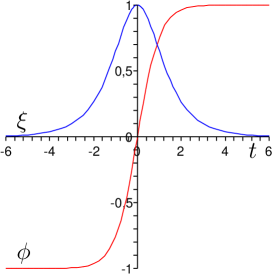
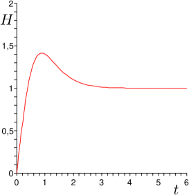
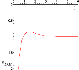
Figure 1: The fields $\phi$ and $\xi$ (left), the Hubble parameter $H$ (center) and the state parameter $w_{DE}$ (right) at $C=0$ and $t_{1}=0$.

For arbitrary $C$ the Hubble parameter is as follows:

$$\begin{split}H&=\frac{A^{2}\omega\left(e^{\omega(t_{0}-t)}+\left(C^{2}+4A^{2}\right)e^{\omega(t-t_{0})}\right)}{6m_{p}^{2}\left(e^{\omega(t_{0}-t)}+2C+\left(C^{2}+4A^{2}\right)e^{\omega(t-t_{0})}\right)^{3}}\Bigl{(}e^{2\omega(t_{0}-t)}+6Ce^{\omega(t_{0}-t)}+{}\\ &{}+10\left(C^{2}+4A^{2}\right)+6C\left(C^{2}+4A^{2}\right)e^{\omega(t-t_{0})}+\left(C^{2}+4A^{2}\right)^{2}e^{2\omega(t-t_{0})}\Bigr{)}.\end{split}$$ (41)

The straightforward calculations give that for all $C$, but $C=\pm 2A$, $\dot{H}(t)=0$ at four points

$$t_{m_{k}^{\vphantom{27}}}=t_{0}-\frac{1}{\omega}\ln\left(-\frac{4A^{2}+C^{2}\pm 2A\sqrt{8A^{2}+2C^{2}}}{(C\pm 2A)(C^{2}+4A^{2})}\right),\qquad k=1,\dots,4,$$ (42)

where two signs ”$\pm$” are independent. Note that if $C\neq\pm 2A$, then $\ddot{H}(t_{m_{k}^{\vphantom{27}}})\neq 0$. Therefore, the Hubble parameter $H(t)$ has extrema at points $t_{m_{k}^{\vphantom{27}}}$.

At $C>2A$ all four points $t_{m_{k}^{\vphantom{27}}}$ do not belong to real axis.

If $C=2A$, then $\dot{H}(t)=0$ at two points, which do not belong to real axis:

$$\tilde{t}_{m_{1}^{\vphantom{27}}}=t_{0}-\frac{1}{\omega}\ln(-2A)\qquad\mbox{and}\qquad\tilde{t}_{m_{2}^{\vphantom{27}}}=t_{0}-\frac{1}{\omega}\ln(-4A).$$ (43)

So, at $C\geqslant 2A$ the Hubble parameter $H(t)$ is a monotonically increasing function and its behavior is close to the behavior of the Hubble parameter in one-field model [9].

At $-2A<C<2A$ the function $H(t)$ has extrema at two points. If $t_{1}=0$, the $\phi(t)$ is an odd function, whereas $\xi(t)$ is an even one. Therefore the corresponding Hubble parameter, calculated by means of (27), is an odd function. It is easy to check that on semi-axis $t>0$ the Hubble parameter $H(t)$ is positive and, hence, has a maximum at $C<2A$ (see Figure 2). Thus, the behavior of $H(t)$ in the case $-2A<C<2A$ looks like its behavior at $C=0$.

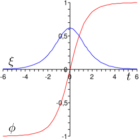
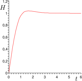
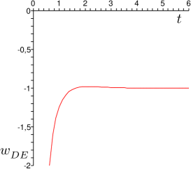
Figure 2: The fields $\phi$ and $\xi$ (left), the Hubble parameter $H$ (center) and the state parameter $w_{DE}$ (right) at $C=1$ and $t_{1}=0$.

If $C=-2A$, then $\dot{H}(t)=0$ at two points:

$$\tilde{t}_{m_{3}^{\vphantom{27}}}=t_{0}-\frac{1}{\omega}\ln(2A)\qquad\mbox{and}\qquad\tilde{t}_{m_{4}^{\vphantom{27}}}=t_{0}-\frac{1}{\omega}\ln(4A).$$ (44)

At these points $\ddot{H}=\pm 16A^{2}/m_{p}^{2}\neq 0$, hence, the Hubble parameter behavior is close to $H(t)$ on Figures 1 and 2.

Let us consider the case $C<-2A$. All four points of extremum (42) are real. It means, that at $C<-2A$ we obtain a qualitative new behavior of the Hubble parameter.

If $t_{1}=0$, then, as it has been noted above, the Hubble parameter is an odd function. The derivative of the Hubble parameter at zero point is positive, hence, $H(t)$ has maximum at some point $t_{m_{1}}>0$, a minimum at $t_{m_{2}}>t_{m_{1}}$ and is a monotonically increasing function at $t>t_{m_{2}}$. Note that $w_{DE}^{\vphantom{27}}<-1$ at $t>t_{m_{2}}$. Thus we have found the exact solutions, which correspond to the nonmonotonic function $H(t)$ with phantom large time behaviour (see Figure 3).

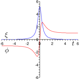
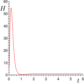
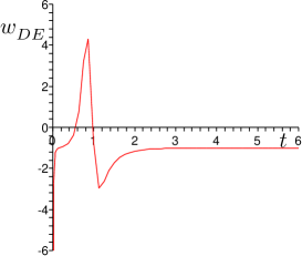
Figure 3: The fields $\phi$ and $\xi$ (left), the Hubble parameter $H$ (center) and the state parameter $w_{DE}$ (right) at $C=-5$ and $t_{1}=0$.

Using the superpotential method we have obtained that the model with the potential

$$\tilde{V}=\omega^{2}\left(\frac{1}{8}\left(1-\phi^{2}+\xi^{2}\right)^{2}-\frac{1}{2A^{2}}\phi^{2}\xi^{2}+\frac{3\phi^{2}}{4m_{p}^{2}}\left(\frac{A}{2}\left(1-\frac{\phi^{2}}{3A^{2}}\right)+\frac{\xi^{2}}{2A}\right)^{2}\right)$$ (45)

has two-parameter sets of exact solutions. Note that the obtained solutions have one and the same asymptotic conditions, whereas the behaviour of the state parameter $w_{DE}^{\vphantom{27}}$ turn out different. So, we can conclude that at large time both quintessence ($w_{DE}^{\vphantom{27}}>-1$) and phantom ($w_{DE}^{\vphantom{27}}<-1$) behavior of $w_{DE}^{\vphantom{27}}$ are possible to obtain from the SFT inspired effective model with one and the same polynomial potential.

6 Two-fields model with a polynomial potential and $w_{DE}$ crossing the cosmological barrier infinitely often

From the Cubic Superstring Field Theory I.Ya. Aref’eva and A.S. Koshelev obtained that the late time rolling of non-local tachyon leads to a cosmic acceleration with a periodic crossing of the cosmological constant barrier [14]. At large time approximation, when an open string tachyon $\phi=1-\tilde{\delta\phi}$ and $|\tilde{\delta\phi}|\ll 1$, the following Hubble parameter has been obtained:

$$H=H_{0}+C_{H}^{\vphantom{27}}e^{-2rt}\sin(2\nu(t-t_{0})),$$ (46)

where $H_{0}$, $C_{H}^{\vphantom{27}}$, $r$, $\nu$ and $t_{0}$ are real constants.

In [14] the authors consider non-local model and the corresponding Friedmann equations. In this paper we construct the two-fields local model with the Hubble parameter (46) in the case $\nu=r$. For simplicity we put $C_{H}^{\vphantom{27}}=1/(2m_{p}^{2})$ and construct solutions, which do not depend on $m_{p}^{2}$. In this case

$$\dot{H}=\frac{r}{m_{p}^{2}}e^{-2rt}\Bigl{(}2\sin(rt)^{2}-(\sin(rt)-\cos(rt))^{2}\Bigr{)}.$$ (47)

Using (4) we can define the following explicit form of solutions:

$$\dot{\tilde{\delta\phi}}={}-2\sqrt{r}e^{-rt}\sin(rt),\qquad\dot{\xi}=\sqrt{2r}e^{-rt}\Bigl{(}\sin(rt)-\cos(rt)\Bigr{)}.$$ (48)

It is easy to check that if

$$\tilde{\delta\phi}=\frac{1}{\sqrt{r}}e^{-rt}\Big{(}\cos(rt)+\sin(rt)\Big{)},\qquad\xi={}-\frac{\sqrt{2}}{\sqrt{r}}e^{-rt}\sin(rt),$$ (49)

then

$$\dot{\tilde{\delta\phi}}=\sqrt{2}r\xi,\qquad\dot{\xi}={}-\sqrt{2}r\tilde{\delta\phi}+2r\xi.$$ (50)

Let construct the superpotential:

$$\frac{\partial W}{\partial\tilde{\delta\phi}}=\frac{1}{2m_{p}^{2}}\sqrt{2}r\xi,\qquad\frac{\partial W}{\partial\xi}=\frac{1}{2m_{p}^{2}}\left(\sqrt{2}r\tilde{\delta\phi}-2r\xi\right),$$ (51)

so

$$W=\frac{1}{2m_{p}^{2}}\left(\sqrt{2}r\xi\tilde{\delta\phi}-r\xi^{2}\right)+H_{0}.$$ (52)

The potential is (we put $H_{0}=0$)

$$V=-r^{2}\left(\xi^{2}+\tilde{\delta\phi}^{2}-2\sqrt{2}\xi\tilde{\delta\phi}\right)+\frac{3r^{2}}{4m_{p}^{2}}\left(\sqrt{2}\xi\tilde{\delta\phi}-\xi^{2}\right)^{2}.$$ (53)

Thus we obtain the explicit solutions and the fourth degree polynomial potential, which corresponds to the Hubble parameter from the SFT inspired model with high derivatives.

Note that the standard method to construct models with scalar fields for the given behaviour of the Hubble parameter is the method, which uses $V(\phi,\xi)$ as a function of time [13]. If we know the Hubble parameter $H(t)$, then, using (9), we obtain $V(t)$ and after that we can attempt to find the functions $\phi(t)$ and $\xi(t)$ and the potential $V(\phi,\xi)$. Such method is very effective if at least one of derivatives either $V_{\phi}$ or $V_{\xi}$ is such a function $F(V)$ that a form of $F$ does not depend on $\phi$ and $\xi$. For example, if

$$V(\phi,\xi)=V_{1}(\phi)e^{\alpha\xi},$$ (54)

where $\alpha$ is a constant, then

$$\frac{\partial V(\phi(t),\xi(t))}{\partial\xi}=\alpha V_{1}(\phi(t))e^{\alpha\xi(t)}=\alpha V(t)$$ (55)

and (6) is a linear differential equation in $\xi$

$$\ddot{\xi}+3H(t)\dot{\xi}+\alpha\left(3H^{2}(t)+\dot{H}(t)\right)=0.$$ (56)

This equation allows to find $\xi(t)$ if the Hubble parameter $H(t)$ is known [13]. The superpotential method is not so effective to seek potential in the form (54) for the given Hubble parameter $H(t)$. On the other hand if the required form of the potential is a polynomial, the superpotential method is not less effective and maybe even more easy to use than the above-mentioned method.

7 Conclusions

In this paper we have investigated the dynamics of two component DE models, with one phantom field and one usual field. The main motivation for us is a model of the Universe as a slowly decaying D3-brane, whose dynamics is described by a tachyon field [17]. To take into account the back reaction of gravity we add a scalar field with an usual kinetic term.

We construct a cosmological model with the SFT inspired polynomial potential $V(\phi,\xi)$ and find two-parameter set of exact solutions. This set can be separated into two subset such that one subset corresponds to the quintessence large time behaviour, another subset corresponds to the phantom one. Note that both subsets have solutions, which satisfy one and the same asymptotic conditions and the additional condition $\phi(0)=0$.

We also construct two-fields model with the fourth degree polynomial potential, which corresponds to the Hubble parameter, obtained in the SFT framework [14]. In this model the state parameter $w_{DE}$ crosses the cosmological constant barrier infinitely often.

In this paper we actively use the superpotential method and show that there are new ways to use this method in the case of two fields. We can not only construct potential for the given solutions, but also find new solutions. In particular superpotential method allows to generalize a one-parameter set of solutions up to two-parameter set. The superpotential method allows to separate the initial system of motion equations (3)–(6) into two parts. One part is the equation on superpotential (15), which in general case is not integrable, but for many polynomial potentials has special solutions. Substituting these solutions into the second part (system (13)–(14)) we obtain a system of ordinary differential equations, which is usually integrable at least in quadratures. Note that the systems of the type (13)–(14) are actively investigated both in mechanics and in supersymmetry theories with BPS states. So, the superpotential method allows to stand out from the system of the Friedmann equations a subsystem, which can be integrable, even in the case of a nonintegrable initial system. On the other hand this method allows to make such a fine tuning of parameters of the considering gravitational models, for example, a choose of coefficients of the potential, that the explicit solutions exist.

For solutions with $H(0)=0$ we obtain that $\dot{H}(0)>0$. Similar solutions are known as bounce ones (see, for example, [43]). Note, that bounce solutions has been obtained in the SFT inspired higher-derivative models [44, 45].

References

- [1] A. Riess et al. [Supernova Search Team Collaboration], Observational Evidence from Supernovae for an Accelerating Universe and a Cosmological Constant, Astron. J. 116 (1998) 1009–1038; astro-ph/9805201.
- [2] D.N. Spergel et al. [WMAP Collaboration], First Year Wilkinson Microwave Anisotropy Probe (WMAP) Observations: Determination of Cosmological Parameters, Astroph. J. Suppl. 148 (2003) 175–194; astro-ph/0302209, D.N. Spergel et al. [WMAP Collaboration], Wilkinson Microwave Anisotropy Probe (WMAP) Three Year Results: Implications for Cosmology, Astrophys. J. Suppl. Ser. 170 (2007) 377–408; astro-ph/0603449.
- [3] Tegmark et al. [SDSS Collaboration], Cosmological parameters from SDSS and WMAP, Phys. Rev. D69 (2004) 103501; astro-ph/0310723.
- [4] P. Astier et al. [SNLS Collaboration], The Supernova Legacy Survey: Measurement of , and from the First Year Data Set, Astron. Astrophys. 447 (2006) 31–48; astro-ph/0510447.
- [5] E.J. Copeland, M. Sami, Sh. Tsujikawa, Dynamics of dark energy, Int. J. Mod. Phys. D15 (2006) 1753–1936, hep-th/0603057
- [6] Y. Gong, A. Wang, Reconstruction of the deceleration parameter and the equation of state of dark energy, astro-ph/0612196.
- [7] U. Alam, V. Sahni, A.A. Starobinsky, Exploring the Properties of Dark Energy Using Type Ia Supernovae and Other Datasets, JCAP 0702 (2007) 011, astro-ph/0612381
- [8] V. Sahni, A.A. Starobinsky, Reconstructing Dark Energy, Int. J. Mod. Phys. D15 (2006) 2105–2132, astro-ph/0610026.
- [9] I.Ya. Aref’eva, A.S. Koshelev, S.Yu. Vernov, Exact Solvitions in a String Cosmological Model, Theor. Math. Phys. 148 (2006) 895–909 [Teor. Mat. Phys. 148 (2006) 23–41]; astro-ph/0412619.
- [10] U. Alam, V. Sahni, T.D. Saina A.A. Starobinsky, Is there Supernova Evidence for Dark Energy Metamorphosis?, Mon. Not. Roy. Astron. Soc. 354 (2004) 275; astro-ph/0311364
- [11] A. Vikman, Can dark energy evolve to the Phantom?, Phys. Rev. D 71 (2005) 023515; astro-ph/0407107.
- [12] Sh. Nojiri, S.D. Odintsov, Modified gravity and its reconstruction from the universe expansion history, hep-th/0611071, Sh. Nojiri, S.D. Odintsov, The new form of the equation of state for dark energy fluid and accelerating universe, Phys. Lett. B639 (2006) 144–150; hep-th/0606025, Sh. Nojiri, S.D. Odintsov, Unifying phantom inflation with late-time acceleration: scalar phantom-non-phantom transition model and generalized holographic dark energy, Gen. Rel. Grav. 38 (2006) 1285–1304; hep-th/0506212, Sh. Nojiri, S.D. Odintsov, Inhomogeneous equation of state of the universe: phantom era, future singularity and crossing the phantom barrier, Phys. Rev. D72 (2005) 023003; hep-th/0505215, Sh. Nojiri, S.D. Odintsov, Sh. Tsujikawa, Properties of singularities in (phantom) dark energy universe, Phys. Rev. D71 (2005) 063004; hep-th/0501025, Sh. Tsujikawa 2005, Reconstruction of general scalar-field dark energy models, Phys. Rev. D72 (2005) 083512; astro-ph/0508542, S. Nesseris, L. Perivolaropoulos, Crossing the Phantom Divide: Theoretical Implications and Observational Status, JCAP 0701 (2007) 018; astro-ph/0610092, R. Gannouji, D. Polarski, A. Ranquet, A.A. Starobinsky, Scalar-Tensor Models of Normal and Phantom Dark Energy, J. Cosmol. Astropart. Phys. 0609 (2006) 016; astro-ph/0606287, V.A. Rubakov, Phantom without UV pathology, Theor. Math. Phys. 149 (2006) 1651–1664 (Teor. Mat. Fiz. 149 (2006) 409–426), hep-th/0604153, H. Mohseni Sadjadi, M. Alimohammadi, Cosmological coincidence problem in interacting dark energy models, Phys. Rev. D74 (2006) 103007; gr-qc/0610080, M. Alimohammadi, H. Mohseni Sadjadi, The crossing of the quintom model with arbitrary potential, gr-qc/0608016, H. Mohseni Sadjadi, M. Alimohammadi, Transition from quintessence to phantom phase in quintom model, Phys. Rev. D74 (2006) 043506; gr-qc/0605143, P.S. Apostolopoulos, N. Tetradis, Late acceleration and crossing in induced gravity, Phys. Rev. D74 (2006) 064021; hep-th/0604014, V. Sahni, Yu. Shtanov, Brane World Models of Dark Energy, JCAP 11 (2003) 014, astro-ph/0202346, Wen Zhao, Yang Zhang, The Quintom Models with State Equation Crossing , Phys. Rev. D73 (2006) 123509; astro-ph/0604460, Bo Feng, Xiulian Wang, Xinmin Zhang, Dark Energy Constraints from the Cosmic Age and Supernova, Phys. Lett. B607 (2005) 35–41; astro-ph/0404224, Zong-Kuan Guo, Yun-Song Piao, Xinmin Zhang, Yuan-Zhong Zhang, Cosmological Evolution of a Quintom Model of Dark Energy, Phys. Lett. B608 (2005) 177–182; astro-ph/0410654, Xiao-Fei Zhang, Hong Li, Yun-Song Piao, Two-field models of dark energy with equation of state across , Mod. Phys. Lett. A21 (2006) 231–242; astro-ph/0501652, Ming-zhe Li, Bo Feng, Xin-min Zhang, A single scalar field model of dark energy with equation of state crossing , hep-ph/0503268, Hrv. Stefancic, Dark energy transition between quintessence and phantom regimes — an equation of state analysis, Phys. Rev. D71 (2005) 124036; astro-ph/0504518, Rong-Gen Cai, Hong-Sheng Zhang, Anzhong Wang, Crossing in Gauss-Bonnet Brane World with Induced Gravity, Commun. Theor. Phys. 44 (2005) 948–954; hep-th/0505186, Yi-Fu Cai, Hong Li, Yun-Song Piao, Xinmin Zhang, Cosmic Duality in Quintom Universe, gr-qc/0609039, Xin Zhang, Dynamical vacuum energy, holographic quintom, and the reconstruction of scalar-field dark energy, Phys. Rev. D74 (2006) 103505; astro-ph/0609699. Hongsheng Zhang, Zong-Hong Zhu, Crossing by a single scalar on a Dvali-Gabadadze-Porrati brane, Phys.Rev. D75 (2007) 023510, astro-ph/0611834
- [13] A.A. Andrianov, F. Cannata, A.Yu. Kamenshchik, Complex Lagrangians and phantom cosmology, J. Phys. A39 (2006) 9975–9982; gr-qc/0604126.
- [14] I.Ya. Aref’eva, A.S. Koshelev, Cosmic acceleration and crossing of barrier in non-local Cubic Superstring Field Theory model, JHEP 0702 (2007) 041; hep-th/0605085
- [15] V.K. Onemli, R.P. Woodard, Super-Acceleration from Massless, Minimally Coupled , Class. Quantum Grav. 19 (2002) 4607; gr-qc/0204065, S.M. Carroll, M. Hoffman, M. Trodden, Can the dark energy equation-of-state parameter be less than ?, Phys. Rev. D68 (2003) 023509; astro-ph/0301273. St.D.H. Hsu, A. Jenkins, M.B. Wise, Gradient instability for , Phys. Lett. B597 (2004) 270–274; astro-ph/0406043, R.V. Buniy, St.D.H. Hsu, B.M. Murray, The null energy condition and instability, Phys. Rev. D74 (2006) 063518, hep-th/0606091 B. McInnes, Phantom Divide in String Gas Cosmology, Nucl. Phys. B718 (2005) 55–82; hep-th/0502209 V. Gorini, A.Yu. Kamenshchik, U. Moschella, V. Pasquier, A.A. Starobinsky, Stability properties of some perfect fluid cosmological models, Phys. Rev. D72 (2005) 103518; astro-ph/0504576. E.O. Kahya, V.K. Onemli, Quantum Stability of a Phase of Cosmic Acceleration, Phys. Rev. D76 (2007) 043512, gr-qc/0612026.
- [16] I.Ya. Aref’eva, I.V. Volovich, On the Null Energy Condition and Cosmology, hep-th/0612098.
- [17] I.Ya. Aref’eva, Nonlocal String Tachyon as a Model for Cosmological Dark Energy, AIP Conf. Proc. 826 (2006) 301–311, astro-ph/0410443.
- [18] K. Ohmori, A Review on Tachyon Condensation in Open String Field Theories, hep-th/0102085; I.Ya. Aref’eva, D.M. Belov, A.A. Giryavets, A.S. Koshelev, P.B. Medvedev, Noncommutative Field Theories and (Super)String Field Theories, hep-th/0111208; W. Taylor, Lectures on D-branes, tachyon condensation and string field theory, hep-th/0301094.
- [19] I.Ya. Aref’eva, A.S. Koshelev, S.Yu. Vernov, Crossing of the Barrier by D3-brane Dark Energy Model, Phys. Rev. D72 (2005) 064017; astro-ph/0507067.
- [20] I.Ya. Aref’eva, L.V. Joukovskaya, Time Lumps in Nonlocal Stringy Models and Cosmological Applications, J. High Energy Phys. 0510 (2005) 087; hep-th/0504200.
- [21] L.V. Joukovskaya, Ya.I. Volovich, Energy Flow from Open to Closed Strings in a Toy Model of Rolling Tachyon, math-ph/0308034.
- [22] I.Ya. Aref’eva, A.S. Koshelev, S.Yu. Vernov, Stringy Dark Energy Model with Cold Dark Matter, Phys. Lett. B628 (2005) 1–10; astro-ph/0505605.
- [23] I.Ya. Aref’eva, A.S. Koshelev, S.Yu. Vernov, Exact Solutions in SFT Inspired Cosmological Models, Bulgarian J. of Phys., 33, Suppl. 1a (2006) 360–367.
- [24] I.Ya. Arefeva, D.M. Belov, A.S. Koshelev, P.B. Medvedev, Tachyon condensation in cubic superstring field theory, Nucl. Phys B638 (2002) 3–20; hep-th/0011117.
- [25] I.Ya. Arefeva, D.M. Belov, A.S. Koshelev, P.B. Medvedev, Gauge invariance and tachyon condensation in cubic superstring field theory, Nucl. Phys B638 (2002) 21–40; hep-th/0107197.
- [26] E. Witten, Noncommutative geometry and string field theory, Nucl. Phys. B268 (1986) 253–294; E. Witten, Interacting field theory of open superstrings, Nucl.Phys. B276 (1986) 291–324.
- [27] I.Ya. Aref’eva, P.B. Medvedev, A.P. Zubarev, Background formalism for superstring field theory, Phys. Lett. B240 (1990) 356–362; C.R. Preitschopf, C.B. Thorn, S.A. Yost, Superstring Field Theory, Nucl. Phys. B337 (1990) 363–433; I.Ya. Aref’eva, P.B. Medvedev, A.P. Zubarev, New representation for string field solves the consistency problem for open superstring field, Nucl. Phys. B341 (1990) 464–498.
- [28] N. Berkovits, A. Sen, B. Zwiebach, Tachyon Condensation in Superstring Field Theory, Nucl. Phys. B587 (2000) 147–178, hep-th/0002211.
- [29] I.Ya. Aref’eva, L.V. Joukovskaya, A.S. Koshelev, Time Evolution in Superstring Field Theory on non-BPS brane. Rolling Tachyon and Energy-Momentum Conservation, hep-th/0301137. I.Ya. Aref’eva, Rolling tachyon in NS string field theory, Fortschr. Phys. 51 (2003) 652–657.
- [30] K. Ohmori, Toward open closed string theoretical description of rolling tachyon, Phys. Rev. D69 (2004) 026008; hep-th/0306096.
- [31] B. Zwiebach, Oriented open-closed string theory revisited, Annals Phys. 267 (1998) 193–248; hep-th/9705241
- [32] O. DeWolfe, D.Z. Freedman, S.S. Gubser, A. Karch, Modeling the fifth dimension with scalars and gravity, Phys. Rev. D62 (2000) 046008, hep-th/9909134.
- [33] A.G. Muslimov, On the Scalar Field Dynamics in a Spatially Flat Friedman Universe, Class. Quant. Grav. 7 (1990) 231–237.
- [34] D.S. Salopek, J.R. Bond, Nonlinear evolution of long-wavelength metric fluctuations in inflationary models, Phys. Rev. D42 (1990) 3936–3962.
- [35] A.R. Liddle, D.H. Lyth, Cosmological Inflation and Large-scale Structure, Cambridge, NY, 2000.
- [36] D. Bazeia, M.J. dos Santos, R.F. Ribeiro, Solitons in systems of coupled scalar fields, Phys. Lett. A208 (1995) 84–88; hep-th/0311265.
- [37] D. Bazeia, F.A. Brito, Bags, junctions, and networks of BPS and non-BPS defects, Phys. Rev. D61 (2000) 105019; hep-th/9912015.
- [38] A. Brandhuber, K. Sfetsos, Non-standart compatifications with mass gaps ans Newton’s law, J. High Energy Phys. 9910 (1999) 013; hep-th/9908116.
- [39] E.B. Bogomol’nyi, Stability Of Classical Solutions, Sov. J. Nucl. Phys. 24 (1976) 449, Yad. Fiz. 24 (1976) 861–870.
- [40] D. Bazeia, C.B. Gomes, L. Losano, R. Menezes, First-order formalism and dark energy, Phys. Lett. B633 (2006) 415–419; astro-ph/0512197; D. Bazeia, L. Losano, J.J. Rodrigues, First-order formalism for scalar field in cosmology, hep-th/0610028
- [41] D. Bazeia, L. Losano, R. Rosenfeld, First-order formalism for dust, astro-ph/0611770
- [42] A.S. Mikhailov, Yu.S. Mikhailov, M.N. Smolyakov, I.P. Volobuev, Constructing stabilized brane world models in five-dimensional Brans-Dicke theory, Class. Quantum Grav. 24 (2007) 231–242; hep-th/0602143.
- [43] Yi-Fu Cai, Taotao Qiu, Yun-Song Piao, Mingzhe Li, Xinmin Zhang, Bouncing universe with quintom matter, arXiv:0704.1090.
- [44] T. Biswas, A. Mazumdar, W. Siegel, Bouncing Universes in String-inspired Gravity, JCAP 0603 (2006) 009; hep-th/0508194
- [45] I.Ya. Aref’eva, L.V. Joukovskaya, S.Yu. Vernov, Bouncing and Accelerating Solutions in Nonlocal Stringy Models, J. High Energy Phys. 0707 (2007) 087; hep-th/0701184.