Comparing different approaches to model the rotational modulation of the Sun as a star

Abstract

Context. The space missions MOST, COROT and Kepler are going to provide us with high-precision optical photometry of solar-like stars with time series extending from tens of days to several years. They can be modelled to obtain information on stellar magnetic activity by fitting the rotational modulation of the stellar flux produced by the brightness inhomogeneities associated with photospheric active regions.

Aims. The variation of the total solar irradiance provides a good proxy for those photometric time series and can be used to test the performance of different spot modelling approaches.

Methods. We test discrete spot models as well as maximum entropy and Tikhonov regularized spot models by comparing the reconstructed total sunspot area variation and longitudinal distributions of sunspot groups with those actually observed in the Sun along activity cycle 23. Appropriate statistical methods are introduced to measure model performance versus the timescale of variation.

Results. The maximum entropy regularized spot models show the best agreement with solar observations reproducing the total sunspot area variation on time scales ranging from a few months to the activity cycle, although the model amplitudes are affected by systematic errors during the minimum and the maximum activity phases. The longitudinal distributions derived from the models compare well with the observed sunspot group distributions except during the minimum of activity, when faculae dominate the rotational modulation. The resolution in longitude attainable through the spot modelling is $\sim 60^{\circ}$, on average.

Conclusions. The application of the maximum entropy modelling to solar analogues will provide us with a quite detailed picture of their photospheric magnetic activity that can be the base for comparative and evolutionary studies of solar-like magnetic activity and irradiance variations.

1 Introduction

The Total Solar Irradiance (TSI) has been monitored for almost three decades by radiometers that obtained a measure of the bolometric disk-integrated flux of our star. It shows a complex variability with timescales ranging from a few minutes to the eleven year cycle, the origin of which is still not completely understood (see, e.g., Fröhlich & Lean, 2004). The peak-to-peak relative amplitude of the long-term change along the activity cycle is of about 1000 parts per million (ppm) with the maximum irradiance attained at the maximum of activity, whereas the transits of the largest sunspot groups across the solar disk produce irradiance dips with amplitudes up to 3000 ppm that last for $10-15$ days.

Recent investigations have shown that at least 90% of the irradiance variability on time scales from a few days up to the 11-yr cycle can be accounted for by the brightness inhomogeneities produced by surface magnetic fields, specifically by cool sunspots and warm faculae (e.g., Krivova et al., 2003; de Toma et al., 2004; Wenzler et al., 2005).

The study of the solar irradiance variability is limited by the lack of similar observations for other main-sequence late-type stars because the current photometric accuracy from the ground is only of $\sim 0.01$ mag (i.e., $\sim 10^{4}$ ppm), allowing us to study the variability only for objects younger than a few hundreds Myr (e.g., Messina & Guinan, 2002). Only for the seasonal averages of the optical magnitudes, it is possible to reach an accuracy of the order of a few $10^{3}$ ppm from the ground (cf., e.g., Radick et al., 1998).

The situation is going to change thanks to the space-borne photometric experiments already in operation (MOST) or planned for the near future (COROT and Kepler). The Microvariability and Oscillations of STars (MOST) satellite can reach a photometric accuracy of $50-100$ ppm in 100-min integration time on bright stars ($3<V<6$) observing a single target in a passband between 350 and 700 nm for time intervals up to 30-40 days (Walker et al., 2003; Croll et al., 2006).

The space mission COROT (COnvection, ROtation and Transits) will simultaneously observe between 6,000 and 12,000 stars with $12<V<16$, in selected fields of view, for time intervals up to 150 days to look for planetary transits. The time series obtained will have a sampling of 8 min and will reach a photometric accuracy of $100-200$ ppm in one hour integration time for stars of apparent magnitude $V\sim 12-13$. For stars brighter than $V=14$, COROT will also recover information on the spectral distribution of the optical flux. For fainter stars, an integrated measure in the passband $350-1000$ nm will be available (Baglin, 2003; Moutou et al., 2005).

Kepler is a mission that will continuously observe a field in the constellation of the Cygnus for at least 4 years, simultaneously monitoring the flux variations in the passband $400-900$ nm for about 100,000 stars with a 15-min time sampling. The photometric accuracy is of 20 ppm for an integration time of 6.5 hours on a G2V star of $V=12$ (Borucki et al., 2004).

Although the photometry obtained by such experiments will be limited to the optical band, they will provide us with data to investigate the irradiance variations of a large sample of solar-like stars. Photospheric cool spots and warm faculae are expected to dominate variations in the optical passband, as it is indeed observed in the Sun, although a significant contribution to the total irradiance variation of our star comes also from the ultraviolet domain (Unruh et al., 1999; Krivova et al., 2003).

In the case of the Sun, it is possible to model the irradiance variations by summing up the flux perturbations produced by each active region observed on the solar disk at a given time (see, e.g., Chapman, 1987; Fligge et al., 1998; Krivova et al., 2003). The same approach cannot be applied to distant stars because of the lack of spatial resolution. Tomographic techniques based on high-resolution spectroscopy, such as the classic Doppler imaging method, are applicable only to fast rotators (${\rm v}\sin i\geq 20-25$ km s^-1; cf., e.g., Strassmeier, 2002).

In the case of slowly rotating solar analogues, the modelling of the irradiance variations must be based on the information on the location and area of the surface active regions provided by the rotational modulation of the stellar flux. Assuming that the active regions are stable during their transit across the disk of a star as it rotates, the variability of the optical flux can be attributed to the modulation of the visibility of the active region themselves. In the framework of this hypothesis, we can obtain a map of the filling factor of the active regions over the surface of a star, independently of its rotation period, as it has been done for several very active late-type stars. Earlier models were based on two circular spots whose co-ordinates and radii were adjusted in order to fit the light curve rotational modulation (see, e.g., Rodonò et al., 1986). The same kind of approach, but using three active regions containing cool spots and bright faculae in a fixed proportion, was applied by Lanza et al. (2003) and Lanza et al. (2004) to fit the total as well as the spectral solar irradiance variations. The position of the three model active regions and the variation of their total area along a significant fraction of activity cycle 23 turned out to be in general agreement with those of the largest observed active regions and complexes of activity dominating the solar irradiance variations. However, in a significant number of cases, the longitudinal distribution of the observed active regions was too much complex to be described with only three active regions and this resulted in a poor agreement between the model and the observations.

A similar situation arises also in the case of the most active stars. The surface maps obtained from the light curve modelling of the K1 subgiant component of the RS CVn system HR 1099 can be compared with the much more detailed Doppler imaging maps revealing that the spot models based on two or a few spots are generally not suited to reconstruct the complex distribution of surface brightness inhomogeneities characterizing a real active star (Vogt et al., 1999). On the other hand, the application of the Maximum Entropy (hereinafter ME) and Tikhonov (hereinafter T) regularization techniques to a continuous distribution of spots, showed a significantly better agreement between the maps based on wide-band photometric data and those obtained by Doppler imaging. In particular, the longitude distribution of the spotted area and its total variation versus time can be safely reconstructed by means of those more sophisticated light curve inversion techniques, as it was shown by Lanza et al. (2006).

In the present paper, we apply the ME and T regularizations to model the total solar irradiance variations treating the Sun as a distant active star, i.e., without introducing any information coming from its spatially resolved observations. The resulting maps of the active region distributions will be compared with the location and the area of the observed sunspot groups to assess the advantages and drawbacks of the proposed spot modelling techniques. A comparison with the results obtained with the previous modelling approach of Lanza et al. (2003) will also be presented.

In this way, we shall test the performance of light curve inversion techniques to be applied for the analysis of the forthcoming high-precision photometric observations of main-sequence late-type stars. Mapping the distribution of their surface brightness inhomogeneities, although with a limited spatial resolution, will be of fundamental importance to understand the basic mechanisms of solar-like activity and variability along the main sequence. This will provide us with a new perspective to consider the fundamental problems of the long and short-term solar irradiance variations, with their impact on the Earth environment and climate, and the physical processes responsible for magnetic field amplification and modulation in the Sun and solar-like stars, i.e., the stellar hydromagnetic dynamo.

2 The time series of the total solar irradiance

We shall model the time series of the TSI obtained by the VIRGO experiment on board of the satellite SoHO. VIRGO has two radiometers to measure the total solar irradiance, DIARAD and PMO6V, each of which has a replica that is exposed to the solar radiation only occasionally to determine the degradation of the one that is in continuous operation. Details on the measurement principle and performance can be found in Fröhlich et al. (1995) and Fröhlich et al. (1997). The measurements are first corrected for all the known instrumental and environmental effects, and reported to 1 AU distance and zero radial velocity, giving the so-called level 1.0 data. The corrections for the instrumental degradation due to the exposure to solar radiation and for long-term non-exposure dependent effects are obtained by comparing the time series of DIARAD and PMO6V with each other and with other experiments simultaneously measuring the TSI. The procedure followed to derive such corrections is described in the VIRGO web site and detailed in Anklin et al. (1999), Fröhlich & Finsterle (2001), Fröhlich (2003) and Crommelynck et al. (2004). In this way, the final TSI time series of level 2.0 is obtained. We retrieved it from the file: virgo_tsi_h_v6_90.dat that is accessible from the VIRGO web site at the Physikalisch-Meteorologisches Observatorium Davos – World Radiation Center. It consists of hourly mean values that range from 7 February 1996 to 28 September 2005 with occasional gaps the length of which is of the order of a few hours or days, except for the four-month gap that occurred in mid 1998, when the spacecraft tracking was lost. The standard deviation of the hourly TSI data is 20 ppm.

3 Models of the solar irradiance variation

The reconstruction of the surface brightness distribution from the inversion of disk-integrated flux values, modulated by stellar rotation, is an ill-posed problem because of the non-uniqueness of the solution and its instability, i.e., small fluctuations in the input data can produce large changes in the map corresponding to the minimum of the $\chi^{2}$. This situation arises because the rotational modulation of the flux is a function of the variation of the surface brightness versus the longitude, while it contains very little information on its latitudinal dependence. When the inclination of the rotation axis is close to $90^{\circ}$, as in the case of the Sun, the duration of the transit of a surface feature across the disk is independent of the latitude (the effect of the surface differential rotation is negligible in this context) and, therefore, no information on its latitude can be extracted from the light curve.

The only quantities that can be safely derived by modelling the rotational modulation of the TSI are the longitudinal distribution of the covering factor of the active regions and the variation of their total area, measured with respect to a reference value corresponding to a given value of the irradiance that we assume to be that of the unperturbed Sun (cf., e.g., Lanza et al., 2003). The contrast of the surface brightness inhomogeneities must be assumed because their temperatures cannot be derived from measurements in a single spectral band. Only when the simultaneous flux modulations in different passbands can be compared, we can estimate the temperatures of the spots and faculae and derive their contrasts (cf., e.g., Lanza et al., 2004; Messina et al., 2006).

In order to overcome the non-uniqueness and the instability of the spot modelling based on light curve inversion, two approaches have been proposed. The first adopts a simple configuration of the brightness inhomogeneities, e.g., it assumes that there are only three active regions, and derives their co-ordinates and areas by fitting the light curve. In the case of the Sun as a star, the rotation period is also included among the free parameters because the short lifetime of the active regions and their random appearance on the solar disk, especially during the phases of high activity of the 11-yr cycle, prevent the precise determination of the rotation frequency from the power spectrum of the TSI variation (see Lanza et al., 2003, 2004).

This modelling approach has the advantage that a limited number of free parameters appears in the model, so that the uniqueness and instability problems are significantly reduced and a meaningful solution can be obtained by minimizing the $\chi^{2}$.

A second approach makes use of regularizing functionals, i.e., of some a priori assumptions on the statistical properties of the brightness map, to derive a unique and stable map of the surface features. In this case, the surface of the star is subdivided into a large number of elements and the covering factors of the active regions within the elements are considered as free parameters. Among the potentially infinite solutions that fit the rotational modulation of the flux, those are selected that maximize the configurational entropy (ME solution) or minimize the Tikhonov functional (T solution) of the map. In this case, the rotation period needs to be fixed at the outset, because of the large number of free parameters that would make its variation impratical in terms of computing time.

The implementation of these approaches is described in some detail below.

3.1 The three-spot model of the TSI variation

The model is described by Lanza et al. (2003), therefore only a brief introduction is given here. It makes use of three active regions, containing both cool spots and warm faculae, to fit the rotational modulation of the TSI, and a uniformly distributed background component to fit the variation of its mean level along the 11-yr cycle. The ratio of the area of the faculae to that of the sunspots in each active region is fixed and is indicated by $Q$. The brightness of the unperturbed photosphere is modelled by a quadratic limb-darkening law:

$$I_{\rm u}(\mu)=\mathcal{C}(a_{\rm p}+b_{\rm p}\mu+c_{\rm p}\mu^{2}),$$ (1)

with $a_{\rm p}=0.36$, $b_{\rm p}=0.84$ and $c_{\rm p}=-0.20$ and $\mathcal{C}\equiv[(1/4)(a_{\rm p}+2b_{\rm p}/3+c_{\rm p}/2)]^{-1}=4.88$ (cf. Lanza et al., 2003).

The contrast between the sunspot and the unperturbed photosphere, as measured by the ratio of their specific intensities, $c_{\rm s}\equiv I_{\rm s}/I_{\rm u}=0.67$, is assumed fixed and independent of the position on the solar disk. The facular contrast is assumed to vary as: $I_{\rm f}/I_{\rm u}=1+c_{\rm f}-c_{\rm f}\mu$, where $c_{\rm f}=0.115$ and $\mu\equiv\cos\psi$, with $\psi$ being the angle between the normal to a given surface element and the line of sight, i.e., its limb angle.

The rotation period $P_{\rm rot}$ is assumed as a free parameter ranging from 23.0 to 33.5 days, and its value is determined, together with the other free parameters, by minimizing the $\chi^{2}$. The inclination of the rotation axis $i$ is held fixed at its true value during the fitting process. The number of free parameters is therefore eleven.

The timescale of evolution of the active region pattern on the Sun is significantly shorter than the rotation period. Therefore, it is not possible to model an entire rotation by adopting a fixed pattern of active regions. The longest time interval that can be modelled with three stable active regions is 14 days (cf. Lanza et al., 2003). Hence, the TSI time series is subdivided into subsets of 14 days, each of which is fitted with the model described above. The lag between the beginning of two consecutively fitted time intervals is fixed at 7.0 days like in Lanza et al. (2003), giving a total of 484 intervals when the gaps in the time series are taken into account.

The time series obtained by MOST and those to be obtained by COROT have an extension ranging from $\sim 30$ to $\sim 150$ days. Therefore, they do not allow us to sample the whole range of stellar irradiance variations along an activity cycle. For this reason, in the present work we compute the best fits assuming as the reference irradiance value (i.e., that corresponding to the unperturbed Sun) the maximum of the TSI along each of the 14-day subsets. This approach differs from that of Lanza et al. (2003) where the observed maximum of the TSI in the $1996.1-2001.6$ interval was adopted as a reference value. The present choice makes the role of the uniformly distributed background component almost irrelevant and the total spotted area comes from the amplitude of the TSI rotational modulation along each 14-day interval.

With this assumption for the reference value, it is found that the parameter $Q$ must be adjusted to the value $Q=9$, instead of the previously adopted $Q=10$ (cf. Lanza et al., 2003) to have residuals with a symmetric distribution around an average zero value. The other parameters adopted for the three-spot modelling are the same as Lanza et al. (2003).

The main limitation of the three-spot model is the low number of degrees of freedom to map the surface of the Sun that cannot account for the very complex active region configuration observed on the photosphere of our star, especially during the phases of moderate or high activity.

3.2 Maximum Entropy and Tikhonov models of the TSI variation

To fit the variations produced by a complex pattern of active regions on the Sun, the best approach is provided by regularized maps. The surface of the star is subdivided into 200 squared elements of side $18^{\circ}$ of latitude whose filling factors are varied to reproduce the rotational modulation of the TSI. Specifically, we consider the filling factors of the unperturbed photosphere, the spotted photosphere and the faculae that are indicated by $q_{\rm u}$, $q_{\rm s}$ and $q_{\rm f}$, respectively, with $q_{\rm u}+q_{\rm s}+q_{\rm f}=1$. The area ratio between the faculae and the sunspots is fixed, i.e., we assume $q_{\rm f}/q_{\rm s}\equiv Q$. In this way, the value of $q_{\rm s}$ for a given element fixes also the values of $q_{\rm f}$ and $q_{\rm u}$ and can be used to specify the active region distribution.

By assuming the same dependence of the contrasts of spots and faculae adopted for the three-spot model (cf. Sect. 3.1), the specific intensity of a surface element at limb angle $\psi$ and with a spot filling factor $q_{\rm s}$ can be written as:

$$I(\mu)=\left\{1+\left[c_{\rm s}-(1+Q)+Q(1+c_{\rm f}-c_{\rm f}\mu)\right]q_{\rm s}\right\}I_{\rm u}(\mu),$$ (2)

where the unperturbed specific intensity is given by Eq. (1).

The contribution of the $i$-th element to the bolometric flux at time $t_{k}$ is:

$$\Delta F_{ik}=A_{i}I[\mu_{i}(t_{k})]\mu_{i}(t_{k})g[\mu_{i}(t_{k})],$$ (3)

where $A_{i}$ is the area of the element, $I$ is the specific intensity given by Eq. (2), $\mu_{i}(t_{k})\equiv\cos\psi_{i}(t_{k})$, with the limb angle $\psi_{i}$ of the element depending on its longitude, latitude and the time $t_{k}$, and $g(\mu)$ is the visibility function, i.e., $g(\mu)=1$ for $\mu>0$, $g(\mu)=0$ for $\mu\leq 0$. To warrant a sufficient precision in the computation of the disk-integrated flux, each surface element is further subdivided into smaller squared elements with side $1^{\circ}$ having the same filling factor $q_{s}$ of the initial element, thus keeping the number of free parameters in our model equal to 200. The bolometric flux at the time $t_{k}$ is given by: $F(t_{k})=\sum_{i}\Delta F_{ik}$.

The reduced $\chi^{2}$ statistic is defined as:

$$\chi^{2}=\frac{1}{M}\sum_{k=1}^{M}\frac{(F_{k}-D_{k})^{2}}{\sigma^{2}},$$ (4)

where $F_{k}\equiv F(t_{k})$ is the computed flux and $D_{k}$ the observed flux at time $t_{k}$, $\sigma$ the standard deviation of the TSI (equal to $2.0\times 10^{-5}$ in relative flux units), and $M$ the number of data points in the fitted subset of the TSI series assumed to have a length of 14 days (cf. Sect. 3.1).

The regularized solutions are computed by a constrained minimization of an objective function that is a linear combination of the reduced $\chi^{2}$ and a regularizing function which accounts for the a priori assumptions on the filling factor map, i.e., on the distribution of $q_{\rm s}$ over the surface of the star. Specifically, the objective functions are:

$$\mathcal{Q}_{\rm ME}=\chi^{2}-\lambda_{\rm ME}S,$$ (5)

for the ME solution, and

$$\mathcal{Q}_{\rm T}=\chi^{2}+\lambda_{\rm T}T,$$ (6)

for the T solution, where the reduced $\chi^{2}$ is given by Eq. (4), $\lambda_{\rm ME}$ and $\lambda_{\rm T}$ are Lagrange multipliers, and $S$ and $T$ are the ME and T regularizing functions the expressions of which are given by Lanza et al. (1998). The procedure of minimization, including the evaluation of the Lagrange multipliers, is described in detail by Lanza et al. (1998) to which we refer the reader. Here we note only that the ME map is characterized by a minimum total spotted area because the value of $q_{\rm s}$ in each surface element is driven toward zero, whereas the T map is characterized by a distribution of the filling factor as smooth as possible, i.e., the regularization drives the map towards that of a uniformly spotted star.

4 Statistics to compare the models with the observations

4.1 Comparison of the modelled and observed TSI variations

Krivova et al. (2003) and Wenzler et al. (2005) compared the observed TSI variations with their models by performing a linear regression between measured and modelled values and found a correlation coefficient of 0.94. This approach can be extended to measure the performance of a given model to reproduce the variation of the TSI at different frequencies by means of bivariate analysis (cf., e.g., Priestley, 1981). We assume a general linear relation between the observed $D(t_{k})$ and the modelled TSI values $F(t_{k})$:

$$D(t_{k})=\sum_{j=-\infty}^{\infty}f(t_{j})F(t_{k-j})+N(t_{k}),$$ (7)

where $f(t_{k})$ is the impulse response function and $N(t_{k})$ the noise at time $t_{k}$, with the time instants assumed to be uniformly spaced by $\Delta t$ (i.e., $t_{k}=k\Delta t$). Equation (7) means that the value of the observed TSI at a given time is a linear combination of all the past, present and future values of the model, with the function $f(t)$ giving a measure of the relative contributions at different time delays. In this way, relation (7) also takes into account a possible delayed (or anticipated) response of our model.

The relationship between the observed and the modelled time series is expressed by the transfer function, that is the Fourier transform of the impulse response function: $\Gamma(\omega)\equiv\sum_{j=-\infty}^{\infty}f(j\Delta t)\exp(-i\omega j\Delta t)$, where $i=\sqrt{-1}$. An ideal model would have $f(0)=1$ and $f(t)=0$, $\forall t\not=0$, i.e., a gain $|\Gamma(\omega)|=1$ and a phase spectrum $\arg{\Gamma(\omega)}=0$ for all frequencies $\omega$. In other words, the model values would directly reproduce the observations without any delayed (or anticipated) contribution at all frequencies.

The generalization of the linear correlation coefficient is the coherency which expresses the degree of linear correlation between the observed and modelled TSI as a function of the frequency. When the modulus of the coherency is close to unity at all frequency, a linear best fit reproduces well the correlation between the two quantities (see Priestley, 1981, for details).

4.2 Comparison of the total areas and longitude distributions of the active regions

To assess the capability of the proposed modelling approaches, it is important to compare the maps of the active region distributions obtained by light curve inversion with the real distributions of the active regions on the Sun. In consideration of the limitations discussed in Sect. 3, the comparison will concern the variation of the total active region area and the distribution of the active regions in longitude. Since the ratio between the facular and the spot areas is fixed in our model, we can consider the total spotted area and its longitudinal distribution as the model quantities to be compared with the observations. A daily record of the sunspot groups observed on the solar disk, reporting their co-ordinates and areas, is provided by the extension of the Greenwich Photoheliographic Results (hereinafter GPR) made available by Hathaway (2006). These data will be used for our comparisons.

It is important to notice that our models are based on subsets of the TSI time series that extend along half a solar rotation, implying that points on the solar surface having different longitudes are in view for different fractions of the 14-day time interval. Therefore, when we compare the model active region areas with the observed GPR areas, we must take into account that the model active regions contribute to the modulation of the TSI only for some fraction of the time. In other words, their areas must be multiplied by this fraction to be consistently compared with the observed areas during the same time interval.

In view of the above considerations, we define the visibility of a point $P$ on the solar surface along a given 14-day time interval as:

$$v(P)=\frac{1}{(t_{2}-t_{1})}\int_{t_{1}}^{t_{2}}\mu(P,t)g[\mu(P,t)]dt,$$ (8)

where $t_{1}$ and $t_{2}$ are the initial and the final instants of the interval with $t_{2}-t_{1}=14$ days, and the functions $\mu$ and $g$ have already been defined above (see Eq. (2) of Lanza et al., 2003, for the dependence of $\mu$ on the co-ordinates of the point $P$).

The comparison of the total area of the sunspots derived from our models with the observations is straightforward once the element area values have been multiplied by their respective visibilities. The comparison of the longitudinal distributions is more complex. In the case of a discrete spot distribution, we define the mean longitude of the active regions taking into account the circular nature of the data, i.e., we associate to each active region of area $a_{j}$, longitude $\lambda_{j}$ and visibility $v_{j}$ a vector $(a_{j}v_{j}\cos\lambda_{j},a_{j}v_{j}\sin\lambda_{j})$ and then compute the resulting vector normalizing it to the total area, i.e.:

$${\bf R}\equiv\left(\frac{1}{\sum_{j}a_{j}v_{j}}\sum_{j}a_{j}v_{j}\cos\lambda_{j},\frac{1}{\sum_{j}a_{j}v_{j}}\sum_{j}a_{j}v_{j}\sin\lambda_{j}\right),$$ (9)

where the summation is extended over the active regions. The mean longitude of the distribution is given by the longitude toward which the resulting vector ${\bf R}$ points. In this way, we can compare the mean longitude of the three model active regions with that of the sunspot groups observed during any given 14-day interval. In place of the visibility, we use the area averaged over the 14-day interval for the observed sunspot groups.

The dispersion of the longitudes of the model active regions around their mean value is not a statistically meaningful quantity when only three active regions are adopted, hence we shall not consider it in our discussion.

On the other hand, the longitudinal distributions of the spotted area obtained by the ME and the T maps are suitable for a detailed comparison with the longitudes of the sunspot groups observed during the same 14-day time intervals. From the regularized maps, the spotted area in $18^{\circ}$ longitude bins can be easily obtained and compared with the same quantity as derived from the observations. However, since the actual longitudinal resolution of our mapping method is certainly larger than $18^{\circ}$, it is more appropriate to compare the distributions with a wider binning, say, $54^{\circ}$ or $72^{\circ}$. Taking into account the circular nature of our data, a longitudinal distribution corresponds to a set of vectors, each having the direction of a given bin and a modulus proportional to the total area in that bin. The correlation between two distributions $a$ and $b$ is measured by the correlation between the two corresponding sets of vectors, e.g., $\{{\bf V}^{a}_{j}\}$ and $\{{\bf V}^{b}_{j}\}$, with $j=1,...,N$, where $N$ is the number of bins. The correlation coefficient can be defined by specifying to the case of circular data (i.e., to two dimensions) the definition given in Fisher & Lee (1986) and Fisher et al. (1987). More precisely, we define the quantity:

$$S({\bf V}^{a}{\bf V}^{b})\equiv\det\left(\begin{array}[]{cc}\sum_{j}X^{a}_{j}X^{b}_{j}&\sum_{j}Y^{a}_{j}X^{b}_{j}\\ \sum_{j}X^{a}_{j}Y^{b}_{j}&\sum_{j}Y^{a}_{j}Y^{b}_{j}\end{array}\right),$$ (10)

where $X^{a}_{j}$ and $Y^{a}_{j}$ are the components of vector ${\bf V}^{a}_{j}$ and $X^{b}_{j}$ and $Y^{b}_{j}$ those of vector ${\bf V}^{b}_{j}$. Then the correlation coefficient between the two sets of vectors, i.e., between the corresponding longitudinal distributions, is given by:

$$\rho\equiv S({\bf V}^{a}{\bf V}^{b})/[S({\bf V}^{a}{\bf V}^{a})S({\bf V}^{b}{\bf V}^{b})]^{1/2},$$ (11)

with $0\leq\rho\leq 1$ in the case of circular data. A correlation coefficient $\rho=1$ indicates a perfect correspondence between the two distributions. For a given correlation coefficient $\hat{\rho}<1$, we can estimate the probability that $\rho$ is higher than $\hat{\rho}$ for the correlation between a given distribution and a random distribution by means of a Monte Carlo method (Fisher et al., 1987). For instance, in Fig. 1 we report the statistics of the values of $\rho$ obtained by correlating several observed distributions with bins of $54^{\circ}$ with the 5040 random distributions obtained by the permutations of each initial one. The probability of having $\rho\geq 0.4$ by a chance correlation is found to be lower than $\sim 0.1$%.

Figure 1: Histogram of the frequency distribution of the correlation coefficient $\rho$, as given by Eq. (11), between several observed longitudinal distributions of the sunspot group area on the Sun and the 5040 random distributions obtained by the permutations of each of them, respectively.

5 Results

The best fits obtained with the three-spot model introduced in Sect. 3.1 and the corresponding $\chi^{2}$ values are comparable with those obtained by Lanza et al. (2003) and are not shown here. The residuals have an approximately Gaussian distribution with a full width at half maximum of $\sim 80$ ppm.

The best fits with the ME and T regularizations are computed for the same time intervals with the same choice for the unperturbed TSI value and $Q=9$ as for the three-spot model. However, the rotation period is fixed at $P_{\rm rot}=27.27$ days in order to avoid an excessively long computation time. The Lagrange multipliers are set at $\lambda_{\rm ME}=300$ and $\lambda_{\rm T}=5\times 10^{5}$ by the criterium that the distributions of the best fit residuals should not deviate from the almost Gaussian distributions obtained for $\lambda_{\rm ME}=0,\lambda_{\rm T}=0$ by more than one standard deviation, i.e., $\sim 50$ ppm (cf., e.g., Lanza et al., 1998). We note that the present Lagrange multipliers are three orders of magnitude higher than those usually adopted to model stellar light curves (cf., e.g., Lanza et al., 1998, 2002). This is a consequence of the much lower value of the standard deviation of the TSI measurements that makes the trial values of the $\chi^{2}$ much higher than those in the stellar cases, so that correspondingly higher Lagrange multipliers are needed to make effective the regularizing terms in Eqs. (5) and (6).

The best fits obtained with the ME and T regularizations are similar to those obtained with the three-spot model and are not shown here. The $\chi^{2}$ values are usually comparable and are always lower than $12$, whereas in the case of the three-spot models $\chi^{2}>12$ in a few cases (cf., e.g., Fig. 5 in Lanza et al., 2003). In order to judge the performance of the different approaches, we plot in Fig. 2 the gain, the phase spectrum and the coherency vs. frequency for the different model best fits with respect to the observed TSI for two time intervals, close to the activity minimum and the maximum of cycle 23, respectively. In addition to the three-spot models, we consider also models with only two spots. The average $\chi^{2}$ value of the three-spot models is $\sim 30$% lower than that of the two-spot models. We see that the gain and the coherency of the two-spot models begin to depart from the unity already for frequencies of $\sim 0.1$ d^-1, while the three-spot models are good up to $\sim 0.2$ d^-1 during the minimum phases. Therefore, we shall not consider the two-spot models any further.

The ME and T models are closely comparable and perform significantly better than the discrete spot models, especially during the phases of higher activity, as indicated by the gain and the coherency close to unity and the phase angle close to zero for frequencies lower than $\sim 0.25$ d^-1. For higher frequencies, the TSI variations cannot be reproduced by any model based on the rotational modulation of a fixed pattern of active regions because short-term irradiance fluctuations are ruled by the growth and decay of small active regions with a lifetime of a few days (cf. Lanza et al., 2003). Small systematic differences in high-frequency residuals between consecutive best fits separated by 7 days may be the cause of the oscillations observed in the plots of the coherencies of the ME and T models for frequencies higher than $0.3$ d^-1.

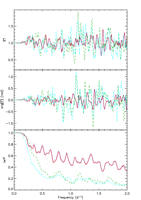
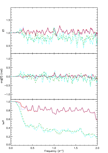
Figure 2: From the upper to the bottom left panels: The gain spectrum $|\Gamma|$, the phase spectrum $\arg{\{\Gamma\}}$ and the square of the modulus of the coherency $|w|^{2}$ versus frequency for our best fit time series versus the observed TSI time series during the interval ranging from 1996.25 to 1997.77. Different linestyles and colors mark different modelling approaches: solid red – ME; dotted blue – T; dashed green – three spots; dash-dotted light blue – two spots. From the upper to the bottom right panels: The same as the left panels for the interval ranging from 1999.52 to 2001.00.

The total spotted areas obtained by the three-spot, the ME and the T models are compared in Fig. 3 with the monthly averaged spotted area in the GPR. It is better to adopt for the comparison the mean model areas along an entire rotation. Thus, the individual values from four consecutive best fits, separated by 7 days each from the other, are averaged.

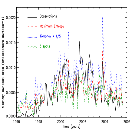
Figure 3: The monthly sunspot group area from the GPR and the averaged model spotted areas, in unit of the entire solar photosphere and corrected for the effects of the visibility, vs. time along activity cycle 23. Note that the values of the areas obtained from the T models have been multiplied by $1/5$ to be plotted on the same scale. Different linestyles and colors mark the various quantities: solid black – observed GPR area; dashed red – ME models; dotted blue – T models; dash-dotted green – three-spot models.

Note that the T models give systematically higher values than the ME models because of their regularizing assumption that smooths the area variation between neighbour surface elements thus increasing the spotted area at high latitudes where its photometric effect is minimum. On the other hand, the ME regularization tends to decrease the spotted area in each surface element as much as possible (see Lanza et al., 1998, for details).

The present results confirm and extend those presented by Lanza et al. (2003), although it is important to mention that the area values reported in that paper are different from ours because of the different assumptions on the TSI reference value. The present model spotted areas are systematically larger than the sunspot group area close to the minimum of activity when the TSI modulation is dominated by the faculae. This happens because our models assume a fixed proportion between the facular and the spotted areas. Hence, when they reproduce the rotational modulation at the cycle minimum they necessarily introduce a certain amount of spotted area. The modulation of the observed spotted area on time scales up to $1-2$ yrs is generally well reproduced by our models, but the amplitude of the overall variation along the activity cycle 23 is somewhat underestimated. To interpret this result, it is useful to look at the plot of the TSI time series along cycle 23 that shows that the amplitude of the TSI monthly variations has remained at approximately the same level from the end of 1999 up to the end of 2004. Since our model spotted areas are derived from the amplitude of the rotational modulation of the TSI, the approximate constancy of their average values in the $2002-2004$ interval reflects the frequent large dips in the TSI time series observed up to the end of 2004. As a matter of fact, cycle 23 was a peculiar one, characterized by two maxima of comparable heights in 2000 and 2002-2003 which delayed the descending phase of the cycle. Our models do not reproduce the amplitude of such maxima, although they follow the shorter-term oscillations of the spotted area occurred during each of them.

These results are confirmed quantitatively by the bivariate analysis of the modelled vs. observed sunspot group areas reported in Fig. 4. The gain spectra show that the ratios of the modelled areas to the observed area depend on the frequency and they are different from unity even at the lowest frequencies. This depends on the different a priori assumptions made on the spot distributions adopted to fit the light curves, as discussed above in the case of the ME and T regularizations.

The regularized models perform significantly better than the three-spot models with the ME models showing the gain closer to unity. It is interesting to note that the ME and T coherencies are lower in the frequency interval corresponding to time scales between 0.25 and 0.8 yr, while their phase angles are significantly different from zero only for timescales between 0.3 and 1.0 yr. For timescales shorter than about 0.25 years, both the coherencies and the phase angles are similar to the values found for timescales longer than one year, indicating that the ME and T models are reproducing the area variation quite well.

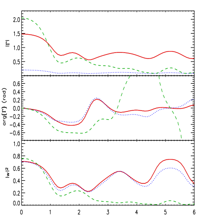
Figure 4: The gain spectrum $|\Gamma|$, the phase spectrum $\arg{\{\Gamma\}}$ and the square of the modulus of the coherency $|w|^{2}$ versus frequency for the modelled area time series vs. the time series of the observed sunspot group area. Different linestyles and colors refer to different modelling approaches: solid red – ME; dotted blue – T; dashed green – three spots.

A discrete spot model based on three spots allows us to define the average longitude of the spotted area distribution (cf. Eq. (9)) which can be compared with the mean longitude of the distribution of the observed sunspot groups during the same 14-day time interval. The comparison statistics are shown in Fig. 5 and indicate that the model mean longitude is within $60^{\circ}$ from the observed mean longitude in 68% of the cases. However, a discrete spot model based on three spots provides only a very rough description of the longitudinal distribution of the spotted area.

Figure 5: The frequency distribution of $\cos\Delta$ for the three-spot models, where $\Delta$ is the angle between the mean longitude of the three model active regions and the mean longitude of the observed sunspot groups as given by Eq. (9). The correction for the visibility effects has been taken into account to compute the mean model longitudes.

The ME and T models, assuming a continuous distribution of the spotted area, give more information. We compare the distribution of the ME model spotted area with the observed distribution of the sunspot group area vs. longitude in the left and right panels of Fig. 6 for selected epochs during the minimum and the maximum of activity cycle 23, respectively. The origin of the longitude reference frame corresponds to the meridian crossing the centre of the solar disk at 23^h 29^m 20^s UT of 6 February 1996 for a geocentric observer. The adopted synodic rotation period of 27.27 days makes the origin of our reference frame drift slowly with respect to the Carrington reference frame with, superposed, a small periodic oscillation of amplitude $\sim 4^{\circ}$ and period of about one year. The value of the area in each longitude bin in Fig. 6 has been normalized to the total spotted area of each distribution, i.e., the sum of the spot area over the bins is always equal to the unity. Such a normalization has been adopted to avoid systematic effects arising from the different total spotted areas of the model and the observations, as discussed above. The correlation coefficients reported in Fig. 6 are computed adopting a bin width of $54^{\circ}$ with the area in each bin obtained by summing up the values of three consecutive bins of $18^{\circ}$. The optimal bin width has been chosen by comparing the correlation coefficients for bin widths of $36^{\circ}$, $54^{\circ}$ and $72^{\circ}$ and selecting the binning that gives the higher resolution and the higher correlation coefficient, on the average. Therefore, a bin width of $54^{\circ}$ corresponds to the average longitudinal resolution of our ME spot modelling technique. Note, however, that the original model bin width of $18^{\circ}$ has been retained for plotting the distributions to show the correlation between models and observations in more detail.

The distributions for the T models are usually broader than those of the ME models implying a lower degree of correlation betweeen the models and the observations and are not reproduced here. During the minimum of activity, the rotational modulation is dominated by the faculae, which implies that our models, having a fixed proportion between the facular and the spotted areas in each surface element, are often not capable of retrieving the correct spot longitudinal distribution. Two cases of such poor agreement are shown in the uppermost left panels of Fig. 6 having a correlation coefficient $\rho$ lower than 0.25. The maximum of activity is characterized by correlation coefficients usually higher than 0.8 indicating a remarkably good agreement between the ME modelled and the observed sunspot group area.

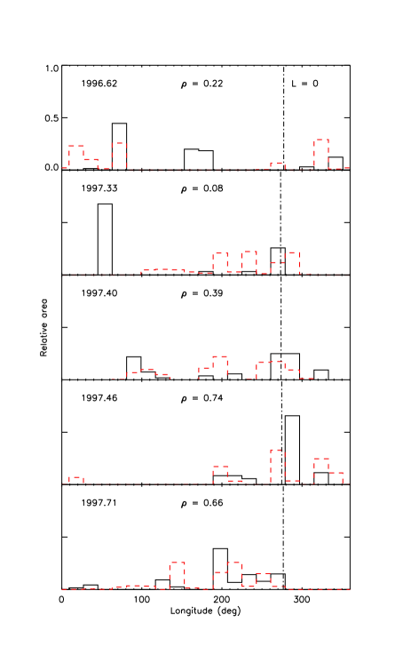
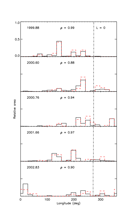
Figure 6: The observed distributions of the sunspot group area (solid black line) and the corresponding ME spot models (dashed red line) vs. longitude binned in $18^{\circ}$ intervals at the labelled epochs, grouping around the minimum of activity cycle 23 in the left column panels and around the maximum in the right column panels, respectively. The modelled distributions are corrected for the effect of the visibility. Both the observed and the modelled distributions are normalized to their total area, respectively. The reference frame is the internal reference frame of our code (see the text). For comparison, the initial meridian of the Carrington reference frame is marked in each panel by a vertically dot-dashed line, labelled $L=0$ in the uppermost panels. The correlation coefficient $\rho$ between the modelled and the observed distributions, as defined by Eq. (11) for longitude bins of $54^{\circ}$, is reported in each panel.

The distribution of the correlation coefficient $\rho$ vs. time is plotted in Fig. 7. The correlation is lower during the phases of lower activity and it is remarkably good during the phases of intermediate or high activity with only a very few values lower than 0.4 during the maximum of cycle 23. As a matter of fact, we see from Figs. 1 and 6 that even a value as low as $\rho=0.4$ indicates a significant degree of correlation between the modelled and the observed distributions.

We have explored the effects of the variations of the model parameters $Q$, $P_{\rm rot}$ and $i$, by changing one parameter at a time while the others are kept fixed. We shall focus our discussion on the ME models because they are those showing the best performance.

It is interesting to consider models with only dark spots, i.e., $Q=0$ because they are analogous to those usually adopted in the case of highly active solar-like stars (cf., e.g., Messina et al., 1999; Lanza et al., 2002, 2006). The $\chi^{2}$ values of the best fits are systematically higher by a factor of about $1.5-2.0$ with more than 10% of the best fits having $\chi^{2}>15$. The total sunspot areas are somewhat smaller than in the reference case ($Q=9$) because smaller spots at the disk center can fit the dips in the TSI modulation, given that the positive irradiance contribution from the faculae closer to the limb is missing. The longitudinal spot distributions are not reproduced as well as in the reference case because the model spot longitudes are modified to reproduce the irradiance modulation due to the faculae which is systematically shifted in phase with respect to that of the sunspots belonging to the same active region.

When $Q$ is increased beyond the value of the reference case, the $\chi^{2}$ values are comparable with those of the reference case up to $Q\sim 15$, but the quality of the fits is significantly degraded for higher $Q$ values. The total model spot areas increase with $Q$ because a larger sunspot area close to the disk center is required to fit the TSI dips given the enhanced contribution of the faculae closer to the limb. The longitude distributions of the spotted area show $\rho$ values that are comparable with those of the reference case up to $Q\sim 15$. For higher values the longitudinal spot distribution is not satisfactorily reproduced by the models.

The rotation period of the Sun cannot be accurately obtained by the analysis of the rotational modulation of the TSI during the phases of moderately high activity or close to the maximum of the 11-yr cycle (cf., e.g., Lanza et al., 2003, 2004). Therefore, we explored the effect of adopting a rotation period shorter by 20% or longer by 20% than the optimal value of 27.27 days, respectively. In both cases, the $\chi^{2}$ values of the best fits are not significantly affected and the variation of the total spotted area vs. time is well reproduced. However, the correlation coefficients $\rho$ between the modelled and the observed longitudinal distributions of the spot area decrease significantly, in other words, the longitudinal resolution of the model is degraded. The systematic error in longitude produced by a relative error $\Delta P/P_{\rm rot}$ in the rotation period is $\sim 180^{\circ}\times\Delta P/P_{\rm rot}$, so that the resolution is degraded by a factor of $\sim 1.5$ with respect to the reference case, when an average value of $50^{\circ}-60^{\circ}$ was found.

Decreasing the inclination angle to fixed values of $60^{\circ}$ and $30^{\circ}$, respectively, produces no significant degradation in the quality of the best fits as indicated by the $\chi^{2}$ values that are comparable with those of the reference case. The total model spot area does not change significantly for $i=60^{\circ}$ and the longitudinal distributions of the model spot area are well comparable with the observed ones, with no significant degradation with respect to the reference case.

Figure 7: The correlation coefficient $\rho$ between the ME spot model and the observed longitudinal sunspot group distributions, as given by Eq. (11) for longitude bins of $54^{\circ}$, vs. time. The model distributions are corrected for the effects of the visibility.

6 Discussion

We have performed a detailed study of the capabilities of different spot modelling techniques to retrieve information on the area variation and longitudinal distribution of active regions through the modelling of the rotational modulation of the solar irradiance along activity cycle 23. Previous studies were limited to the Sun at minimum activity, i.e., characterized by a geometrically simple configuration of the active regions (e.g., Oláh et al., 1999), or did not use quantitative statistical methods to study the correlation between modelled and observed active region distributions (e.g., Lanza et al., 2003). Moreover, e.g., Oláh et al. (1999) and Catalano et al. (1998) did not model the optical flux modulation, but focussed on the flux coming from the corona and the chromosphere, respectively. Those studies are, therefore, more relevant for the modelling of the Sun as a star in the X-ray and UV spectral domains (e.g., Orlando et al., 2004), rather than in the optical band.

We have found that the ME models provide the best representation of the solar active region pattern in the photosphere. This is probably related to the fact that active regions are localized features occupying a very small fraction of the solar surface, a characteristic that matches the a priori assumption of ME models, i.e., that of concentrating the brightness inhomogeneities in a number of surface elements as small as possible (cf., e.g., Lanza et al., 1998, and references therein).

It is important to note that our approach cannot give the absolute area of the sunspot groups but only the variation of the area with respect to a reference level. As a matter of fact, the present study demonstrates that the irradiance reference level need not be fixed, but it can be chosen as the maximum of the TSI along each 14-day data subset. In other words, the amplitude of the rotational modulation along each data subset allows us to extract a good measure of the total spotted area, on the average. The longitudinal distribution of the active regions is also well reproduced by our approach with an average resolution of $\sim 50^{\circ}-60^{\circ}$. This implies that a uniform distribution of active regions or one characterized by variations on smaller longitudinal scales cannot be reproduced by our models. In the case of distant stars, the signal-to-noise ratio will also affect the longitudinal resolution as discussed by, e.g., Lanza et al. (2006) in the case of ground-based observations.

Forthcoming space-borne observations will be limited to $4-5$ years in the case of Kepler or 150 days in the case of COROT. However, short-term cyclic variations of the spotted area are expected to be found, at least in some stars, by analogy with the Rieger cycles observed in the Sun. Specifically, near the maxima of solar cycles 19 and 21, a periodicity of about 150-160 days was observed in the total sunspot area (Oliver et al., 1998; Krivova & Solanki, 2002) while other short-term periodicities were sometimes detected in the flare occurrence rates (see, e.g., Lou, 2000, and references therein). Our ME models are particularly suited to reveal variations on time scales of the order of 3-4 months, so they can be applied to reveal Rieger cycles on other stars.

The maps of the longitudinal distributions of active regions can be used to look for preferential longitudes of spot activity, produced by complexes of activity analogous to those observed in the Sun that persist for time scales of 5-6 months. On time scales comparable with stellar activity cycles, such as those of Kepler observations, it can be possible to trace the long-term evolution of the active longitudes, possibly revealing their migration and connection with differential rotation, as claimed in the case of the Sun by Usoskin et al. (2005).

Moreover, the observations of stars harbouring extrasolar planets can be analysed to seek for a possible connection between the longitude of the active regions and the orbital phase of the planets, as suggested in the case of chromospheric plages by, e.g., Shkolnik et al. (2005).

The results presented in Sect. 5 show that some parameters can significantly affect the models. The ratio of the facular to the sunspot area $Q$ affects not only the value of the total spotted area but also the longitudinal distribution of the active regions. The contribution of the faculae to the optical variations is probably relevant in stars that are brighter in the optical band at their maximum of chromospheric activity, as suggested by Radick et al. (1998). An estimate of their $Q$ may possibly be obtained from a comparison between the variations in the optical band and those of the chromospheric fluxes in the cores of the Ca II H & K or Ca infrared triplet lines, provided that there is a close association between photospheric faculae and chromospheric plages. Simultaneous observations in different passbands, such as those to be obtained by COROT, may be used, at least in principle, to constrain the temperature of the surface inhomogeneities, e.g., according to the method devised by Messina et al. (2006). However, detailed simulations are needed to assess the capability of the proposed method with COROT spectrophotometry. In an ideal case, both techniques may be applied to constrain the values of $Q$ and of the contrast coefficients $c_{\rm s}$ and $c_{\rm f}$ (see Lanza et al., 2004, for actual results derived by modelling the spectral solar irradiances). In any case, the values of $Q$ and of the constrast coefficients can be varied within a certain range giving comparable best fits, especially during phases of intermediate or maximum activity along the 11-yr cycle, because some degeneracy exists between $Q$, $c_{\rm s}$ and $c_{\rm f}$, cf. Eq. (2). Our results show that the timescales of the total area variations can be identified even with significantly different values of $Q$, $c_{\rm s}$ and $c_{\rm f}$, although the amplitudes of the area variations depend on the parameters’ values. The systematic errors in the longitudinal distribution can be estimated by computing models with different values of $Q$ and comparing the results.

For stars that become fainter at the maximum of their chromospheric activity (Radick et al., 1998), faculae are probably less important so that models with $Q=0$ may be adequate. This is the case of the most active stars, as indicated by the results of Lanza et al. (2006).

The rotational modulation of the chromospheric fluxes is useful to derive the rotation period in the case of those stars having photospheric active regions with a lifetime shorter than their rotation period, such as the Sun close to the maximum of activity (Lanza et al., 2003, 2004). In principle, asteroseismic methods can be used to obtain information of the rotation period and the inclination of the rotation axis along the line of sight. In the case of the asteroseismic targets to be observed by COROT, this approach will be possible for stars rotating with a period not exceeding a couple of weeks, but limited information will be retrievable at the solar rotation rate (Ballot et al., 2006).

The inclination of the rotation axis is difficult to obtain from photometric data only (see, e.g., Croll, 2006, for a parameter study of the MOST photometry of $\epsilon$ Eri). In our models, we find a degeneracy between the inclination of the rotation axis and the latitude of the active regions. However, the important point is that the longitudinal distribution of the active regions and the relative variation of the total spotted area are not greatly affected by the uncertainty on the inclination. The detection of planetary transits can provide a constraint on the inclination of the rotation axis if the plane of the planetary orbit is more or less normal to the stellar angular momentum as it is observed in our solar system.

The best fits provided by our models have residuals with standard deviations of $50-100$ ppm thanks to the fact that the solar flux variation is dominated by the rotational modulation of a few active regions. The first results obtained by MOST suggest that the same kind of variability is characteristic of other solar-like stars, also more active than the Sun, such as k¹ Ceti and $\epsilon$ Eri (Rucinski et al., 2004; Croll et al., 2006). If confirmed by future observations, this implies that most of the activity-induced variations in the light curves of solar-like stars can be fitted by means of our models, allowing a better efficiency in the detection of planetary transits or light reflected from close-by giant planets. Lanza et al. (2003) showed a simple application of the method, but a detailed and comprehensive study is still lacking and will be the subject of a forthcoming work. Here we only notice that the residuals provided by the ME best fits are not Gaussian because of the influence of the regularization. Therefore, the three-spot model is probably better suited to pre-process the light curves before applying transit searching algorithms that are optimized for Gaussian white noise (cf., e.g., Pont et al., 2006).

7 Conclusions

We have tested different spot modelling approaches, applied to fit the rotational modulation of the total solar irradiance, versus the observations of the variation of the total sunspot area and longitudinal distributions. The comparison extends along almost an entire activity cycle and is based on quantitative statistical methods that provide us with a description of the model performance versus the timescale of the fitted variations. The ME models give the best agreement with the observations allowing us to reproduce the total sunspot area variation on time scales ranging from a few months to the 11-yr cycle, although some systematic errors arise from the changing proportion of faculae and sunspots in active regions along the activity cycle. The same approach is also capable of reproducing the longitudinal distribution of the active regions with an average resolution of $\sim 60^{\circ}$, except during the phases of minimum activity when the rotational modulation is dominated by solar faculae.

The application of such a technique to the forthcoming high-precision photometric time series by the space missions MOST, COROT and Kepler will provide us with a quite detailed picture of photospheric magnetic activity in solar-like stars, especially for those objects that have a level of activity comparable with the Sun, the study of which is not possible from the ground or through mapping techniques based on high-resolution spectroscopy. Together with the chromatic information made available by COROT for bright stars, such results will allow us to compare the solar irradiance variations with those of other stars and to study the solar dynamo in the framework of the solar-stellar connection at the level of activity characteristic of the present Sun. The modelling of more active stars, characterized by a faster rotation, will allow us to study the evolution of magnetic activity versus age in solar analogues.

Models to fit the stellar rotational modulation may be useful to enhance the efficiency of planetary transit detection techniques and to study the connection between the presence of close-by giant planets and magnetic activity in solar-like stars.

References

- Anklin et al. (1999) Anklin, M., Fröhlich, C., Finsterle, W. Crommelynck, D. A., Dewitte, S. 1999, Metrologia, 35, 685
- Baglin (2003) Baglin, A. 2003, Adv. Sp. Res., 31, 345
- Ballot et al. (2006) Ballot, J., García, R. A., Lambert, P. 2006, MNRAS, 369, 1281
- Borucki et al. (2004) Borucki, W., Koch, D., Boss, A., et al. 2004, in Second Eddington Workshop: Stellar structure and habitable planet finding, ed. F. Favata, S. Aigrain, & A. Wilson, ESA SP-538, 177
- Catalano et al. (1998) Catalano, S., Lanza, A. F., Brekke, P., Rottman, G. J., Hoyng, P. 1998, in R. A. Donahue and J. A. Bookbinder, Eds, The Tenth Cambridge Workshop on Cool Stars, Stellar Systems and the Sun, Astron. Soc. of Pacific Conf. Series, vol. 154, 584
- Chapman (1987) Chapman, G. A. 1987, ARA&A, 25, 633
- Croll (2006) Croll, B. 2006, PASP, 118, 1354
- Croll et al. (2006) Croll, B., Walker, G. A. H., Kuschnig, R., et al. 2006, ApJ, 648, 607
- Crommelynck et al. (2004) Crommelynck, D., S. Dewitte, A. Joukoff A. 2004, JGR 109, A02102 doi: 10.1029/2002JA009694, 2004
- de Toma et al. (2004) de Toma, G., White, O. R., Chapman, G. A., et al. 2004, ApJ, 609, 1140
- Fisher & Lee (1986) Fisher N.I., Lee A.J., 1986, Biometrika, 73, 159
- Fisher et al. (1987) Fisher, N. I., Lewis, T., Embleton, B, J. 1987, Statistical analysis of spherical data, Cambridge University Press; Chap. 8
- Fligge et al. (1998) Fligge, M., Solanki, S. K., Unruh, Y. C., Fröhlich, C., Wehrli, Ch. 1998, A&A, 335, 709
- Fröhlich et al. (1997) Fröhlich, C., Crommelynck, D., Wehrli, C., et al. 1997 Sol. Phys. 175, 267
- Fröhlich (2003) Fröhlich, C. 2003, Metrologia, 40, 60
- Fröhlich & Finsterle (2001) Fröhlich, C. and W. Finsterle, 2001, In: P. Brekke, B. Fleck, and J. B. Gurman (eds.): Recent Insights Into the Physics of the Sun and Heliosphere - Highlights from SOHO and Other Space Missions, ASP Conference Series, vol. 203, p. 105
- Fröhlich & Lean (2004) Fröhlich, C., Lean, J. 2004, Astron. Astrophys. Rev., 12, 273
- Fröhlich et al. (1995) Fröhlich, C., Romero, J., Roth, H., et al. 1995, Sol. Phys. 162, 101
-
Hathaway (2006)
Hathaway, D. H., 2006,
http://science.msfc.nasa.gov/ssl/pad/solar/greewch.htm - Krivova & Solanki (2002) Krivova, N. A., Solanki, S. K. 2002, A&A, 394, 701
- Krivova et al. (2003) Krivova, N. A., Solanki, S. K., Fligge, M., Unruh, Y. C. 2003, A&A, 399, L1
- Lanza et al. (1998) Lanza, A. F., Catalano, S., Cutispoto, G., Pagano, I., Rodonò, M. 1998, A&A, 332, 541
- Lanza et al. (2002) Lanza, A. F., Catalano, S., Rodonò, M., et al. 2002, A&A, 386, 583
- Lanza et al. (2006) Lanza, A. F., Piluso, N., Rodonò, M., Messina, S., Cutispoto, G. 2006, A&A, 455, 595
- Lanza et al. (2003) Lanza, A. F., Rodonò, M., Pagano, I., Barge, P., Llebaria, A. 2003, A&A, 403, 1135
- Lanza et al. (2004) Lanza, A. F., Rodonò, M., Pagano, I. 2004, A&A, 425, 707
- Lou (2000) Lou, Y.-Q. 2000, ApJ, 540, 1102
- Messina & Guinan (2002) Messina, S., & Guinan, E. F. 2002, A&A, 393, 225
- Messina et al. (1999) Messina, S., Guinan, E. F., Lanza, A. F., Ambruster, C. 1999, A&A, 347, 249
- Messina et al. (2006) Messina, S., Cutispoto, G., Guinan, E. F., Lanza, A. F., Rodonò, M. 2006, A&A, 447, 293
- Moutou et al. (2005) Moutou, C., Pont, F., Barge, P., Aigran, S., Auvergne, M., et al., 2005, A&A, 437, 355
- Oliver et al. (1998) Oliver, R., Ballester, J. L., Baudin, F. 1998, Nature, 394, 552
- Oláh et al. (1999) Oláh, K., van Driel-Gesztelyi, L., Kövári, Zs., Bartus, J. 1999, A&A, 344, 163
- Orlando et al. (2004) Orlando, S., Peres, G., Reale, F. 2004, A&A, 424, 677
- Pont et al. (2006) Pont, F., Zucker, S., Queloz, D. 2006, MNRAS, 373, 231
- Priestley (1981) Priestley, M. B. 1981, Spectral analysis and time series, Academic Press, London; Chap. 9
- Radick et al. (1998) Radick, R. R., Lockwood, G. W., Skiff, B. A., & Baliunas, S. L. 1998, ApJS, 118, 239
- Rodonò et al. (1986) Rodonò, M., Cutispoto, G., Pazzani, V, et al. 1986, A&A, 165, 135
- Rucinski et al. (2004) Rucinski, S. M., Walker, G. A. H., Matthews, J. M., et al. 2004, PASP, 116, 1093
- Shkolnik et al. (2005) Shkolnik, E., Walker, G. A. H., Bohlender, D. A., Gu, P.-G., Kürster, M. 2005, ApJ, 622, 1075
- Strassmeier (2002) Strassmeier, K. G. 2002, AN, 323, 309
- Unruh et al. (1999) Unruh, Y. C., Solanki, S. K., Fligge, M. 1999, A&A, 345, 635
- Usoskin et al. (2005) Usoskin, I. G., Berdyugina, S. V., Poutanen, J. 2005, A&A, 441, 347
- Vogt et al. (1999) Vogt, S. S., Hatzes, A. P., Misch, A. A., Kürster, M. 1999, ApJS, 121, 547
- Walker et al. (2003) Walker, G. A. H., Matthews, J., Kuschnig, R., et al. 2003, PASP, 115, 1023
- Wenzler et al. (2005) Wenzler, T., Solanki, S. K., Krivova, N. A., 2005, A&A, 432, 1057