Robust Machine Learning Applied to Astronomical Datasets II: Quantifying Photometric Redshifts for Quasars Using Instance-Based Learning

Abstract

We apply instance-based machine learning in the form of a $k$-nearest neighbor algorithm to the task of estimating photometric redshifts for 55,746 objects spectroscopically classified as quasars in the Fifth Data Release of the Sloan Digital Sky Survey. We compare the results obtained to those from an empirical color-redshift relation (CZR). In contrast to previously published results using CZRs, we find that the instance-based photometric redshifts are assigned with no regions of catastrophic failure. Remaining outliers are simply scattered about the ideal relation, in a similar manner to the pattern seen in the optical for normal galaxies at redshifts $z\lesssim 1$. The instance-based algorithm is trained on a representative sample of the data and pseudo-blind-tested on the remaining unseen data. The variance between the photometric and spectroscopic redshifts is $\sigma^{2}=0.123\pm 0.002$ (compared to $\sigma^{2}=0.265\pm 0.006$ for the CZR), and $54.9\pm 0.7\%$, $73.3\pm 0.6\%$, and $80.7\pm 0.3\%$ of the objects are within $\Delta z<0.1,0.2,{\mathrm{and~{}}}0.3$ respectively. We also match our sample to the Second Data Release of the Galaxy Evolution Explorer legacy data and the resulting 7,642 objects show a further improvement, giving a variance of $\sigma^{2}=0.054\pm 0.005$, and $70.8\pm 1.2\%$, $85.8\pm 1.0\%$, and $90.8\pm 0.7\%$ of objects within $\Delta z<0.1,0.2,{\mathrm{and~{}}}0.3$. We show that the improvement is indeed due to the extra information provided by GALEX, by training on the same dataset using purely SDSS photometry, which has a variance of $\sigma^{2}=0.090\pm 0.007$. Each set of results represents a realistic standard for application to further datasets for which the spectra are representative.

1. Introduction

Photometric redshifts, both from empirical training sets and template SEDs, are important for the application of objects to the study of cosmology, as they enable the exploration of large regions of space that are otherwise inaccessible. This is achieved both in cosmological volume through a higher number density of objects and in parameter space through finer binning.

After the early work of Baum (1962), Koo (1985), and Loh & Spillar (1986), a variety of techniques were developed extensively (Gwyn & Hartwick, 1996; Lanzetta et al., 1996; Mobasher et al., 1996; Sawicki et al., 1997; Connolly et al., 1998; Wang et al., 1998; Benítez, 2000) on galaxies in the deep, but narrow, Hubble Deep Field North, (HDF-N; Williams et al., 1996). These different methods were shown to be mutually consistent and relatively accurate in blind-testing (Hogg et al., 1998).

More recently, wide-field surveys with multicolor photometry and fiber-based spectroscopy have generated large, uniform samples that enable photometric redshifts to be estimated for both galaxies and quasars.

For galaxies in these surveys at redshifts of $z\lesssim 0.4$, (e.g., Brunner et al., 1997, 2000; Tagliaferri et al., 2002; Firth et al., 2003; Vanzella et al., 2004; Ball et al., 2004; Collister & Lahav, 2004; Wadadekar, 2005) a number of results have converged to an RMS dispersion of $\sigma\sim 0.02$ (i.e., $\sigma^{2}\sim 0.0004$) between spectroscopic and photometric redshifts, with no serious systematic effects. It should be emphasized, however, that galaxy photometry in these previous analyses has been very good, typically a few percent or better. Way & Srivastava (2006) show similar results when combining the SDSS DR2 (Abazajian et al., 2004), GALEX GR1 (Martin et al., 2005) and the extended source catalog of the 2 Micron All Sky Survey (Skrutskie et al., 2006).

The results at moderate redshifts have also been successful, with luminous red galaxies (Eisenstein et al., 2001) in the SDSS trained with redshifts in the 2SLAQ survey (Cannon et al., 2006) having an RMS of $\sigma=0.049$ (Collister et al., 2007) for a sample at $0.4<z<0.7$ (see also Padmanabhan et al., 2005).

At high redshifts, the number of spectra available is smaller and, in addition to the HDF-N, there have been analyses of other deep fields such as the HDF-South (Williams et al., 2000) and the Hubble Ultra Deep Field (Beckwith et al., 2006). In the latter, Coe et al. (2006) show an accuracy of $\Delta z=0.04(1+z)$ for $z\lesssim 6$.

In contrast to galaxies, which show small numbers of outliers but no significant groups of outlying objects, all wide-field quasar photometric redshift results to date (Richards et al., 2001; Budavári et al., 2001; Weinstein et al., 2004; Wu et al., 2004; Babbedge et al., 2004) suffer from regions of ‘catastrophic’ failure, in which groups of objects are assigned a redshift very different from the true value. The first four use SDSS data, while the latter uses the ELAIS N1 and N2 fields and the Chandra Deep Field North. Weinstein et al. (2004, hereafter W04) implement an empirical method based on color-redshift relations, which we use as our baseline. Catastrophic failures severely hamper cosmological investigations that use photometrically selected quasar samples (e.g., Myers et al., 2006, 2007a, 2007b), particularly by assigning objects at $z>2$ to $z<1$ and vice-versa, thus eliminating these regions is important. Reasons for the failures, depending on the details of the way a particular dataset is chosen, include quasar reddening, degeneracy in the color-redshift relation, and superimposition of emission from another object, for example, an extended host galaxy.

Results using a more restricted parameter space (Wolf et al., 2003), defined by $17<R<24$ and $1.2<z<4.8$ in the 17 filter set of the COMBO-17 survey (e.g., Wolf et al., 2004), have met with more success. However the sample size, 192 quasars, is small, and limited in angular extent, and therefore is of limited cosmological applicability.

In this paper we utilize optical data from the Fifth Data Release of the SDSS, and near- and far-UV data from the Second Data Release of the Galaxy Evolution Explorer (GALEX; Martin et al., 2005) to assign photometric redshifts to quasars. Our results improve upon previous wide-field techniques, by eliminating regions of catastrophic failure, resulting in a distribution of quasar photometric redshifts comparable to those obtained for galaxies. We do not address the application of the photometric redshifts to any parameter space beyond that represented by the training and blind test sets.

2. Data

We utilize data from the Fifth Data Release (DR5, SDSS collaboration, in preparation) of the Sloan Digital Sky Survey (SDSS, York et al., 2000) and the Second Data Release (GR2) of the Galaxy Evolution Explorer (Martin et al., 2005). We select primary non-repeat observations of objects classified as quasars (specClass = qso or hiz_qso) in the specObj view of the SDSS DR5 Catalog Archive Server database. The hiz_qso objects are at redshifts of $z>2.3$ and trigger the use of the Lyman $\alpha$ finding code in the SDSS spectroscopic pipelines (Frieman et al., Schlegel et al., in preparation). We also require that the spectroscopic flags zWarning = 0 and zStatus $>$ 2, and that all input magnitudes are not at clearly unphysical extreme values, being in the range 0–40. The resulting sample contains 55,746 quasars.

In addition to the SDSS sample, the SDSS objects are cross-matched to the primary photometric objects in the photoObjAll view of the GALEX GR2 database. We find 8,174 matches within an RA+DEC tolerance of 4 arcsec. 532 of these have more than one match and are rejected, leaving an SDSS+GALEX sample of 7,642 unique matches. For the GALEX objects, we require primary_flag = 1, a detection in both near and far-UV bands, magnitudes again in the range 0–40, and the flags fuv_artifact and nuv_artifact to be 0.

Throughout, the SDSS magnitudes are corrected for Galactic extinction using the dust maps of Schlegel et al. (1998) and the GALEX magnitudes using the $B-V$ (e_bv) term inferred from these maps using the standard formula of Cardelli et al. (1989).

The resulting samples of 55,746 and 7,642 objects form training sets used as input for the learning algorithms. The full set of object attributes for the SDSS sample consists of 16 training features. These are the colors $u-g$, $g-r$, $r-i$, and $i-z$, where the SDSS bands $u$, $g$, $r$, $i$, and $z$ are given for each of the four magnitude types PSF, fiber, Petrosian, and model (Stoughton et al., 2002). For SDSS+GALEX, we add the colors $fuv-nuv$ and $nuv-u$, where $u$ is given in each of the four SDSS magnitude types, resulting in 21 training features.

In addition to the SDSS and SDSS+GALEX datasets, we also analyze the SDSS+GALEX sample of objects, but using only SDSS features. This dataset, referred to as GALEX-SDSS-only, enables us to quantify the level of improvement in SDSS+GALEX seen from the addition of the GALEX UV features, as opposed to possible improvement due to the sample only containing quasars that appear in both SDSS and GALEX.

3. Algorithms

We implement instance-based learning on the SDSS, SDSS+GALEX and GALEX-SDSS-only datasets. The results are compared to those on the same data for an empirical color-redshift relation containing full probability density functions (Strand, in preparation). We also study the utility of subsets of the full set of training features using genetic algorithms.

The machine learning is implemented in the Java environment Data-to-Knowledge (Welge et al., 1999). It is optimized through use of nationally peer-reviewed allocated time on the Xeon Linux cluster Tungsten at the National Center for Supercomputing Applications. This enables an extensive exploration of the parameter space describing the training features of the objects and the settings of the learning algorithms.

3.1. Instance-based Learning

Instance-based learning (IB, e.g. Aha et al., 1991; Witten & Frank, 2000; Hastie et al., 2001), is a powerful class of empirical machine learning methods that to date has not been extensively utilized on large astronomical datasets due to its computational intensity. Two examples where the method has been used are Budavári et al. (2001) and Csabai et al. (2003), who both use the method on the SDSS Early Data Release (EDR Stoughton et al., 2002). However, they only utilize single nearest neighbors, and in addition the DR5 dataset analyzed herein is approximately 15 times the size of the EDR. Here, through the use of Tungsten (§3, above), we are able to realize the full potential of the algorithm, via the use of the $k$-nearest neighbor method (e.g., Cover & Hart, 1967).

In its simplest form, the ‘training’ of the algorithm is trivial, and involves simply memorizing the positions of each of the examples in the training set. For each object in the testing set, the nearest training example is then found, and the predicted value, either a classification or a continuous value, is taken to be that of the training example. Thus the computational expense is incurred at the time of classification, as a large number of distance calculations must be performed. However, the method is powerful because it uses all of the information available in the training set, rather than a model of the training set as is typically used by most other learning algorithms.

There are a number of simple refinements to this method, which in practice result in large improvements in performance: (1) Instead of the nearest neighbor to the testing example, the $k$ nearest neighbors can be found, and the distances weighted using a predictive integration function to produce a weighted output. This function, $d$, takes the form

$$d=\sum_{i}^{k}\frac{1}{x_{i}^{p}},$$

where the $x_{i}$ are the Euclidean distances to the neighbors, and the exponent $p$ can take on any positive value, typically but not necessarily an integer. (2) The input features can be standardized such that the mean and variance of each are 0 and 1 respectively. This stops the training being dominated by features with larger numerical values or spreads. Alternatively, one could also normalize the range of features to be 0–1. (3) Objects in the training set can be allocated to collective regions of parameter space, which can considerably reduce the required number of distance calculations.

Of the methods described, we implement (1) and (2), but not (3) as we wish to use the full information available in the training data. We optimize the values of $k$ and $p$ and standardize all training features. Further refinements can also be made for objects which have non-continuous values such as a classification or missing data. However, in this paper all values are considered, i.e., the training features and the spectroscopic and photometric redshifts, are continuous.

3.2. Color-Redshift Relation

We have implemented the color-redshift relation (CZR) method of Weinstein et al. (2004) on the same data as the IB. This enables a direct comparison of the performance of the two methods. The CZR establishes an empirical relation between the spectroscopic redshifts and the colors of the training set. The maximum likelihood redshift Probability Density Function (PDF) is then found for each object in the test set.

3.3. Genetic Algorithms

The methods above select and optimize a learning algorithm for a given set of training features. However, it is possible that different subsets of the features available will produce better results. In particular, the results for instance-based learning can be made worse by noise in the training set or by irrelevant training features. To explore this possibility, we implement a binary genetic algorithm on the training feature sets.

A genetic algorithm (GA: e.g., Holland, 1975; Goldberg, 1989; Haupt & Haupt, 1998) mimics evolution, in the sense that the most successful individuals are those that are best adapted for the task at hand. We implement the binary genetic algorithm, in which each individual is a string of 0s and 1s which represents whether or not to use a particular input feature (in our case the 16 colors). An initial population of random individuals is created and the IB is run using the features selected. The result, in this case the variance between photometric and spectroscopic redshift, is the fitness of that individual. The individuals and their fitnesses are then combined to produce new individuals, and those with higher fitnesses are favored. In principle, a good approximation to the best set of features to use as the training set should be selected with this approach.

The combination involves identifying the best individuals to breed via tournament selection, in which a specified number of individuals from the population are selected and the best is put in the mating pool to be combined with other individuals. Two individuals are combined using one point crossover, in which a segment of one is swapped with that of the other. To more fully explore the parameter space and prevent the algorithm from converging too rapidly on a local minimum, a probability of mutation is introduced on the newly created individuals before they are processed. This is simply the probability that a 0 becomes a 1, or vice-versa.

An approximate number of individuals to use is given by

$$n_{in}\sim 2n_{f}~{}log(n_{f}),$$

where $n_{f}$ is the number of features. Here, for the SDSS and GALEX-SDSS-only, $n_{f}=16$, and for SDSS+GALEX, $n_{f}=21$. Hence, $n_{in}\sim 39,56$ respectively for these two values of $n_{f}$. The algorithm converges, i.e., finds the best individual and hence the best training set, in

$$n_{it}\sim\alpha n_{f}~{}log(n_{f})$$

iterations, where $\alpha$ is a problem-dependent constant. Generally $\alpha>3$, giving an expected value for our data of $n_{it}\sim 58$ for $n_{f}=16$, and $n_{it}\sim 83$ for $n_{f}=21$. We employ this number of iterations with larger numbers of individuals to be sure that the algorithm has converged. Further information on genetic algorithm design can be found in, e.g., Goldberg (2002).

Our GA is implemented on the IB for each of the SDSS, SDSS+GALEX and GALEX-SDSS-only datasets. The settings of these algorithms are fixed for the duration of the GA iteration. It is possible in principle to combine the optimization of the learning algorithm and the feature set; however, we defer this analysis to a later paper.

3.4. Training and Quality of Redshifts

The IB and CZR are supervised learning algorithms—they are given a training set of objects and attempt to minimize a cost function which describes the quality of the predictions on a separate testing set.

For IB, the cost function is given by the variance between the photometric and spectroscopic redshifts for objects with spectra:

$$\left<(\Delta z)^{2}\right>-\left<\Delta z\right>^{2},$$

where $\Delta z=|z_{\mathrm{spec}}-z_{\mathrm{phot}}|$, $z_{\mathrm{spec}}$ is the spectroscopic redshift value, and $z_{\mathrm{phot}}$ is the photometric redshift prediction made by the learning algorithm. The second term in the variance equation is small.

The value of the variance is dominated by the outliers. However, in our case, this is a desirable property, because it is these objects which we wish to pull in the most toward the correct values. The dominance of the outliers renders the variance susceptible to variations in this population. We therefore quote errors on all of our blind test variances, derived from splitting the population using multiple random seeds (see below). For the CZR, the cost function is the likelihood of the PDF.

Instance-based learning, like any supervised machine learning algorithm, is susceptible to incompleteness and noise in the training set. At the present time, the SDSS DR5 is by far the largest and most homogeneous quasar dataset available, and it has a high completeness (e.g., Vanden Berk et al., 2005). Other available datasets are either not as deep, smaller (e.g., Croom et al., 2004), or deeper but orders of magnitude smaller (e.g., Wolf et al., 2004). One could prune noisy exemplars, however, it is difficult to meaningfully define what is a noisy or sparsely populated region of parameter space, and pruning particular regions could introduce new and poorly defined biases. The use of multiple nearest neighbors smoothes the noise, and the blind test results address both incompleteness and noise by presenting realistic results on unseen data.

The distance measure parameters of a number of nearest neighbors and the distance weighting assume that the input training features are uncorrelated, however, given that we repeat the same four colors in four magnitude types, and in addition that a set of features is always derived from a particular object, the input features will always be correlated, both in magnitude type (e.g., PSF $u-g$ is correlated to fiber $u-g$, and so on), and in color (e.g., PSF $u-g$ is correlated to PSF $g-r$, and so on.) Correlated input features are therefore unavoidable; we feel, however, that our algorithmic approach is acceptable because we select the parameters to produce the optimal blind test result.

Different splits of the training set are investigated at various points in the learning process, giving four adjustable ratios: (1) $r_{\mathrm{train}}$ is the ratio between the data used as the training set and for testing the algorithm’s performance according to the cost function to adjust the final model settings (for IB there is no adjustment so the ratio just affects the performance through the information available). (2) $r_{\mathrm{blind}}$ is the ratio of the whole set of data used in training and testing to that unseen by the algorithm until it is applied, as it would be to new data from another survey; this is the pseudo-blind test. (3) $r_{\mathrm{bagging}}$ is the ratio of the data used in each bagged model to the rest of the training data, where the training data is $r_{\mathrm{train}}$ of the whole dataset. (4) $r_{\mathrm{cross-val}}$ is similar, but for cross-validation. The latter is distinguished from bagging because it takes different random subsamples of the whole $r_{\mathrm{train}}$ training and $1-r_{\mathrm{train}}$ testing set, whereas bagging subsamples $r_{\mathrm{train}}$.

The value for which we quote results for all of these ratios is 80:20. For application to new data not used here, the value of $r_{\mathrm{train}}$ would be 100%, to maximize the information available. This is the standard $\sigma^{2}$ reported in the literature for CZR techniques, but its value would be meaningless for instance-based approaches.

For IB, the variances obtained are quoted from the pseudo-blind test, as this represents the most realistic standard of performance available from within the SDSS and GALEX datasets to be expected on new data. $r_{\mathrm{blind}}$ is always such that the training data is representative of the full dataset.

We quote the mean and standard deviation of the best variance from ten training runs with differing random seeds for $r_{\mathrm{blind}}$. Each run produces a grid of models with the range $1\leq k\leq 50$ and $1\leq p\leq 10$, where $k$ is the number of nearest neighbors and $p$ the exponent in the distance-weighting function (§3.1). Integral values of $k$ and $p$ were used, although this is not a requirement. We use positive values of $p$ as negative values would result in objects other than the nearest neighbor being given the highest weighting, which would be unphysical as increasingly large values of $k$ would be given an ever higher weight. We investigated bagging and cross-validation using values of $r_{\mathrm{bagging}}$ and $r_{\mathrm{cross-val}}$ of 80:20 and 50:50 but these were not found to be necessary for IB. Other measures, such as $\Delta z/(1+z)$, and the percentage of objects within $\Delta z<0.1,0.2,{\mathrm{and~{}}}0.3$ are also given for comparison to other work. We do not quote any results in which there is any overlap between the training and testing data.

The comparative CZR results were obtained by using a 10-fold bootstrapped pseudo-blind test, again in the ratio $r_{\mathrm{blind}}$ = 80:20.

4. Results

We now describe results for the full SDSS DR5, SDSS DR5 + GALEX GR2, and GALEX-SDSS-only datasets, all of which are summarized in Table 1.

4.1. SDSS DR5

We found that the ideal parameters are $22\pm 5$ nearest neighbors (NN) and a distance weighting (DW) of $3.7\pm 0.5$. In the pseudo-blind test on the unseen 20% of the data, the best variance between the photometric and spectroscopic redshifts is $0.123\pm 0.002$. A comparison between the photometric and spectroscopic redshifts is shown in Figure 1, and the effect of varying the NN and the DW for the pseudo-blind test is shown in Figure 2. We find that $54.9\pm 0.7\%$, $73.3\pm 0.6\%$, and $80.7\pm 0.3\%$ of the objects are within $\Delta z<0.1,0.2,{\mathrm{and~{}}}0.3$, respectively. The variance weighted by redshift is $\sigma_{z}^{2}=0.034\pm 0.001$ and the mean $\Delta z/(1+z)=0.095\pm 0.001$.

Because the values of NN and DW used here are discrete (in principle they can be continuous, but that was not attempted), the results presented in Figure 1 were obtained with the values of NN, DW and the blind test set random seed that gave the best variance in its grid that was closest to the mean. Here, these values are ${\mathrm{NN}}=22$, ${\mathrm{DW}}=4$ and a random seed of 8 (for the seeds we used the integers 0 to 9). The variance is 0.1240, which is consistent with the mean variance quoted.

Our key result, shown in Figure 1 is the absence of regions of catastrophic failure—there is no upturn in a histogram of $\Delta z$ values at large $\Delta z$, just a smooth decline such that few objects are outliers. This is in contrast to previous results for quasar photometric redshifts, which, while showing a comparable spread of objects with low $\Delta z$, show outlying regions of objects with high $\Delta z$. The scattering of outliers obtained by the IB is similar in form to that seen in other studies for normal galaxies at redshifts of $z\lesssim 1$ (see, for example, Figure 3 of Ball et al. 2004 for SDSS Main Sample galaxies, which have a mean redshift of $z\sim 0.1$), although there is still structure seen in Figure 1, especially at $z_{\mathrm{spec}}\lesssim 1,{\mathrm{and~{}}}z_{\mathrm{spec}}\sim 2.2$.

We have also implemented the methods of W04 on the SDSS DR3, without removing the reddened quasars (Strand, in preparation). Here we apply that method to the SDSS DR5 dataset as a direct comparison between the empirical CZR and the IB. We find that the CZR has slightly narrower dispersion than the IB, with $\Delta z$ percentages of $63.9\pm 0.3\%$, $80.2\pm 0.4\%$ and $85.7\pm 0.3\%$ within $\Delta z<0.1,0.2,{\mathrm{and~{}}}0.3$. However, as shown in Figure 3, it still shows regions of catastrophic failure. The variance is therefore significantly higher, at $\sigma^{2}=0.265\pm 0.006$. We again plot the run from the ten with the closest variance to the mean. In this case this was the final run of the ten, with $\sigma^{2}=0.2653$.

Previous results using empirical CZRs show a similar pattern. For example, Figure 4 of W04 shows regions of quasars at $0\lesssim z_{\mathrm{phot}}\lesssim 1$ and $1.5\lesssim z_{\mathrm{phot}}\lesssim 4.5$ over the spectroscopic redshift range $0\lesssim z_{\mathrm{spec}}\lesssim 4$. Similar results are seen in Budavári et al. (2001), Richards et al. (2001), and Wu et al. (2004).

4.2. SDSS DR5 + GALEX GR2

Adding the GALEX data significantly improves the results, as shown in Figures 4 and 5. Here we obtain a variance of $0.054\pm 0.005$ for the pseudo-blind test, $70.8\pm 1.2\%$, $85.8\pm 1.0\%$ and $90.8\pm 0.7\%$ of objects within $\Delta z<0.1,0.2,{\mathrm{and~{}}}0.3$, $\sigma_{z}^{2}=0.014\pm 0.002$, and the mean $\Delta z/(1+z)=0.060\pm 0.003$.

The number of nearest neighbors and distance weighting are $17\pm 5$ and $4.4\pm 0.8$ respectively. A higher distance weighting is expected due to the greater dimensionality of the training feature space (21 colors instead of 16) compared to the SDSS dataset.

The exact values of NN and DW that are plotted in Figure 4 are chosen in the same manner as for the SDSS, and are ${\mathrm{NN}}=12$, ${\mathrm{DW}}=5$ and a random seed of 3. The variance is 0.0521.

To show that the improvement is not simply due to the smaller set of objects which appear in both surveys (for example, these objects may be brighter quasars in the SDSS with better photometry), we also applied the SDSS training procedure to the cross-matched sample. This gives better results than the SDSS sample, but they are still significantly worse than SDSS+GALEX. The variance is $\sigma^{2}=0.090\pm 0.007$, and the other results are as seen in Table 1.

The SDSS results extend deeper than those matched with GALEX, to $z\lesssim 6$ rather than $z\lesssim 3.5$. The lack of quasars in the ‘redshift desert’ at $z\gtrsim 2.2$ is seen in Figure 4, caused by the Lyman break in the spectrum at a restframe wavelength of $912~{}{\mathrm{\AA}}$ being shifted out of the UV.

The CZR results for SDSS+GALEX also improve over those from the full SDSS dataset. $74.9\pm 1.4\%$, $86.9\pm 0.6\%$, and $91.0\pm 0.8\%$ of the objects are within $\Delta z<0.1,0.2,{\mathrm{and~{}}}0.3$. This is still slightly better than IB for $\Delta z<0.1$ and $\Delta z<0.2$, but is the same for $\Delta z<0.3$.

4.3. Genetic Algorithms

The application of the genetic algorithms on the SDSS, SDSS+GALEX and GALEX-SDSS-only datasets converged on the use of approximately half of the training parameters, but the variance was not significantly different from that from using the full set of training features. The full sets were therefore used throughout. The result indicates that there is some redundancy in the training features, which is expected given that they are measuring the four colors four different times, just through different apertures.

5. Discussion

Although the results here represent an important step in the sense that there are no regions of catastrophic failure, further improvement is still possible. In particular: (1) The input object parameter distributions may be generalized into the form of a PDF for each object, which can be propagated through the learning process, to make more explicit those objects for which the redshift is less certain, to take into account the error on each parameter, and to output a PDF for each object instead of a scalar value. (2) The no-catastrophics of the instance-based and the lower low-$\Delta z$ dispersion of the CZR can be combined into a new learning algorithm. The IB is in fact able to obtain similar results to the CZR (i.e., an approximately 5% narrower dispersion and regions of catastrophic failure instead of a spread of objects), by using the single nearest neighbor instead of $k$ nearest neighbors. (3) The addition of other multiwavelength training data, such as infrared data from UKIDSS (Lawrence et al., 2006) and Spitzer (Werner et al., 2004), can be included in the training process.

We also obtained quasar photometric redshifts using decision trees, as used in Ball et al. (2006) for star-galaxy separation. The variances obtained were generally comparable to, but slightly worse than, those for instance-based, and are, therefore, not reported here.

6. Conclusions

We apply instance-based machine learning to 55,746 objects spectroscopically classified as quasars in the Fifth Data Release of the Sloan Digital Sky Survey (SDSS), and to 7,642 objects cross-matched from this sample to the Second Data Release of the Galaxy Evolution Explorer legacy data (SDSS+GALEX).

The algorithm is able to assign photometric redshifts to quasars without regions of catastrophic failure, unlike previously published results. This will enable samples of quasars to be constructed for cosmological studies with minimal contamination from objects at severely incorrect redshifts.

We obtain, for the same data, empirical color-redshift relations with full probability distributions and find that these are similar to previous results in the literature.

For SDSS, we find a photometric-to-spectroscopic variance of $0.123\pm 0.002$ for a sample of the data not used in the training. For SDSS+GALEX, this improves to $0.054\pm 0.005$. Using purely SDSS on the latter dataset (GALEX-SDSS-only), the variance is $0.090\pm 0.007$. Hence the improvement results from the extra UV information provided by GALEX and not the reduced sample size, better photometry, or lower redshifts. The percentages of objects within $\Delta z<0.1$ are $54.9\pm 0.7\%$, $70.8\pm 1.2\%$, and $62.0\pm 1.4\%$ for SDSS, SDSS+GALEX, and GALEX-SDSS-only, respectively.

Each set of results represents a realistic standard for application to further datasets of which the spectra are representative.

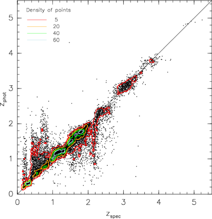
Figure 1.— Contour plot of quasar photometric redshifts assigned by the instance-based learner versus spectroscopic redshifts for the SDSS DR5 pseudo-blind testing sample of 11,149 of 55,746 quasars described in the text. For contouring, the objects are placed in bins of 0.05 in redshift, although the values on both axes are continuous. The variance between the two measures over the whole redshift range is $0.123\pm 0.002$. Compared to Figure 3, there are no regions of ‘catastrophic’ failure, in which objects are assigned a very different redshift to the true value, just a smoothly declining spread of outliers. There are no objects outside the range of redshifts plotted.

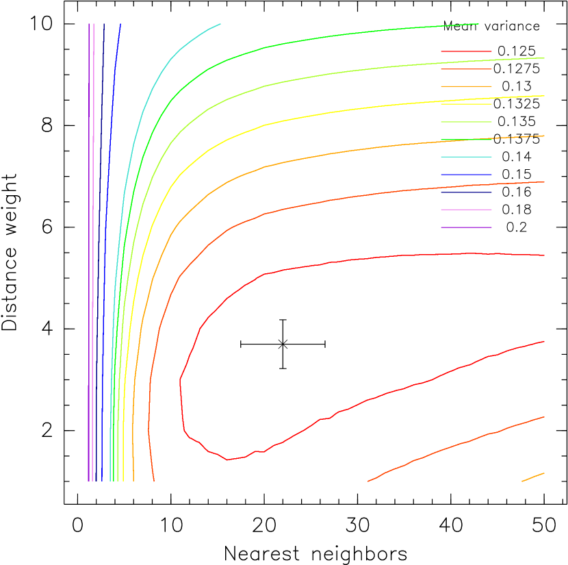
Figure 2.— Effect of varying the number of nearest neighbors and the distance weighting of the instance-based learner for the pseudo-blind test on the SDSS DR5 dataset, showing the mean from ten different training to pseudo-blind test splits of the data with a varying random seed. The model which gives the lowest variance is marked with $1\sigma$ error bars.

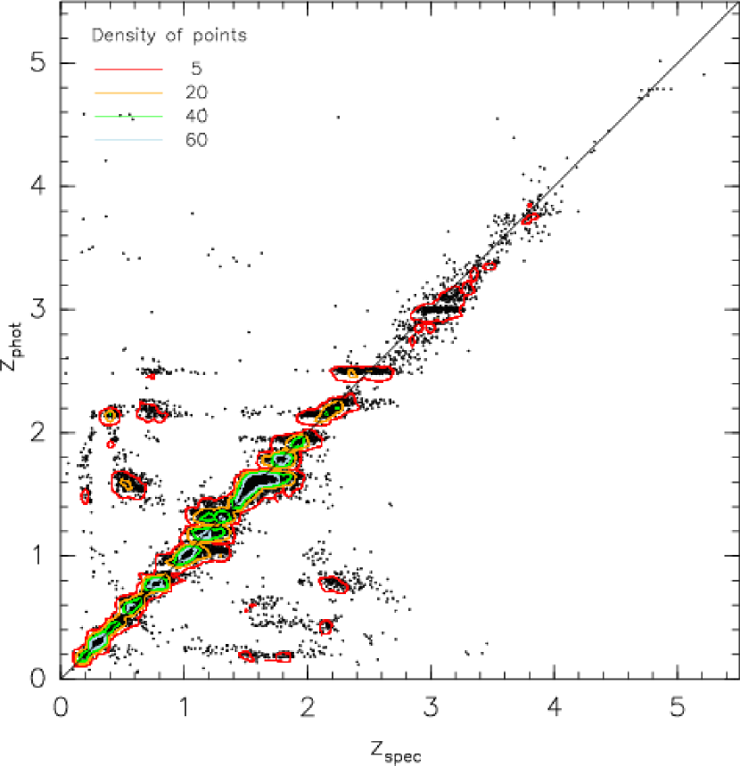
Figure 3.— As Figure 1, but showing the results for the CZR photozs. The regions of catastrophic failure are seen, and the overall variance is $\sigma^{2}=0.265\pm 0.006$. The values of $z_{\mathrm{phot}}$ resulting from this method are in bins of width 0.05. Here, a uniformly distributed random offset up to $\pm 0.025$ has been added to the values of $z_{\mathrm{phot}}$ for clarity.

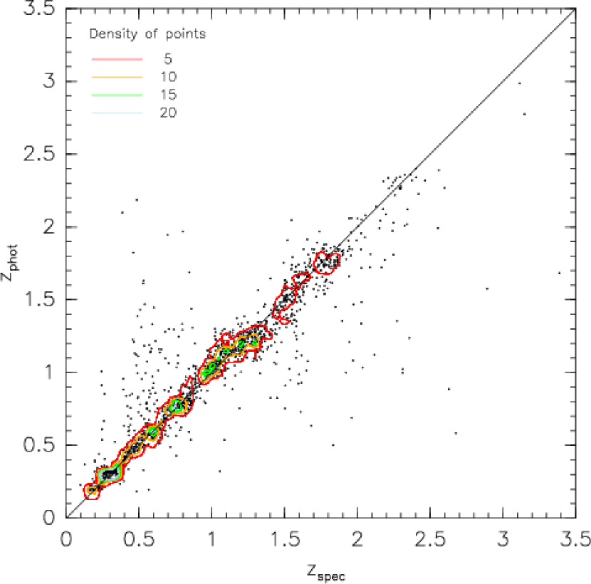
Figure 4.— As Figure 1, but showing the results for 1,528 of 7,642 quasars present in the SDSS DR5 cross-matched to the GALEX GR2. The variance is improved to $\sigma^{2}=0.054\pm 0.005$.

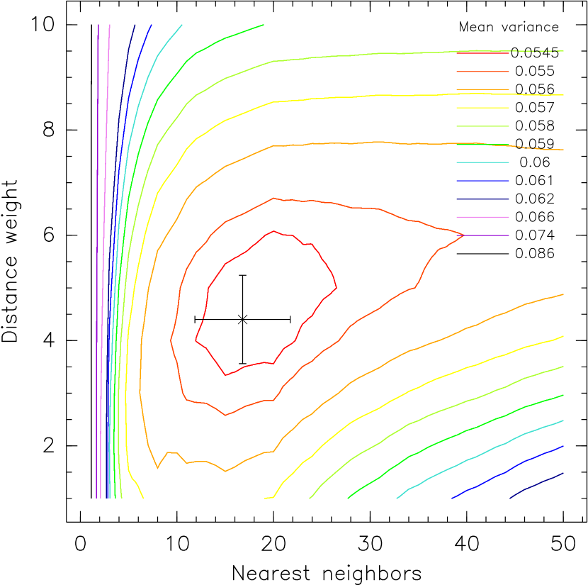
Figure 5.— As Figure 2, but for the SDSS+GALEX dataset shown in Figure 4.

Table 1Summary of photometric redshift samples described in this paper.

Dataset	Method	Variance	Variance/(1+z)	Mean $\Delta z/(1+z)$	$\%\Delta z<0.1$	$\%\Delta z<0.2$	$\%\Delta z<0.3$
SDSS	IB	$0.123\pm 0.002$	$0.034\pm 0.001$	$0.095\pm 0.001$	$54.9\pm 0.7$	$73.3\pm 0.6$	$80.7\pm 0.3$
SDSS+GALEX	IB	$0.054\pm 0.005$	$0.014\pm 0.002$	$0.060\pm 0.003$	$70.8\pm 1.2$	$85.8\pm 1.0$	$90.8\pm 0.7$
GALEX-SDSS-only	IB	$0.090\pm 0.007$	$0.022\pm 0.001$	$0.081\pm 0.003$	$62.0\pm 1.4$	$78.9\pm 1.0$	$85.2\pm 1.2$
SDSS	CZR	$0.265\pm 0.006$	$0.079\pm 0.003$	$0.115\pm 0.002$	$63.9\pm 0.3$	$80.2\pm 0.4$	$85.7\pm 0.3$
SDSS+GALEX	CZR	$0.136\pm 0.015$	$0.031\pm 0.006$	$0.071\pm 0.005$	$74.9\pm 1.4$	$86.9\pm 0.6$	$91.0\pm 0.8$
GALEX-SDSS-only	CZR	$0.158\pm 0.013$	$0.041\pm 0.004$	$0.081\pm 0.004$	$74.1\pm 0.8$	$86.2\pm 0.7$	$89.7\pm 0.6$

References

- Abazajian et al. (2004) Abazajian, K. et al. 2004, AJ, 128, 502
- Aha et al. (1991) Aha, D. W., Kibler, D., & Albert, M. K. 1991, Machine Learning, 6, 37
- Babbedge et al. (2004) Babbedge, T. S. R. et al. 2004, MNRAS, 353, 279
- Ball et al. (2006) Ball, N. M., Brunner, R. J., Myers, A. D., & Tcheng, D. 2006, ApJ, 650, 497
- Ball et al. (2004) Ball, N. M., Loveday, J., Fukugita, M., Nakamura, O., Okamura, S., Brinkmann, J., & Brunner, R. J. 2004, MNRAS, 348, 1038
- Baum (1962) Baum, W. A. 1962, in IAU Symp. 15: Problems of Extra-Galactic Research, 390
- Beckwith et al. (2006) Beckwith, S. V. W. et al. 2006, AJ, 132, 1729
- Benítez (2000) Benítez, N. 2000, ApJ, 536, 571
- Brunner et al. (1997) Brunner, R. J., Connolly, A. J., Szalay, A. S., & Bershady, M. A. 1997, ApJ, 482, L21
- Brunner et al. (2000) Brunner, R. J., Szalay, A. S., & Connolly, A. J. 2000, ApJ, 541, 527
- Budavári et al. (2001) Budavári, T. et al. 2001, AJ, 122, 1163
- Cannon et al. (2006) Cannon, R. et al. 2006, MNRAS, 372, 425
- Cardelli et al. (1989) Cardelli, J. A., Clayton, G. C., & Mathis, J. S. 1989, ApJ, 345, 245
- Coe et al. (2006) Coe, D., Benítez, N., Sánchez, S. F., Jee, M., Bouwens, R., & Ford, H. 2006, AJ, 132, 926
- Collister et al. (2007) Collister, A. et al. 2007, MNRAS, 375, 68
- Collister & Lahav (2004) Collister, A. A. & Lahav, O. 2004, PASP, 116, 345
- Connolly et al. (1998) Connolly, A. J., Szalay, A. S., & Brunner, R. J. 1998, ApJ, 499, L125
- Cover & Hart (1967) Cover, T. M. & Hart, P. E. 1967, IEEE Transactions on Information Theory, 13, 21
- Croom et al. (2004) Croom, S. M., Smith, R. J., Boyle, B. J., Shanks, T., Miller, L., Outram, P. J., & Loaring, N. S. 2004, MNRAS, 349, 1397
- Csabai et al. (2003) Csabai, I. et al. 2003, AJ, 125, 580
- Eisenstein et al. (2001) Eisenstein, D. J. et al. 2001, AJ, 122, 2267
- Firth et al. (2003) Firth, A. E., Lahav, O., & Somerville, R. S. 2003, MNRAS, 339, 1195
- Goldberg (1989) Goldberg, D. E. 1989, Genetic Algorithms in Search, Optimization, and Machine Learning (Reading, MA: Addison-Wesley)
- Goldberg (2002) Goldberg, D. E. 2002, Design of innovation: Lessons from and for competent genetic algorithms (Boston, MA: Kluwer Academic Publishers)
- Gwyn & Hartwick (1996) Gwyn, S. D. J. & Hartwick, F. D. A. 1996, ApJ, 468, L77
- Hastie et al. (2001) Hastie, T., Tibshirani, R., & Friedman, J. 2001, The Elements of Statistical Learning (Springer)
- Haupt & Haupt (1998) Haupt, R. L. & Haupt, S. E. 1998, Practical Genetic Algorithms (New York: Wiley Inter-Science)
- Hogg et al. (1998) Hogg, D. W. et al. 1998, AJ, 115, 1418
- Holland (1975) Holland, J. H. 1975, Adaptation in Natural and Artificial Systems: An Introductory Analysis with Applications to Biology, Control and Artificial Intelligence (Ann Arbor, MI: The University of Michigan Press)
- Koo (1985) Koo, D. C. 1985, AJ, 90, 418
- Lanzetta et al. (1996) Lanzetta, K. M., Yahil, A., & Fernandez-Soto, A. 1996, Nature, 381, 759
- Lawrence et al. (2006) Lawrence, A. et al. 2006, preprint, astro-ph/0604426
- Loh & Spillar (1986) Loh, E. D. & Spillar, E. J. 1986, ApJ, 303, 154
- Martin et al. (2005) Martin, D. C. et al. 2005, ApJ, 619, L1
- Mobasher et al. (1996) Mobasher, B., Rowan-Robinson, M., Georgakakis, A., & Eaton, N. 1996, MNRAS, 282, L7
- Myers et al. (2007a) Myers, A. D., Brunner, R. J., Nichol, R. C., Richards, G. T., Schneider, D. P., & Bahcall, N. A. 2007a, ApJ, in press (astro-ph/0612190)
- Myers et al. (2007b) Myers, A. D., Brunner, R. J., Richards, G. T., Nichol, R. C., Schneider, D. P., & Bahcall, N. A. 2007b, ApJ, in press, (astro-ph/0612191)
- Myers et al. (2006) Myers, A. D. et al. 2006, ApJ, 638, 622
- Padmanabhan et al. (2005) Padmanabhan, N. et al. 2005, MNRAS, 359, 237
- Richards et al. (2001) Richards, G. T. et al. 2001, AJ, 122, 1151
- Sawicki et al. (1997) Sawicki, M. J., Lin, H., & Yee, H. K. C. 1997, AJ, 113, 1
- Schlegel et al. (1998) Schlegel, D. J., Finkbeiner, D. P., & Davis, M. 1998, ApJ, 500, 525
- Skrutskie et al. (2006) Skrutskie, M. F. et al. 2006, AJ, 131, 1163
- Stoughton et al. (2002) Stoughton, C. et al. 2002, AJ, 123, 485
- Tagliaferri et al. (2002) Tagliaferri, R., Longo, G., Andreon, S., Capozziello, S., Donalek, C., & Giordanoet, G. 2002, preprint, astro-ph/0203445
- Vanden Berk et al. (2005) Vanden Berk, D. E. et al. 2005, AJ, 129, 2047
- Vanzella et al. (2004) Vanzella, E. et al. 2004, A&A, 423, 761
- Wadadekar (2005) Wadadekar, Y. 2005, PASP, 117, 79
- Wang et al. (1998) Wang, Y., Bahcall, N., & Turner, E. L. 1998, AJ, 116, 2081
- Way & Srivastava (2006) Way, M. J. & Srivastava, A. N. 2006, ApJ, 647, 102
- Weinstein et al. (2004) Weinstein, M. A. et al. 2004, ApJS, 155, 243
- Welge et al. (1999) Welge, M., Hsu, W. H., Auvil, L. S., Redman, T. M., & Tcheng, D. 1999, in 12th National Conference on High Performance Networking and Computing (SC99)
- Werner et al. (2004) Werner, M. W. et al. 2004, ApJS, 154, 1
- Williams et al. (1996) Williams, R. E. et al. 1996, AJ, 112, 1335
- Williams et al. (2000) —. 2000, AJ, 120, 2735
- Witten & Frank (2000) Witten, I. H. & Frank, E. 2000, Data Mining (Morgan Kaufmann)
- Wolf et al. (2003) Wolf, C., Wisotzki, L., Borch, A., Dye, S., Kleinheinrich, M., & Meisenheimer, K. 2003, A&A, 408, 499
- Wolf et al. (2004) Wolf, C. et al. 2004, A&A, 421, 913
- Wu et al. (2004) Wu, X.-B., Zhang, W., & Zhou, X. 2004, Chinese Journal of Astronomy and Astrophysics, 4, 17
- York et al. (2000) York, D. G. et al. 2000, AJ, 120, 1579