New measurements of cosmic infrared background fluctuations from early epochs.

Abstract

Cosmic infrared background fluctuations may contain measurable contribution from objects inaccessible to current telescopic studies, such as the first stars and other luminous objects in the first Gyr of the Universe’s evolution. In an attempt to uncover this contribution we have analyzed the GOODS data obtained with the Spitzer IRAC instrument, which are deeper and cover larger scales than the Spitzer data we have previously analyzed. Here we report these new measurements of the cosmic infrared background (CIB) fluctuations remaining after removing cosmic sources to fainter levels than before. The remaining anisotropies on scales $\sim\!0.5^{\prime}\!-\!10^{\prime}$ have a significant clustering component with a low shot-noise contribution. We show that these fluctuations cannot be accounted for by instrumental effects, nor by the Solar system and Galactic foreground emissions and must arise from extragalactic sources.

1 Introduction

Cosmic infrared background (CIB) contains emissions from all luminous including those inaccessible to current telescopic studies (see Kashlinsky 2005 for recent review). If the first stars (commonly called Population III) were massive Abell (2002); Bromm et al (1999); Bromm & Larson (2004), they could produce significant levels of the CIB with measurable fluctuations Santos et al (2002); Salvaterra & Ferrara (2003); Kashlinsky et al (2004); Cooray et al (2004); Madau & Silk (2005); Fernandez & Komatsu (2006). Recently, in an attempt to uncover these signatures of early stars, we have detected significant CIB fluctuations after removing galaxies to faint limits in deep Spitzer data (Kashlinsky et al 2005; hereafter KAMM). The measured fluctuations cannot arise from the Solar System and Galactic foreground emissions, or from the remaining galaxies and must come from early extragalactic sources, particularly the first stars. To solidify these findings we have now analyzed deeper datasets from the GOODS survey Dickinson et al (2003) covering different and larger areas of the sky and with observing procedures which allow us to test for a wide range of systematic errors in the data.

In this Letter we present the new measurements using the GOODS Spitzer/IRAC data at 3.6, 4.5, 5.8 and 8 $\mu$m. At the magnitude limit of the QSO1700 data we measure a similar CIB signal consistent with its cosmological origin. After removing still fainter sources, we find that the bulk of the CIB fluctuations remain out to $\sim$10^′, the limit of our fields. This shows that the signal originates in populations significantly fainter than our cutoff. We also test for possible systematic errors in the fluctuations by cross-correlating the data for the same regions taken at different epochs and in different detector orientations, showing only a small contribution from the instrument systematics. The Galactic and zodiacal foregrounds are generally also small, although as in the QSO1700 data, we find a possibility of a significant cirrus pollution of the Channel 4 fluctuations. Cosmological interpretation of the results is given in a separate paper (Kashlinsky, Arendt, Mather & Moseley 2006).

2 Data processing

Table 1 shows parameters of the data used in this and earlier (KAMM) analyses. The new data from the GOODS Spitzer Legacy Program(PID=194, pipeline version=S11.4.0, except S11.0.2 for CDFS Epoch 1, Dickinson et al 2003) come from measurements in two parts of the sky, HDFN in the North and CDFS in the South, observed at two different Epochs, E1 and E2, $\sim$6 months apart. The two epochs had different detector orientations rotated by $\sim$180^∘ with respect to the sky, allowing a test for certain instrumental effects and zodiacal light. The final mosaics were assembled from the individual Basic Calibrated Data (BCD) frames which were self-calibrated using the method of Fixsen et al (2000) similarly to KAMM; no extended source calibration factors were applied to the data. To evaluate the random noise level of the maps, alternate calibrated frames for each dataset were mapped into separate “A” and “B” mosaics.

The assembled maps were cleaned of resolved sources in two steps: First, an iterative procedure was applied which computes the standard deviation, $\sigma$, of the image, and masks pixels exceeding $N_{\rm cut}\sigma$ along with $N_{\rm mask}\!\times\!N_{\rm mask}$ surrounding pixels until no pixels exceed $N_{\rm cut}\sigma$. We adopted $N_{\rm mask}$=3 and $N_{\rm cut}$=4, when enough pixels ($\geq$65%) remain for robust Fourier analysis. Second, similar to KAMM, we subtracted the Model of the individual sources using a variant of the CLEAN algorithm H$\ddot{\rm o}$gbom (1974). In a normal CLEAN procedure, the clean components are convolved with an idealized clean beam to produce a map without sidelobe artifacts; we stop short of this, working with the residual map from which the dirty beam and its artifacts have been removed. We construct the Model from the original unmasked mosaics for each channel as follows: (1) the maximum pixel intensity is located, (2) the PSF is then scaled to half of this intensity and subtracted from the image, (3) the process is iterated, saving intermediate results.

Because spectroscopic redshifts are unavailable and resolving individual sources is difficult in the confusion limit of these observations, we removed the sources via the Model to a fixed level of the shot noise. Its amplitude due to remaining sources is $P_{\rm SN}=\int_{m_{\rm lim}}^{\infty}[S(m)]^{2}dN/dm\;dm$. $S(m)$ is the flux of magnitude $m$ in nW/m²; diffuse flux is defined as $\nu I_{\nu}$, with $I_{\nu}$ being the surface brightness in MJy/sr. With the Model iteration where the maps remain close to a fixed $P_{\rm SN}$ we can probe the CIB fluctuations produced by populations below a relatively well-defined flux threshold. In principle, the remaining instrument noise, truncated of its high positive peaks, may have an imprint of the beam and mimic part (or even most) of the shot noise from cosmic sources. In that case, the shot noise we present in Fig. 1 represents an upper limit on the contribution from cosmic sources making our conclusions below stronger.

The maps, clipped and with the Model subtracted, were Fourier-transformed and subjected to all the same tests as in KAMM; the additional tests possible with this data are described below. The fluctuation field, $\delta F($$x$), was not weighted for the results presented here (although we checked that weighting by the observation time in each pixel does not lead to any appreciable changes), and its Fourier transform, $f($$q$$)=\int\delta F($$x$$)\exp(-i$$x$$\cdot$$q$$)d^{2}x$ was calculated using the fast Fourier transform. The 2-D power spectrum is defined as $P_{2}(q)\equiv\langle|f_{q}|^{2}\rangle$ and in this definition a typical flux fluctuation is $\simeq\sqrt{q^{2}P_{2}(q)/2\pi}$ on the angular scale of wavelength $2\pi/q$. The blanked pixels were assigned $\delta F$=0, thereby not adding power to the eventual power spectrum. Muxbleed was removed by zeroing the corresponding frequencies in the $(u,v)$ plane before computing the power spectrum of the maps, $P_{S}$. We subtracted remaining linear gradients from the maps before clipping and again after clipping. The noise power spectrum, $P_{N}$, was evaluated from the $\frac{1}{2}(A-B)$ data using the mask from the main maps. The remaining power spectrum was evaluated as $P=P_{S}-P_{N}$.

3 Results

Fig. 1 shows results from the new data compared to the earlier QSO1700 data analysis. As discussed above, in the present analysis we can regulate the faint source removal from the maps by fixing the floor level of the shot noise, whose amplitude $P_{\rm SN}$ was evaluated from the fits to the small scale power spectrum using our model for the beam. Because we mapped the GOODS data onto 1.2^′′ pixels (instead of $0.6^{\prime\prime}$ for the QSO1700 data) the beam used for generating the Model was a slightly smoothed version of that used in the QSO1700 data.

The upper panels in the figure show the CIB fluctuations in the GOODS fields evaluated at the Model iteration when $P_{\rm SN}$ roughly corresponds to that in the earlier QSO1700 analysis. The figure shows CIB fluctuations consistent with those in the earlier analyzed QSO1700 dataset. Our results are consistent that at the same level of $P_{\rm SN}$ all data are probing the same populations. (At the deeper Model iterations extra galaxy populations were removed in the present analysis compared to the QSO1700 field and at shallower Model iterations extra galaxy populations were removed in the QSO1700 field). Because of longer integration in the new data, we can remove sources to still lower $P_{\rm SN}$. The lower panels of Fig. 1 show the CIB fluctuations remaining in the maps at the lowest common value of $P_{\rm SN}$; the signal shown here comes from still fainter sources than the limits in the earlier KAMM analysis.

4 Discussion

The following can, in principle, contribute to the detected fluctuations 1) instrumental (systematic and random), 2) source artefacts, 3) Solar System and Galactic foregrounds, and 4) extragactic sources. We briefly discuss the contributions of each and conclude that (with the possible exception of the 8$\mu$m data) the detected fluctuations are due to CIB from extragalactic sources below our removal threshold set by the shot-noise amplitude.

Checking for systematics: E1 vs E2. In measuring the faint, low spatial frequency backgrounds, control of systematic errors remains a major challenge. Of particular concern is scattered light in the Spitzer and IRAC optical systems, which can spread the light from point sources over large spatial scales. Some scattered light retains a fixed relative position with respect to the originating point source. Other scattered light gets to the focal plane after multiple reflections, and its spacing with respect to the originating source will vary as the source is moved in the field of view. Finally, some scattered light may arise from sources outside the field of view, and may change its illumination of the detector in a complex way as the telescope is moved on the sky. Given that scattered light and detector artifacts can cause structure in the image, it is important that we use observations for these studies which allow us to evaluate the size of such possible effects in the images we analyze.

To search for instrumental sources of large scale power, we used the partially overlapping E1 and E2 data of the HDN and CDFS regions in which the telescope and optical system are rotated by $\sim$180 degrees with respect to the field of view. Using such observations, we can compare the source-removed sky maps from the two epochs to separate structure which is unchanged in inertial coordinates, and thus presumably arising from the sky, and that which changes, which could represent an instrumental contribution.

We selected overlapping subfields for the final mosaicked images which had fairly homogeneous exposures. The latter limited the selected areas to approximately the same size: $142\times 504$ arcsec in the CDFS field and $149\times 504$ arcsec in the HDFN area. We then computed the subfield and cross-subfield correlation functions and coefficients to verify that the signal is the same at each Epoch and is detector-orientation independent. Having carried out the point source subtraction and gradient removal on the two epochs, we compared the correlation function of the difference map to that of each of the individual maps, and also did a cross correlation analysis. In both cases, we find that all of the large scale power arises from the sky down to the presented statistical error bars; this rules out any significant contribution from instrumental scattered light and detector artifacts.

We also estimated that there is at most only a small contribution to the measured power spectrum from image artefacts, such as e.g. associated with occasional strong muxbleed. This was done by selecting sub-regions excluding the areas of obvious artefacts. (This is responsible for a slight excess in power at 3.6 $\mu$m around 1-2 arcmin for one of the fields).

Procedural sources of large-scale power. Because IRAC’s calibration does not include zero-flux closed-shutter data, a degeneracy remains in the absolute zero point of the solution. A similar degeneracy is present with respect to first-order gradients in the mosaics. However higher-order gradients are not degenerate. Because of these degeneracies, linear gradients have been fit and subtracted from the self-calibrated mosaicked images. The zero-level is unimportant to this study, so all analyzed maps are set to a mean intensity equal to zero.

We find - via simulations - that in small, but non-negligible number of cases the gradient-subtraction can also remove the genuine cosmic power at the largest scales and the power shown there should thus be treated as the lower limit on any cosmic fluctuations. However, we find in the QSO1700, the HDFN-E1 and HDFN-E2 analyses that the results do not change appreciably even if the extra-subtraction is done at each step of the Model iteration. The CDFS fields, which have a common overlap at both Epochs, exhibit more sensitivity (at the level of $\sim 20\%$ in the largest bins) to this extra gradient subtraction. Taken together this is consistent with the cosmic nature of the fluctuations shown in Fig. 1 and the CDFS field happening to be statistically more sensitive to the extra gradient subtraction.

The possible contributions from incompletely removed galaxies are also small as discussed in KAMM. Briefly: 1) the measured fluctuations are independent of the masking and clipping parameters. E.g. when clipping is $N_{\rm cut}$=2 only 6% of the maps remained KAMM , but the correlation function, which replaces the power spectrum as a measure of large-scale correlations for such deeply cut maps, remained practically the same. 2) The results are invariant when the masking size around each clipped pixel is increased (from $N_{\rm mask}$=3 to 7). This mask is larger than the typical galaxy size at $z{{}_{>}\atop{}^{\sim}}$0.1 so individual galaxies are expected to have been removed completely. The Model further removes much of the remaining emissions at larger angles. 3) We measure the clustering component from $\sim 0.5^{\prime}$ to $\sim$5-10^′, which subtend 1 to 10 Mpc at $z$=0.1,1. If the power comes from the incompletely removed local galaxies, its angular spectrum should reflect the slope of the observed galaxy two-point correlation function, contrary to Fig. 1. 4) The results are the same for all fields at the fixed level of shot-noise. The level of the remaining $P_{\rm SN}$ fixes the amount of the remaining flux from incompletely removed sources of full magnitude $m$. The contribution from them to the large scale clustering should then have been a proportional fraction of the CIB clustering produced by the parental sources. 5) By construction in their results, KAMM identified the appropriate Model iteration number where the clean components become largely uncorrelated with the sources in the original image. (Here we use $P_{\rm SN}$ as the alternative criterion).

Zodiacal and Galactic foregrounds. The cirrus flux in Table 1 are the SPOT estimates of ISM intensity, based on the Schlegel et al (1998) 100 $\mu$m IRAS intensity and temperature maps and a spectral scaling relation derived from DIRBE, ISO and AROME observations of the ISM (http://ssc.spitzer.caltech.edu/documents/background/bgdoc_release.html; Reach & Boulanger 1997). Fluctuations in the cirrus emission are assumed to be at the 1% level as suggested by the intensity of the fluctuation spectrum of a low galactic latitude field in which cirrus emission was clearly evident at 8 $\mu$m (KAMM). As in the QSO1700 data, the cirrus may contribute a non-negligible contribution at 8 $\mu$m, and prevents us from isolating the cosmological signal there. Even assuming that the entire signal at 8 $\mu$m is produced by cirrus and taking the mean Galactic cirrus energy distribution Arendt et al (1998) gives an upper limit on the cirrus emission at shorter wavelengths well below the signal we detect.

The range in zodiacal light intensity in the time spanned by the observations is shown in Table 1. Its fluctuations are a factor of $\simeq$4-15 below those from cirrus. A limit of $\delta F<$0.1 $\rm nW/m^{2}/sr\$at 8 $\mu$m due to zodiacal light was derived by KAMM from the observed dispersion of the data at two epochs separated by about six months. This limit at 8 $\mu$m (with relative fluctuations at a much lower level than the $<$0.2% limit by Abraham et al. (1997) at 25 $\mu$m) was then scaled to the shorter wavelengths using the zodiacal light spectrum derived from COBE/DIRBE data (Kelsall et al. 1998). In the present study too we find no evidence for zodiacal emission above the instrument noise levels; the arcminute limits on zodiacal fluctuations from subtracting the two Epochs are $\delta F{{}_{<}\atop{}^{\sim}}$0.05 $\rm nW/m^{2}/sr\$at 8 $\mu$m.

Extragalactic sources. The detected signal is thus due to CIB fluctuations from extragalactic sources, such as ordinary galaxies and the putative Population III. KAMM estimated that the CIB flux from the remaining galaxies was only $\simeq$0.15 $\rm nW/m^{2}/sr\$so that they were unlikely to account for the strong clustering signal. The present data enable us to eliminate intervening sources down to lower levels of the shot noise, or lower flux limits. The detected signal has to originate in still fainter sources. In a companion paper (Kashlinsky, Arendt, Mather & Moseley 2006) we discuss the constraints our results (both the shot-noise and clustering components of the fluctuations) place on the nature of the sources contributing them. We show that the signal at 3.6, 4.5 $\mu$m must arise from very faint populations with individual fluxes ${{}_{<}\atop{}^{\sim}}$10-20 nJy and that the amplitude of the fluctuations at arcminute scales requires these populations to be significantly more luminous per unit mass than the present-day ones.

This work is supported by NSF AST-0406587 and NASA Spitzer NM0710076 grants.

Table 1: Analyzed Fields

Parameter	Channel	QSO1700	HDFN-E	HDFN-E2	CDFS-E1	CDFS-E2
($l_{\rm Gal},b_{\rm Gal}$) (deg)	$\cdots$	($94.4,36.1$)	($125.9,54.8$)	($125.9,54.8$)	($223.6,-54.4$)	($223.6,-54.4$)
($\lambda_{\rm Ecl},\beta_{\rm Ecl}$) (deg)	$\cdots$	($194.3,83.5$)	($148.4,57.3$)	($148.4,57.3$)	($41.1,-45.2$)	($41.1,-45.2$)
Size (arcmin)	$\cdots$	$5.1\!\times\!11.5$	$10.2\!\times\!10.2$	$10.2\!\times\!10.2$	$8.8\!\times\!8.4$	$9.0\!\times\!8.4$
$\langle t_{\rm obs}\rangle$ (hr)	$\cdots$	7.8	20.9	20.7	23.7	22.4
$P_{\rm SN}$ $({\rm nW}2{\rm m}^{-4}{\rm sr})$	1 (3.6 $\micron$)	$5.8\!\times\!10^{-11}$	$1.9\!\times\!10^{-11}$	$1.9\!\times\!10^{-11}$	$2.2\!\times\!10^{-11}$	$2.3\!\times\!10^{-11}$
Flux: zodi (nW/m2/sr)	1 (3.6 $\micron$)	32	45–47	37–38	48–51	48–49
Flux: cirrus (nW/m2/sr)	1 (3.6 $\micron$)	2.5	0.8	0.8	0.8	0.8
$P_{\rm SN}$ $({\rm nW}2{\rm m}^{-4}{\rm sr})$	2 (4.5 $\micron$)	$6.0\!\times\!10^{-11}$	$1.1\!\times\!10^{-11}$	$1.0\!\times\!10^{-11}$	$9.5\!\times\!10^{-12}$	$1.1\!\times\!10^{-11}$
Flux: zodi (nW/m2/sr)	2 (4.5 $\micron$)	132	174–185	146–153	189–204	165–176
Flux: cirrus (nW/m2/sr)	2 (4.5 $\micron$)	2.7	1.3	1.3	1	1
$P_{\rm SN}$ $({\rm nW}2{\rm m}^{-4}{\rm sr})$	3 (5.8 $\micron$)	$6.0\!\times\!10^{-10}$	$1.2\!\times\!10^{-10}$	$1.3\!\times\!10^{-10}$	$1.5\!\times\!10^{-10}$	$1.5\!\times\!10^{-10}$
Flux: zodi (nW/m2/sr)	3 (5.8 $\micron$)	873	1192–1250	996–1026	1256–1327	1179–1243
Flux: cirrus (nW/m2/sr)	3 (5.8 $\micron$)	7.8	36.	3.6	2.6	2.6
$P_{\rm SN}$ $({\rm nW}2{\rm m}^{-4}{\rm sr})$	4 (8 $\micron$)	$4.4\!\times\!10^{-10}$	$1.0\!\times\!10^{-10}$	$1.1\!\times\!10^{-10}$	$1.1\!\times\!10^{-10}$	$1.4\!\times\!10^{-10}$
Flux: zodi (nW/m2/sr)	4 (8 $\micron$)	1723	2411–2500	2012–2054	2509–2614	2454–2562
Flux: cirrus (nW/m2/sr)	4 (8 $\micron$)	33.8	16.1	16.1	10.1	10.1

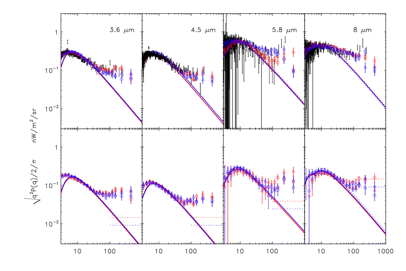
Figure 1: CIB fluctuations from the analyzed fields. The fluctuation spectrum was evaluated by averaging over the concentric rings center at given $q$ and the errors shown correspond to the cosmic variance for the estimates, i.e. the Poissonian errors of relative amplitude $N_{q}^{-1/2}$ with $N_{q}$ being the number of independent Fourier elements used in determining the power at $q$. Top: the CIB fluctuations were evaluated for the shot-noise levels approximately corresponding to the $P_{\rm SN}$ of the QSO1700 data. Black error bars show the QSO1700 fields results from KAMM . Red symbols correspond to the HDFN fields and blue symbols denote the CDFS data results. Triangles correspond to E1 and circles to E2. The lines show the fluctuations due to shot-noise from the remaining sources. Bottom: Same as top shown for the lowest levels of $P_{\rm SN}$ reached with the new data. The blue and red dotted lines show the estimated cirrus fluctuations for the CDFS and HDFN fields respectively.

References

- Abell (2002) Abell, T. 2002, Science, 295, 93
- Ábrahám et al (1997) Ábrahám, P., Leinert, Ch., & Lemke, D. 1997, A&A, 328, 702
- Arendt et al (1998) Arendt, R. et al 1998, Ap.J., 508,74
- Bromm et al (1999) Bromm, V. et al 1999, Ap.J., 527, L5
- Bromm & Larson (2004) Bromm, V. & Larson, R. 2004, Ann. Rev. A. A., 42, 79
- Cooray et al (2004) Cooray, A. et al 2004, Ap.J., 606, 611
- Dickinson et al (2003) Dickinson, M. et al 2003, “The great observatories origins deeps survey”, in “The mass of galaxies at low and high redshift”, ed. R. Bender & A. Renzini, astro-ph/0204213
- Fernandez & Komatsu (2006) Fernandez, E. R. & Komatsu, E. 2005, Ap.J., 646, 703
- Fixsen et al (2000) Fixsen, D. J., Moseley, S. H. & Arendt, R. G. 2000, Ap. J. Suppl., 128, 651
- Hgbom (1974) Hgbom, J. 1974, Ap.J.Suppl., 15,417
- Kashlinsky (2005) Kashlinsky, A. 2005, Phys. Rep., 409, 361-438
- Kashlinsky et al (2004) Kashlinsky, A., Arendt, R., Gardner, J.P., Mather, J.C., & Moseley, S.H. 2004, Ap.J., 608, 1
- (13) Kashlinsky, A., Arendt, R., Mather, J.C. & Moseley, S.H. 2005, Nature, 438, 45
- Kashlinsky et al (2006) Kashlinsky, A., Arendt, R., Mather, J.C. & Moseley, S.H. 2006, Ap.J., submitted.
- Kelsall et al (1998) Kelsall, T. et al 1998, Ap.J., 508, 44
- Madau & Silk (2005) Madau, P. & Silk, J. 2005,MNRAS, 359, L37
- Reach & Boulagger (1997) Reach, W. T. & Boulanger, F. 1997, in “Infrared emission from interstellar dust in the local interstellar medium: The Local Bubble and Beyond”, eds. D. Breitschwerdt, M. J. Freyburg, & J. Trumper;352-362, Springer:Berlin
- Santos et al (2002) Santos, M.R., Bromm, V., Kamionkowski, M. 2002,MNRAS,336,1082
- Salvaterra & Ferrara (2003) Salvaterra, R. & Ferrara, A. 2003, MNRAS, 339, 973
- Schlegel et al (1998) Schlegel, D., Finkbeiner, D. & Davis, M. 1998, Ap.J., 500, 525