PHOTOSPHERIC MAGNETIC FIELD OF THE SUN: TWO PATTERNS OF THE LONGITUDINAL DISTRIBUTION

Abstract

Longitudinal distributions of the photospheric magnetic field studied on the basis of National Solar Observatory (Kitt Peak) data (1976 – 2003) displayed two opposite patterns during different parts of the 11-year solar cycle. Heliolongitudinal distributions differed for the ascending phase and the maximum of the solar cycle on the one hand, and for the descending phase and the minimum on the other, depicting maxima around two diametrically opposite Carrington longitudes ($180^{\circ}$ and $0^{\circ}/360^{\circ}$). Thus the maximum of the distribution shifted its position by $180^{\circ}$ with the transition from one characteristic period to the other. Two characteristic periods correspond to different situations occurring in the 22-year magnetic cycle of the Sun, in the course of which both the global magnetic field and the magnetic field of the leading sunspot in a group change their sign. During the ascending phase and the maximum (active longitude $180^{\circ}$) polarities of the global magnetic field and those of the leading sunspots coincide, whereas for the descending phase and the minimum (active longitude $0^{\circ}/360^{\circ}$) the polarities are opposite. Thus the observed change of active longitudes may be connected with the polarity changes of Sun’s magnetic field in the course of 22-year magnetic cycle.

1 Introduction

The 11-year cycle of solar activity reflects the cyclic behavior of the Sun’s large-scale magnetic field. In the course of this cycle not only do the number and intensity of various activity manifestations experience systematic changes but so does their distribution over the solar surface . In contrast to the well-established features of the latitudinal distribution of the solar activity, seen for example in butterfly diagrams, there exists a variety of evidence on the longitudinal distribution that is difficult to reconcile in one unified picture.

The literature concerned with the problem of active longitudes is too vast to give a detailed review here; we refer, therefore, to the review article by Gaizauskas (1993) and also to Bai (2003), Bigazzi and Ruzmaikin (2004), and references therein. Some references concerning this problem are also given in one of our papers (Vernova et al., 2004). Here we shall confine ourselves to some of the principal questions arising in the study of the active longitudes.

An important problem is the stability and lifetime of the active longitudes, which vary over a wide range in different studies. Some authors have found active longitudes existing from several successive solar rotations (Bumba and Howard, 1965; de Toma, White, and Harvey, 2000) to 20 – 40 consecutive rotations (Bumba and Howard, 1969). Yet according to Balthasar and Schüssler (1983) there is a ”solar memory” for preferred longitudes of activity extending at least over one, and probably two cycles. Active zones persisting for three solar cycles were described in Bai (1988) and Jetsu et al. (1997).

Another important problem is the localization of active longitudes relative to the Carrington framework. Some authors observed that the longitudes at which sunspots preferentially occur, do not display differential rotation: The active longitudes experience more rigid rotation with the Carrington period (T = 27.2753 days) approximately. So, Bumba and Howard (1969) state that subsurface sources that produce active longitudes rotate with the synodic period regardless of the region latitude. Complexes of activity described in Gaizauskas et al. (1983) were found to rotate at a steady rate, sometimes coinciding with the Carrington rate and sometimes slower or faster. The tendency of the activity of two successive solar cycles to appear at the same preferred longitudes was found in Benevolenskaya et al. (1999) and Bumba, Garcia, and Klvan̆a (2000).

In some investigations constant rotation rate of active longitudes with a period differing from the Carrington period was registered. Two main periodicities (22.07 and 26.72 days) were detected in the major solar flare data (Jetsu et al., 1997). Moreover, in some cases the rotation rate changed from cycle to cycle and even during an individual solar cycle; see, e.g., Bogart (1982).

In contrast these results favoring the rigid rotation of active longitudes, Berdyugina and Usoskin (2003) report two persistent active longitudes $180^{\circ}$ apart, their migration relative to Carrington frame being defined by the differential rotation and the mean latitude of sunspot formation.

A number of investigations pointed out the tendency of the active longitudes toward arrangement in the diametrically opposing locations of the solar sphere (Dodson and Hedeman, 1968; Bai, 1987; Jetsu et al., 1997; Bumba, Garcia, and Klvan̆a, 2000; Mordvinov, Kitchatinov, 2004).

Some of the authors connect the longitudinal asymmetry with the hypothesis of a relic magnetic field existing in the solar core. It was pointed out that the appearance of some particular active longitudes on the Sun, as well as other asymmetrical characteristics of solar activity cycles, may be explained by the presence of the relic magnetic field tilted with respect to the solar rotation axis; see, e.g., Bravo and Stewart (1995) and Kitchatinov, Jardine, and Collier Cameron (2001).

Active longitudes were observed not only for sunspots, solar flares, and photospheric magnetic fields but also for coronal mass ejections (Skirgiello, 2005), in the solar wind and in the interplanetary magnetic field (Neugebauer et al., 2000). Two long-lived active longitudes $180^{\circ}$ apart were found on stars (Jetsu, Pelt, and Tuominen, 1993) with switching of activity (”flip-flopping”) between these two longitudes.

One can see that conclusions drawn by various authors differ from each other essentially and sometimes they are even contradictory. This can be explained, in our opinion, by the difference in the considered time spans rather than by the different methods employed. We have shown earlier (Vernova et al., 2004; Vernova, Tyasto, and Baranov, 2005) that heliolongitudinal distributions of various manifestations of solar activity display two opposite patterns for the ascending phase and the maximum of the 11-year solar cycle on the one hand and for the descending phase and the minimum on the other. Longitudinal distributions for these periods depicted maxima around two opposite Carrington longitudes ($180^{\circ}$ and $0^{\circ}/360^{\circ}$). Solar magnetic fields are known to be the source of many solar activity manifestations. Therefore it may be of interest to consider the spatial distribution of the photospheric magnetic field and its connection with asymmetric distribution of solar activity.

Sections 2 and 3 describe, respectively, the data and the method used in this paper. In Section 4 we examine some features of the magnetic field longitudinal distribution. In Section 5 the connection of solar active longitudes with the magnetic field polarity is considered. In Section 6 the observed phenomenon is traced in various manifestations of solar activity. In Sections 7 and 8 we discuss and interpret the obtained results and draw our conclusions.

2 Data

For this study synoptic maps of the photospheric magnetic field produced at the National Solar Observatory/Kitt Peak (available at http://nsokp.nso.edu/) were used. These data cover period from 1975 to 2003 (Carrington rotations Nos. 1625 – 2006). As the data have many gaps during initial period of observation we have included in our analysis data starting from Carrington rotation No. 1646.

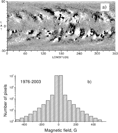
Figure 1: NSO/Kitt Peak solar magnetic flux data. (a) Sample synoptic map for Carrington rotation No. 1689; white represents positive polarity of magnetic field, and black represents negative polarity. (b) Distribution of magnetic flux values for 1976 – 2003. (For better viewing the limited range of $\pm 500$ G is presented.)

Synoptic maps have the following spatial resolution: $1^{\circ}$ in longitude (360 steps); 180 equal steps in the sine of the latitude from –1 (South pole) to +1 (North pole). Thus every map consists of $360\times 180$ pixels of magnetic flux values.

An example of a magnetic field synoptic map is presented in Figure 1a (Carrington rotation No. 1689). White represents the positive polarities of magnetic field and black the negative polarities. One can see that strong magnetic fields of both polarities occupy a relatively small part of the Sun’s surface. Most of the surface is covered by magnetic field of low magnetic flux density (various shades of gray).

This feature can be seen in Figure 1b, which depicts the magnetic field strength distribution for the whole period under consideration (1976 – 2003). A nearly symmetric distribution contains 98.7% of the values in the interval 0 – 100 G, whereas pixels with $B$ above 100 G occupy only 1.3% of the solar surface. (For better viewing the limited interval $|B|<500$ G is represented.) Even so, the total number of the latter pixels is large enough, amounting to $3\times 10^{5}$ for 1976 – 2003, and thus allowing detailed analysis of their distribution.

3 Method

To study the longitudinal distribution of the photospheric magnetic field we have used the following approach. For each $1^{\circ}$ interval of heliolongitude from $1^{\circ}$ to $360^{\circ}$, magnetic flux values were averaged over the selected latitude interval. Latitude-averaged values of $|B|$ were used to study the longitudinal magnetic field distribution. An example of the resulting longitudinal distribution for Carrington rotation No. 1689 is presented in Figure 2. The whole latitude interval (from –90^∘ to +90^∘) was used in this example. Two cases were considered separately: weak fields (pixels with $|B|<100$ G, Figure 2a) and strong fields ($|B|>100$ G, Figure 2b).

The longitudinal asymmetry of the photospheric magnetic field distribution was evaluated by means of the vector summation technique (Vernov et al., 1979; Vernova et al., 2002). Latitude-averaged values of $|\mathbf{b}_{i}|$ for each $1^{\circ}$ interval (from $1^{\circ}$ to $360^{\circ}$) were considered as vector modulus, with corresponding Carrington longitude being the phase angle of $\mathbf{b}_{i}$. Then resulting vector sum was calculated for every Carrington rotation as

$$\mathbf{B}=\sum\limits_{i=1}^{360}\mathbf{b}_{i}.$$

Whereas the modulus of $\mathbf{B}$ (of the resulting vector sum) can be considered as a measure of longitudinal asymmetry, the direction of the vector (phase angle) points to the Carrington longitude dominating during the given Carrington rotation. Long-term change of the longitudinal asymmetry as well as that of the total photospheric magnetic flux follow the 11-year solar cycle.

Vectors presented as arrows in Figure 2 show both values of the longitudinal asymmetry (vector modulus in relative units) and Carrington longitudes dominating in this rotation (vector phase angle). Two cases – weak fields (pixels with $|B|<100$ G, Figure 2a) and strong fields ($|B|>100$ G, Figure 2b) – were treated separately. The longitudinal distribution for the strong field contains distinct separate peaks, whereas the weaker field displays smoother longitude dependence. However, in spite of the visible difference in the general pattern, the resulting vectors of the longitudinal asymmetry have fairly close orientations in this example.

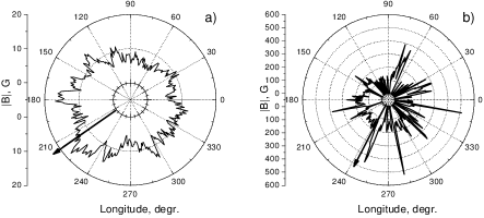
Figure 2: Polar diagrams of latitude-averaged magnetic field for (a) weak fields – pixels with $|B|<100$ G and (b) strong fields – pixels with $|B|>100$ G. Arrows represent longitudinal asymmetry of the distribution evaluated by means of the vector summation technique. In the figure vector length is given in relative units; direction points to the Carrington longitude dominating during the given rotation. A latitude interval from –90^∘ to +90^∘ was used in this example.

By means of this technique the dominating Carrington longitude was evaluated for each solar rotation. The longitudinal distribution of the photospheric magnetic field during 1976 – 2003 was studied on the basis of the time series obtained in this way. Only strong magnetic fields ($|B|>100$ G) were included further in our calculations. The latitude interval from –45^∘ to +45^∘ is considered throughout the rest of this paper. In addition to the combined distribution for both hemispheres data for the northern hemisphere (latitudes from $0^{\circ}$ to $+45^{\circ}$) and for the southern one (latitudes from $0^{\circ}$ to $-45^{\circ}$) were considered separately.

4 Two Patterns of Magnetic Field Longitudinal Distribution

While studying the sunspot longitudinal distributions corresponding to the four phases of the solar cycle (minimum, ascending phase, maximum, and descending phase), we have found considerable similarity between ascending phase and maximum (Vernova et al., 2004). The descending phase and minimum distributions on the other hand displayed a pattern drastically different from the one typical for two other phases of the solar cycle. Accordingly, we grouped the whole data set into two parts, one (to be called AM) consisting of the ascending phases and the maxima of the solar cycles included in the data set and the other (DM) consisting of the descending phases and the minima.

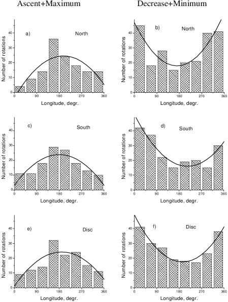
Figure 3: Two opposite patterns of magnetic field longitudinal distribution corresponding to the ascent and the maximum of solar cycle (left panels) and to the decrease and the minimum (right panels): (a), (b) northern hemisphere; (c), (d) southern hemisphere; (e), (f) solar disk. Histograms represent distributions of dominating longitudes (one value per Carrington rotation). Solid lines indicate the best-fitting second-order polynomial, drawn to emphasize the difference between two forms of envelope. Note that histograms for solar disk [(e) and (f)] do not represent the sum of the northern and southern hemisphere histograms. They were obtained by independently treating of the data from –45^∘ to +45^∘ in heliolatitude.

The same approach is used now in the study of the photospheric magnetic field distribution. Longitudinal distributions calculated by means of the technique described in Section 3 are presented in Figures 3a and b (northern hemisphere, latitudes from $0^{\circ}$ to $+45^{\circ}$), Figures 3c and d (southern hemisphere, latitudes from $0^{\circ}$ to $-45^{\circ}$), and Figures 3e and f (solar disk, latitudes from $-45^{\circ}$ to $+45^{\circ}$). These figures represent distributions of dominating longitudes (one value per Carrington rotation) for the following time intervals. All AM phases for the 1976 – 2003 period are combined in Figures 3a, c, and e and all DM phases are combined in Figures 3b, d, and f. We have taken into account only those Carrington rotations for which the asymmetry of the distribution was pronounced (i.e., the modulus of the resulting vector $\mathbf{B}$ was sufficiently large). This has reduced the sample only by about 10%.

Two opposite types of photospheric field longitudinal distribution can be seen for two parts of the 11-year cycle: convex – for the ascending phase and maximum (Figures 3a, c, and e) and concave – for the decrease and minimum (Figures 3b, d, and f). Accordingly the distribution maxima change from $180^{\circ}$ for the AM phase to $0^{\circ}/360^{\circ}$ for the DM phase. The best-fitting second-order polynomials were added in each case to emphasize the convex (maximum close to $180^{\circ}$ of Carrington longitude) or concave (maximum close to $0^{\circ}/360^{\circ}$ longitude) nature of the distribution. One can see in Figure 3 that two patterns of the longitudinal distribution appear in the northern and the southern hemispheres simultaneously indicating a synchronous development of the asymmetry in both solar hemispheres. Yet the distribution for the northern hemisphere depicts a less regular behavior than that for the southern hemisphere.

As was stated in Section 3, only strong magnetic fields are considered in this study. The chosen limit ($|B|>100$ G) makes it possible to observe the indicated phenomenon (two maxima separated by $180^{\circ}$) more clearly. The same effect can be seen, though it is less pronounced, when we lower the limit to $|B|>10-20$ G. It should be noted, however, that for weak fields (with $|B|<20$ G) the effect disappears completely; the longitudinal distribution is uniform within the range of statistical error.

The distributions in Figure 3 were constructed as a combination of data for several solar cycles, (i.e., the observed peculiarities point to long-lived longitudinal asymmetry distinguishable through averaging of long data sets). Our previous results (Vernova et al., 2004) obtained for the longitudinal sunspot distribution show that these distribution peculiarities go beyond the period 1976 – 2003. For the present article we treated anew the data set produced by the Greenwich observatory (http://solarscience.msfc.nasa.gov/greenwch.shtml) using the same method of vector summing (see Section 3) for the period 1917 – 2003. Each sunspot was represented as a vector: The vector modulus was set equal to the sunspot area and the direction of the vector (phase angle) was pointed to the Carrington longitude of the sunspot. As a result of vector summing, the dominating longitude for each solar rotation was obtained. In Figure 4 the longitudinal distributions of sunspots for AM and DM periods are presented. Here, as in the case of magnetic fields, the same patterns of the distribution can be seen (convex for the AM periods and concave for the DM ones). Thus, we see that, when the data are averaged over 8 solar cycles, the form of the distribution is preserved with the shift of the maximum by $180^{\circ}$ when passing from the AM period to the DM one.

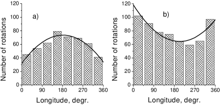
Figure 4: Sunspot longitudinal distribution (solar disk, 1917 – 2003): (a) the ascent and the maximum (AM) of solar cycle; (b) the decrease and the minimum (DM). Solid lines indicate the best-fitting second-order polynomials. Two opposite patterns can be seen for the AM and DM periods of the solar cycle.

That we have to deal with two parts of the same process can be illustrated in the following way. A distribution combining all magnetic field data for 1976 – 2003 was obtained by shifting the decrease–minimum data by $180^{\circ}$ and summing with the ascent–maximum distribution (Figure 5a). In the same way sunspot data for 1917 – 2003 were combined in a single distribution both for AM and DM periods (Figure 5b).

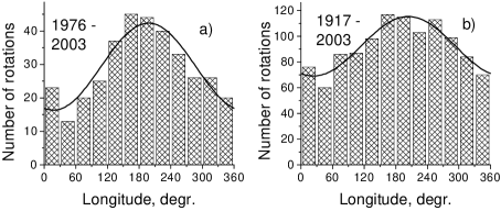
Figure 5: Combination of all data in a single distribution. The distribution for the ascent–maximum of solar cycle was combined with the decrease–minimum distribution shifted by $180^{\circ}$. (a) solar magnetic field, 1976 – 2003 (latitudes from –45^∘ to +45^∘), and (b) sunspots, 1917 – 2003. Solid lines are the best-fitting sine curves.

The resulting modified histograms depict a very systematic (almost sinusoidal) behavior of the longitudinal distribution with a pronounced maximum at about $180^{\circ}$. In spite of long data sets under consideration, the resulting histograms display extraordinary large and smooth variations. Best-fitting sinusoids were added to Figures 5a and b. The maximum of the fitting sinusoid is located at $198\pm 7^{\circ}$ longitude for the magnetic field (Figure 5a) and at $204\pm 7^{\circ}$ longitude for the sunspot distribution (Figure 5b). A chi-square test shows that the probability for the pattern appearing from random fluctuations of the uniform distribution is much less than 1% for both distributions (Figures 5a and b).

The present phenomenon manifests itself as a result of averaging over the period of 28 years for magnetic field and 87 years for sunspots. It shows the alternating domination of two large intervals of the longitudes: from $90^{\circ}$ to $270^{\circ}$ (with the maximum at $180^{\circ}$) for the AM period, and the opposite interval from $270^{\circ}$ to $90^{\circ}$ (the maximum at $0^{\circ}/360^{\circ}$) for the DM period. This effect does not exclude the clustering of solar activity in one, two, or more active zones, whose locations can be different from the maxima of the longitudinal asymmetry observed by us.

5 Magnetic Field Polarity and Active Longitudes

The times separating the two characteristic periods (AM and DM) are important intervals of the solar magnetic cycle. The time between the solar maximum and the beginning of the declining phase coincides with the inversion of the Sun’s global magnetic field whereas the time between the solar minimum and the ascending phase is related to the start of the new solar cycle and the change of the magnetic polarity of sunspots according to Hale’s law.

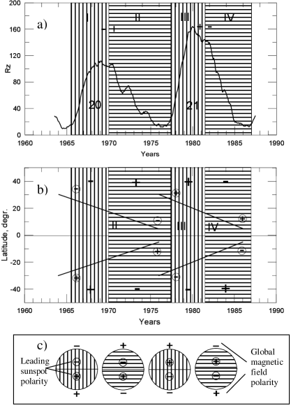
Figure 6: Change of global and local magnetic field polarities in the course of the solar magnetic cycle. (a) Example of two 11-year cycles (20th and 21st) forming a single magnetic cycle: solid line – Wolf number; I and III – ascent and maximum periods (vertical shading), II and IV – decrease and minimum (horizontal shading). Global magnetic field polarities are designated at the top of the panel for the North hemisphere. (b) Evolution of local magnetic fields during the same period. Solid lines show schematically the latitudinal drift of sunspots. Leading sunspot polarities are shown inside circles. Other notation is the same as in the panel (a). Global magnetic field polarities are designated at the top and at the bottom of the panel. (c) Scheme illustrating coincidence of global magnetic field polarity with the polarity of leading sunspots for periods I and III (ascent and maximum). Opposite polarities occur for periods II and IV (decrease and minimum).

The change of magnetic field polarities in the course of the 22-year solar cycle is illustrated by Figure 6, where two successive 11-year cycles are presented (by way of example, even cycle 20 and odd cycle 21 are considered). According to our approach each of the cycles is divided into two periods (ascent–maximum and decrease–minimum). Four corresponding periods I, II, III, and IV are separated by vertical lines (Figure 6a).

The polarity changes of both the global and the local solar magnetic fields are shown schematically in Figure 6b. The polarity of the leading sunspot is indicated inside the circles at the beginning and at the end of lines following the latitudinal displacement of the sunspot activity during the solar cycle. At the top and at the bottom of the panel the global magnetic field polarities are indicated for the northern and southern hemispheres, respectively.

Connection of the four periods I, II, III, and IV with the magnetic field polarities is depicted in Figure 6c. Big circles represent the Sun during the four periods, with global magnetic field polarity being indicated at the poles. Small circles represent schematically the leading sunspots and their polarity for the corresponding solar hemisphere.

Comparing the four diagrams in Figure 6c one can see that the two characteristic periods (AM and DM) correspond to different situations occurring in the 22-year magnetic cycle of the Sun, in the course of which the global magnetic field polarity and polarity of the leading sunspot may be the same (for each solar hemisphere) or opposite. During the ascending phase and the maximum (active longitude $180^{\circ}$) polarities of the global magnetic field and those of the leading sunspots coincide, whereas for the descending phase and the minimum (active longitude $0^{\circ}/360^{\circ}$) polarities are opposite.

Table 1: Solar magnetic field polarities and active longitudes

	North hemisphere		South hemisphere
Solar cycle	Global	Leading	Global	Leading	Active
phase	magnetic	sunspot	magnetic	sunspot	longitude
	field	polarity	field	polarity
Even cycle
Ascent–maximum	$-$	$-$	$+$	$+$	$180^{\circ}$
Decrease–minimum	$+$	$-$	$-$	$+$	$0^{\circ}$
Odd cycle
Ascent–maximum	$+$	$+$	$-$	$-$	$180^{\circ}$
Decrease–minimum	$-$	$+$	$+$	$-$	$0^{\circ}$

In Table 1 the polarity of the global magnetic field, polarity of the leading sunspot and longitudinal location of the magnetic field maximum are compared for periods I, II, III, and IV of the solar magnetic cycle. One can see that the maximum of the photospheric magnetic field distribution appeared at longitude $180^{\circ}$ during AM periods (I and III) in contrast to DM periods (II and IV) with the maxima at $0^{\circ}/360^{\circ}$.

Thus when the polarity of the global magnetic field and the polarity of the leading sunspot are the same (within one hemisphere) the longitudinal maximum is at $180^{\circ}$. However, when these polarities are opposite the maximum is at about $0^{\circ}/360^{\circ}$. One may suppose that the observed change of active longitudes is connected with the polarity changes of Sun’s magnetic field in the course of the 22-year magnetic cycle.

6 Longitudinal Distributions of Solar Activity

Analogous results were obtained by us earlier on the basis of Wilcox Solar Observatory (WSO) data for 1976 – 2004 (Vernova, Tyasto, and Baranov, 2005). For treating the WSO photospheric magnetic field data another technique was used instead of the vector summation used here for the Kitt Peak data. Latitude-averaged magnetic field values (latitudes from $-70^{\circ}$ to $+70^{\circ}$) for each solar rotation were analyzed and peaks exceeding a mean value by 1.5 standard deviations were selected. Longitudes corresponding to the positions of these peaks were used when plotting the magnetic field longitudinal distribution. In contrast to Kitt Peak data, no discrimination was made between strong and weak fields; that is, all measured values ($30\times 72$ pixels for each synoptic map) were included.

For both data sets two opposite types of longitudinal distributions corresponding to AM and DM periods were observed for the photospheric magnetic field, with maxima being situated at Carrington longitude $180^{\circ}$ during the AM period and at $0^{\circ}/360^{\circ}$ during the DM one.

Longitudinal distributions of many different manifestations of solar activity display the same features as those that are characteristic of the photospheric magnetic field distribution and sunspots. In the study of solar proton event sources (1976 – 2003) and X-ray flare sources (1976 – 2003) it was found that activity distributions behave differently during the ascending phase and the maximum of the solar cycle on the one hand and during the descending phase and the minimum on the other, depicting maxima around opposite Carrington longitudes ($180^{\circ}$ and $0^{\circ}/360^{\circ}$) (Vernova, Tyasto, and Baranov, 2005). Thus various manifestations of solar activity (sunspots, X-ray flares, and solar proton event sources), as well as the photospheric magnetic field show long-term asymmetry with similar features of heliolongitudinal distribution.

This phenomenon is seen more clearly when the vector summation method is used for data treatment as it was in cases of sunspots, Kitt Peak magnetic field data, and X-ray flare sources. Yet similar results were obtained in our studies with other kinds of treatment (sunspots, WSO magnetic field data, and solar proton event sources). It should be noted that, along with the phenomenon found by us, other types of longitudinal asymmetry may exist, and these could manifest themselves, for example, during shorter periods of time.

7 Discussion

The effects described here evidence the existence of a specific longitudinal asymmetry of the solar photospheric magnetic field distribution. On the one hand, this asymmetry is very stable; the maxima of the magnetic field distribution are observed at the same Carrington longitudes over a period of 1976 – 2003 (with the same feature persisting for 1917 – 2003 in the sunspot distribution). On the other hand, the maximum of distribution changes jump like its longitudinal position by $180^{\circ}$ twice during the 11-year solar cycle. The long-term stability of the distribution relative to Carrington coordinate frame can be interpreted as a manifestation of rigidly rotating magnetic field structure.

Of special interest is the regular change of the maximum position (around $180^{\circ}$ for the ascent and maximum period and $0^{\circ}/360^{\circ}$ for the decrease and minimum period) found by us earlier for the sunspot distribution (Vernova et al., 2004) and for other indices of solar activity (Vernova, Tyasto, and Baranov, 2005) and now confirmed by the analysis of the photospheric magnetic field data. The connection of the two characteristic periods with changes of the global magnetic field polarity and those of the leading sunspot polarities is unlikely to be a coincidence. It was shown by Benevolenskaya et al. (2002) that the relation of the polarity of the Sun’s global magnetic field to the sign of the following sunspots is of principal importance. Using soft X-ray data from the Yohkoh X-ray telescope for the period of 1991 – 2001 they discovered giant magnetic loops connecting the magnetic flux of the following parts of the active regions with the magnetic flux of the polar regions that have the opposite polarity. These large-scale magnetic connections appeared mostly during the rising phase of the solar cycle and its maximum. These connections did not appear or were very weak during the declining phase of the solar cycle. Thus the two characteristic periods AM and DM correspond to radically different patterns of the large-scale magnetic field of the Sun.

The features of the magnetic field distribution described here are in good accordance with those previously reported by us for the solar activity distribution. This coincidence points to the asymmetry of the solar magnetic field distribution being the cause of the corresponding longitudinal asymmetry of various manifestations of the solar activity. It should be noted that all cases displayed a broad maximum of the longitudinal distribution, which does not conform with the idea of active longitudes having an extent of about $20^{\circ}$ – $60^{\circ}$, see, e.g., Benevolenskaya et al. (1999). It is possible that some smoothing of the distribution can be attributed to averaging over the long time interval. Yet other authors have also pointed out a similar pattern of the longitudinal asymmetry. Balthasar and Schüssler (1983) observed the longitudinal asymmetry of sunspot groups as the predominance of one of the solar hemispheres as compared with the other one.

Both for solar activity manifestations (Vernova et al., 2004) and for the photospheric magnetic field (this study) the maxima of distributions were observed near the heliolongitudes $180^{\circ}$ and $0^{\circ}/360^{\circ}$. It was noted by many authors that active longitudes tend to appear on diametrically opposite sides of the Sun.

Analysis of the solar activity for 1962 – 1966 has shown that centers of activity have a tendency to develop on opposite sides of the Sun (Dodson and Hedeman, 1968). In studies of the longitudinal distribution of the major solar flares, active zones separated by $180^{\circ}$ were found, where the flare occurrence rate was much higher (Bai, 1987).

In some cases increased manifestations of activity were found near the longitudes $180^{\circ}$ and $0^{\circ}/360^{\circ}$ (Dodson and Hedeman, 1968; Bumba et al., 1996; Jetsu et al., 1997). In Jetsu et al. (1997) a search for periodicity was performed in major solar flare data during three decades (1956 – 1985). For combined data of both hemispheres two active longitudes rotating with a constant synodic period of 22.07 days were observed at about $0^{\circ}$ and $180^{\circ}$. One should especially mention the work of Skirgiello (2005), where increased activity of heliolongitudes $180^{\circ}$ and $30^{\circ}$ was discovered on the basis of the CME data; moreover, these nearly antipodal longitudes dominated alternately. Similar to our observations, the domination of the longitude $180^{\circ}$ coincided with the AM phase of the solar cycle, whereas the domination of the longitude $30^{\circ}$ coincided with the DM phase. In agreement with our study of the sunspot distribution (Vernova et al., 2004), the author points out for the CME distribution a more distinct manifestation of the active longitudes for the southern hemisphere of the Sun.

The transition from the AM period to the DM one, which coincides with the inversion of Sun’s global magnetic field, is accompanied by radical changes in longitudinal distribution of the solar activity. Simultaneously with the change of the activity maximum position by $180^{\circ}$, the relative value of the asymmetry of the northern and the southern hemispheres changes too. On the basis of the sunspot data we have shown that during the period of the inversion a transition from domination of the northern hemisphere to domination of the southern hemisphere occurs (Vernova et al., 2002). Similar features were found by Kane (2005) when studying the solar flare index: During cycles 21 and 22 the transition from a multiyear northern preference to a multiyear southern preference was observed around or after the polarity reversal.

8 Conclusion

Longitudinal distributions of the photospheric magnetic field studied on the basis of National Solar Observatory (Kitt Peak) data (1976 – 2003) displayed two opposite patterns during different parts of the 11-year solar cycle. Heliolongitudinal distributions differed for the ascending phase and the maximum of the solar cycle on the one hand, and for the descending phase and the minimum on the other, depicting maxima around two opposite Carrington longitudes ($180^{\circ}$ and $0^{\circ}/360^{\circ}$). Thus the maximum of the distribution shifted its position by $180^{\circ}$ with the transition from one characteristic period to the other.

The same peculiarities of the longitudinal distribution were observed for the photospheric magnetic field studied on the basis of Wilcox Solar Observatory data (1976 – 2004), sunspot data (1917 – 2003); solar proton event sources (1976 – 2003), and X-ray flare sources (1976–2003).

Two characteristic periods correspond to different situations occurring in the 22-year magnetic cycle of the Sun, in the course of which the global magnetic field polarity and polarity of the leading sunspot may be the same (in each solar hemisphere) or opposite. During the ascending phase and the maximum (active longitude $180^{\circ}$) polarities of the global magnetic field and those of the leading sunspots coincide, whereas for the descending phase and the minimum (active longitude $0^{\circ}/360^{\circ}$) the polarities are opposite. Thus radical change of longitudinal distribution may be connected with reorganization of solar magnetic field in the course of the 22-year magnetic cycle.

The ”classical” solar dynamo model is axisymmetric and therefore does not explain the longitudinal asymmetry of the solar activity distribution. The longitudinal asymmetry does not show itself in such a regular and evident form as the latitudinal development of the solar activity. That is why, up to a certain point, models of the solar cycle simply ignored this aspect of the solar activity distribution. Now the bulk of observational data confirming the existence of active longitudes is so large that this phenomenon should be accounted for in a complete model of the solar cycle. Efforts were made to explain the appearance of modes in the solar cycle that are non-symmetric with respect to the axis ( e.g., Gilman and Fox, 1997; Dikpati and Gilman, 2005). Peter Gilman in his talk ”A 42 Year Quest to Understand the Solar Dynamo and Predict Solar Cycles” (Gilman, 2006) expressed hope that ”a unified theory of the solar cycle and active longitudes” will be produced in the near future.