Revision of VLT/UVES constraints on a varying fine-structure constant

Abstract

We critically review the current null results on a varying fine-structure constant, $\alpha$, derived from VLT/UVES quasar absorption spectra, focusing primarily on the many-multiplet analysis of 23 absorbers from which Chand et al. (2004) reported a weighted mean relative variation of $\hbox{$\Delta\alpha/\alpha$}=(-0.06\pm 0.06)\times 10^{-5}$. Our analysis of the same reduced data, using the same fits to the absorption profiles, yields very different individual $\Delta\alpha/\alpha$ values with uncertainties typically larger by a factor of $\sim$3. We attribute the discrepancies to flawed parameter estimation techniques in the original analysis and demonstrate that the original $\Delta\alpha/\alpha$ values were strongly biased towards zero. Were those flaws not present, the input data and spectra should have given a weighted mean of $\hbox{$\Delta\alpha/\alpha$}=(-0.44\pm 0.16)\times 10^{-5}$. Although this new value does reflect the input spectra and fits (unchanged from the original work – only our analysis is different), we do not claim that it supports previous Keck/HIRES evidence for a varying $\alpha$: there remains significant scatter in the individual $\Delta\alpha/\alpha$ values which may stem from the overly simplistic profile fits in the original work. Allowing for such additional, unknown random errors by increasing the uncertainties on $\Delta\alpha/\alpha$ to match the scatter provides a more conservative weighted mean, $\hbox{$\Delta\alpha/\alpha$}=(-0.64\pm 0.36)\times 10^{-5}$. We highlight similar problems in other current UVES constraints on varying $\alpha$ and argue that comparison with previous Keck/HIRES results is premature.

1 Introduction

Absorption lines from heavy element species in distant gas clouds along the sight-lines to background quasars (QSOs) are important probes of possible variations in the fine-structure constant, $\alpha$, over cosmological time- and distance-scales. The many-multiplet (MM) method (Dzuba et al., 1999; Webb et al., 1999) utilizes the relative wavelength shifts expected from different transitions in different neutral and/or ionized metallic species to measure $\alpha$ with an order of magnitude better precision than previous techniques such as the alkali doublet (AD) method. It yielded the first tentative evidence for $\alpha$-variation (Webb et al., 1999) and subsequent, larger samples saw this evidence grow in significance and internal robustness (Murphy et al. 2001a; Webb et al. 2001; Murphy, Webb & Flambaum 2003, hereafter M03). MM analysis of 143 absorption spectra, all from the Keck/HIRES instrument, currently indicate a smaller $\alpha$ in the clouds at the fractional level $\hbox{$\Delta\alpha/\alpha$}=(-0.57\pm 0.11)\times 10^{-5}$ over the redshift range $0.2<\hbox{$z_{\rm abs}$}<4.2$ (Murphy et al., 2004, hereafter M04). Clearly, this potentially fundamental result must be refuted or confirmed with many different spectrographs to guard against subtle systematic errors which, despite extensive searches (Murphy et al. 2001b; M03), have evaded detection so far.

First attempts at constraining $\alpha$-variation with the Ultraviolet and Visual Echelle Spectrograph (UVES) on the Very Large Telescope (VLT) in Chile have, at first glance, yielded null results. The MM constraints in the literature are summarized by Fig. 1, the caption of which describes several important caveats for interpreting the figure.

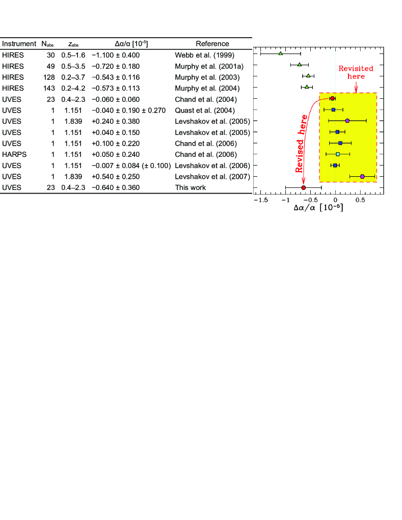
Figure 1: Summary of the many-multiplet constraints on $\Delta\alpha/\alpha$ in the literature. The table shows the instrument used, the sample size (N_abs), the absorption redshift (or range), the value of $\Delta\alpha/\alpha$ with 1-$\sigma$ error (for statistical samples, the weighted mean value and its 1-$\sigma$ error are quoted) and the corresponding references. The plot allows easy comparison of the $\Delta\alpha/\alpha$ values and their 1-$\sigma$ errors but there are several important caveats the reader should note: (i) We demonstrate in this paper that some UVES and HARPS constraints are based on flawed parameter estimation techniques and are not reliable. The reliability of other UVES constraints is also questioned in this work; (ii) Many points are not independent. Points in the plot with the same symbols use the same data (to varying extents); (iii) The sample sizes are very different. Some samples contain only a single absorption system; random errors for statistical samples are systematic errors for single absorbers; (iv) The redshift ranges vary considerably. If $\alpha$ does vary from absorber to absorber then that information is lost here; (v) The typical signal-to-noise ratio of the spectra in each sample is different; (vi) Some error-bars on $\Delta\alpha/\alpha$ contain a systematic component which is combined with the statistical one into a single error term. Other points contain no systematic error term. Quast et al. (2004) quote a separate systematic term. Levshakov et al. (2006) do calculate a systematic term but do not quote it together with the statistical term.

To date, the only MM analysis of a statistically significant UVES sample is that of Chand et al. (2004, hereafter C04; summarize the main results) who reported that $\hbox{$\Delta\alpha/\alpha$}=(-0.06\pm 0.06)\times 10^{-5}$ from 23 absorbers in the redshift range $0.4<\hbox{$z_{\rm abs}$}<2.3$. The main aim of the current paper is to revise these results after demonstrating simple flaws in the data analysis technique of C04. The same flaws are also evident in the AD analysis of Chand et al. (2005) who reported a weighted mean $\hbox{$\Delta\alpha/\alpha$}=(+0.15\pm 0.43)\times 10^{-5}$ from 15 Si iv doublets over the range $1.5<\hbox{$z_{\rm abs}$}<3.0$.

Different MM analyses of 2 individual absorption clouds for which higher signal-to-noise ratio (${\rm S/N}$) spectra are available have also provided seemingly strong constraints on $\Delta\alpha/\alpha$. Null results with 1-$\sigma$ statistical uncertainties of $0.19$, $0.15$ and $0.24\times 10^{-5}$ were derived by Quast et al. (2004), Levshakov et al. (2005) and Chand et al. (2006), respectively, from UVES spectra of the complex $\hbox{$z_{\rm abs}$}=1.151$ absorber towards HE 0515$-$4414. The constraint of Chand et al. (2006) again suffers from the same data analysis errors as the statistical results in C04. Levshakov et al. (2006, hereafter L06) improved their earlier constraints (from Quast et al. 2004 and Levshakov et al. 2005) to $\hbox{$\Delta\alpha/\alpha$}=(-0.007\pm 0.084)\times 10^{-5}$. We demonstrate here that the UVES data utilized in that analysis simply do not allow such a low statistical uncertainty. The other individual high-${\rm S/N}$ absorber analysed with the MM method is at $\hbox{$z_{\rm abs}$}=1.839$ towards Q 1101$-$264. Recently, Levshakov et al. (2007, hereafter L07) revised their earlier constraint (Levshakov et al., 2005) from $\hbox{$\Delta\alpha/\alpha$}=(0.20\pm 0.38)\times 10^{-5}$ to $\hbox{$\Delta\alpha/\alpha$}=(0.54\pm 0.25)\times 10^{-5}$ by analysing new spectra with higher resolution. We discuss this result further in Section 4.

As mentioned above, the main focus of this paper is to critically analyse the reliability of the C04 results, the only statistical MM study apart from our previous Keck/HIRES work. In Section 2 we point out problems in the ‘$\chi^{2}$-curve’ measurement technique used by C04. We also introduce a simple algorithm for estimating the minimum statistical error in $\Delta\alpha/\alpha$ achievable from any given absorption spectrum. The uncertainties quoted by C04 are inconsistent with this ‘limiting precision’. In Section 3 we revise the C04 results using the same spectral data but with robust numerical algorithms which we demonstrate are immune to the errors evident in C04. Section 4 discusses the other constraints on $\Delta\alpha/\alpha$ from UVES mentioned above. We conclude in Section 5.

2 Motivations for revising UVES results

2.1 $\chi^{2}$ curves

$\Delta\alpha/\alpha$ is typically measured in a quasar absorption system using a $\chi^{2}$ minimization analysis of multiple-component Voigt profiles simultaneously fit to the absorption profiles of several different transitions. The column densities, Doppler widths and redshifts defining the individual components are varied iteratively until the decrease in $\chi^{2}$ between iterations falls below a specified tolerance, $\Delta\chi^{2}_{\rm tol}$. Our approach in Murphy et al. (2001a), M03 & M04 was simply to add $\Delta\alpha/\alpha$ as an additional fitting parameter, to be varied simultaneously with all the other parameters in order to minimize $\chi^{2}$. The approach of C04, following Webb et al. (1999), was to keep $\Delta\alpha/\alpha$ as an external parameter: for a fixed input value of $\Delta\alpha/\alpha$ the other parameters of the fit are varied to minimize $\chi^{2}$. The input value of $\Delta\alpha/\alpha$ is stepped along over a given range around zero and $\chi^{2}$ is computed at each step. The functional form of $\chi^{2}$ implies that, in the vicinity of the best-fitting $\Delta\alpha/\alpha$, the ‘$\chi^{2}$ curve’ – the value of $\chi^{2}$ as a function of the input value of $\Delta\alpha/\alpha$ – should be near parabolic and smooth. In practice, this means that in each separate fit, with a different input $\Delta\alpha/\alpha$, $\Delta\chi^{2}_{\rm tol}$ should be set to $\ll 1$ to ensure that any fluctuations on the final $\chi^{2}$ curve are also $\ll 1$. This is obviously crucial when using the standard method of deriving the 1-$\sigma$ uncertainty, $\delta(\hbox{$\Delta\alpha/\alpha$})$, from the width of the $\chi^{2}$ curve at $\chi^{2}_{\rm min}+1$: if the fluctuations on the $\chi^{2}$ curve are $\ga$$1$ then one expects $\chi^{2}_{\rm min}$ to be rather poorly defined and $\delta(\hbox{$\Delta\alpha/\alpha$})$ to be underestimated. The larger the fluctuations on the $\chi^{2}$ curve, the more the measured value of $\Delta\alpha/\alpha$ will deviate from the true value and, even worse, the more significantly it will deviate since its uncertainty will be more underestimated.

Even a cursory glance at the $\chi^{2}$ curves of C04 – figure 2 in Srianand et al. (2004), figure 14 in C04 itself – reveal that none could be considered smooth at the $\ll 1$ level and, almost without exception, the $\chi^{2}$ fluctuations significantly exceed unity (two examples are shown in Section 3.3 – see Fig. 5). Again, we stress that no matter how noisy the spectral data or how poorly one’s model profile fits the data or how many free parameters are being fitted, the $\chi^{2}$ curve should be smooth and near parabolic in the vicinity of the best fit. The $\chi^{2}$ fluctuations in C04 must therefore be due to failings in the algorithm used to minimize $\chi^{2}$ for each input $\Delta\alpha/\alpha$. This point can not be over-emphasized since the $\chi^{2}$ curve is the very means by which C04 measure $\Delta\alpha/\alpha$ and its uncertainty in each absorption system.

Based on fits to simulated absorption spectra, C04 argue that their measurement technique is indeed robust. However, strong fluctuations even appear in the $\chi^{2}$ curves for these simulations (their figure 2). This leads to spurious $\Delta\alpha/\alpha$ values: figure 6 in C04 shows the results from 30 realizations of a simulated single-component Mg/Fe ii absorber. At least 15 $\Delta\alpha/\alpha$ values deviate by $\geq 1\sigma$ from the input value; 8 of these deviate by $\geq 2\sigma$ and 4 by $\geq 3\sigma$. There is even a $\approx 5$-$\sigma$ value. The distribution of $\Delta\alpha/\alpha$ values should be Gaussian in this case but these outliers demonstrate that it obviously is not. The $\chi^{2}$ fluctuations also cause the uncertainty estimates, $\delta(\hbox{$\Delta\alpha/\alpha$})$, from each simulation to range over a factor of $\approx 4$ even though all realizations had the same simulated ${\rm S/N}$ and input parameters. None of these problems arise in our own simulations of either single- or multiple-component systems (Murphy 2002; M03).

Clearly, the results of C04 cannot be reliable if the $\chi^{2}$ minimization algorithm – the means by which $\Delta\alpha/\alpha$ and $\delta(\hbox{$\Delta\alpha/\alpha$})$ are measured – failed. From the discussion above, we should expect that their uncertainty estimates are underestimated as a result. The following sub-section demonstrates this by introducing a simple measure of the minimum possible $\delta(\hbox{$\Delta\alpha/\alpha$})$ in a given absorption system. We correct the analysis of C04 in Section 3 using the same data and profile fits.

2.2 A simple measure of the limiting precision on $\Delta\alpha/\alpha$

2.2.1 Formalism

  

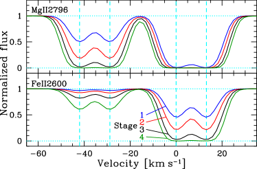
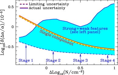
Figure 2: Left-hand panel: Simulation of two transitions in a multi-component absorber. Both transitions have the same velocity structure: two main spectral features, each comprising two blended velocity components with equal column densities. Labelled are distinct stages of differential saturation in the two main spectral features. Right-hand panel: The difference between the limiting precision, $\delta(\hbox{$\Delta\alpha/\alpha$})_{\rm lim}$, and the actual precision (as derived by $\chi^{2}$-minimization analysis) varies strongly from stage to stage. In a single-component absorber the actual uncertainty tracks $\delta(\hbox{$\Delta\alpha/\alpha$})_{\rm lim}$, as expected. See text for discussion.

The velocity shift, $\Delta v_{i}$, of transition $i$ due to a small variation in $\alpha$, i.e. $\hbox{$\Delta\alpha/\alpha$}\ll 1$, is determined by the $q$-coefficient for that transition,

$$\omega_{i}(z)\equiv\omega_{i}(0)+q_{i}\left[\left(\alpha_{z}/\alpha_{0}\right)^{2}-1\right]\,\hskip 10.00002pt\Rightarrow\hskip 10.00002pt\frac{\Delta v_{i}}{c}\approx-2\frac{\Delta\alpha}{\alpha}\frac{q_{i}}{\omega_{i}(0)}\,,$$ (1)

where $\omega_{i}(0)$ and $\omega_{i}(z)$ are the rest-frequencies in the laboratory and in an absorber at redshift $z$ respectively. Similarly, $\alpha_{0}$ and $\alpha_{z}$ are the laboratory and absorber values of $\alpha$. The MM method is the comparison of measured velocity shifts from several transitions (with different $q$-coefficients) to compute the best-fitting $\Delta\alpha/\alpha$. The linear equation (1) implies that the error in $\Delta\alpha/\alpha$ is determined only by the distribution of $q$-coefficients (assumed to have negligible errors) being used and the statistical errors in the velocity shifts, $\delta_{{\rm v},i}$:

$$\delta(\hbox{$\Delta\alpha/\alpha$})_{\rm lim}=\sqrt{S/D}\,,$$ (2)

where

$$S\equiv\sum_{i}\left(\frac{\delta_{{\rm v},i}}{c}\right)^{-2}$$ (3)

and

$$D\equiv S\sum_{i}\left(\frac{2q_{i}}{\omega_{i}(0)}\right)^{2}\left(\frac{\delta_{{\rm v},i}}{c}\right)^{-2}-\left[\sum_{i}\frac{2q_{i}}{\omega_{i}(0)}\left(\frac{\delta_{{\rm v},i}}{c}\right)^{-2}\right]^{2}\,.$$ (4)

This expression is just the solution to a straight-line least-squares fit, $y=a+bx$, to data $(x_{j},y_{j})$, with errors only on the $y_{j}$, where the intercept $a$ is also allowed to vary. Allowing the intercept to vary is important since it mimics the real situation in fitting absorption lines where the absorption redshift and $\Delta\alpha/\alpha$ must be determined simultaneously.

Equation (2) can only be used if one knows the statistical error on the velocity shift measurement for each transition, $\delta_{{\rm v},i}$. This quantity is only well-defined in an absorption system with a single fitted velocity component or in a system with several velocity components which do not blend or overlap significantly with each other. However, the general case – and, observationally, by far the most common one – is that absorbers have many velocity components which, at the resolution of the spectrograph, are strongly blended together. For this general case we wish to define a ‘total velocity uncertainty’ for each transition integrated over the absorption profile (i.e. over all components), $\sigma_{{\rm v},i}$, so that the substitution $\delta_{{\rm v},i}=\sigma_{{\rm v},i}$ in equation (2) provides some easily-interpreted information about $\delta(\hbox{$\Delta\alpha/\alpha$})_{\rm lim}$.

The quantity $\sigma_{{\rm v},i}$ is commonly used in radial-velocity searches for extra-solar planets, e.g. Bouchy et al. (2001), but is not normally useful in QSO absorption-line studies. Most metal-line QSO absorption profiles display a complicated velocity structure and one usually focuses on the properties of individual velocity components, each of which is typically modelled by a Voigt profile. However, it is important to realize that $\Delta\alpha/\alpha$ and its uncertainty are integrated quantities determined by the entire absorption profile. Some velocity components – typically the narrow, deep-but-unsaturated, isolated ones – will obviously provide stronger constraints than others but all components nevertheless contribute something. Thus, $\sigma_{{\rm v},i}$ should incorporate all the velocity-centroiding information available from a given profile shape. From a spectrum $F(k)$ with 1-$\sigma$ error array $\sigma_{F}(k)$, the minimum possible velocity uncertainty contributed by pixel $k$ is given by (Bouchy et al., 2001)

$$\frac{\sigma_{\rm v}(k)}{c}=\frac{\sigma_{F}(k)}{\lambda(k)\,\left[\partial F(k)/\partial\lambda(k)\right]}\,.$$ (5)

That is, a more precise velocity measurement is available from those pixels where the flux has a large gradient and/or a small uncertainty. This quantity can be used as an optimal weight, $W(k)\equiv\left[\sigma_{\rm v}(k)/c\right]^{-2}$, to derive the total velocity precision available from all pixels in a portion of spectrum,

$$\textstyle\sigma_{\rm v}=c\left[\sum_{k}W(k)\right]^{-1/2}\,.$$ (6)

For each transition in an absorber, $\sigma_{{\rm v},i}$ is calculated from equations (5) & (6). Note that the only requirements are the 1-$\sigma$ error spectrum and the multi-component Voigt profile fit to the transition’s absorption profile. The latter allows the derivative in (5) to be calculated without the influence of noise. If very high ${\rm S/N}$ spectra are available – i.e. where the $\sigma_{F}(k)$ are always much less than the flux difference between neighbouring pixels in high-gradient portions of the absorption profiles – then one could use the spectrum itself instead of the Voigt profile fit, thus making the estimate of $\sigma_{\rm v}$ model-independent. Once $\sigma_{{\rm v},i}$ has been calculated for all transitions $i$, the uncertainty in $\Delta\alpha/\alpha$ simply follows from equation (2) with the substitution $\delta_{{\rm v},i}=\sigma_{{\rm v},i}$.

2.2.2 Limiting precision

It is important to realize that the uncertainty calculated with the above method represents the absolute minimum possible 1-$\sigma$ error on $\Delta\alpha/\alpha$; the real error – as derived from a simultaneous $\chi^{2}$-minimization of all parameters comprising the Voigt profile fits to all transitions – will always be larger than $\delta(\hbox{$\Delta\alpha/\alpha$})_{\rm lim}$ from equation (2). The main reason for this is that absorption systems usually have several velocity components which have different optical depths in different transitions. Equation (2) assumes that the velocity information integrated over all components in one transition can be combined with the same integrated quantity from another transition to yield an uncertainty on $\Delta\alpha/\alpha$. However, in a real determination of $\Delta\alpha/\alpha$, each velocity component (or group of components which define a sharp spectral feature) in one transition is, effectively, compared with only the same component (or group) in another transition.

Figure 2 illustrates this important point. It shows simulated absorption profiles for two transitions commonly used in MM analyses (Mg ii $\lambda$2796 and Fe ii $\lambda$2600) in different stages of saturation. The velocity structure is identical for both transitions and contains two well-separated main spectral features (MSFs), each of which comprises two velocity components which are blended together. The column-density ratios between the corresponding components of the two transitions is kept fixed while the total column density is varied. For each simulation with a different total column density we determined $\delta(\hbox{$\Delta\alpha/\alpha$})_{\rm lim}$ using the method above and the real value of $\delta(\hbox{$\Delta\alpha/\alpha$})$ using the usual $\chi^{2}$ minimization analysis. When comparing $\delta(\hbox{$\Delta\alpha/\alpha$})_{\rm lim}$ with $\delta(\hbox{$\Delta\alpha/\alpha$})$ one notices 4 characteristic stages as the column density increases:

• Stage 1: Both MSFs are relatively unsaturated in both transitions and so $\sigma_{{\rm v},i}$ will be small for $i$=Mg ii $\lambda$2796 and $i$=Fe ii $\lambda$2600. Thus, $\delta(\hbox{$\Delta\alpha/\alpha$})_{\rm lim}$ is quite small. However, note that the right-hand MSF in Mg ii $\lambda$2796 is nevertheless a little saturated and so the real precision is somewhat weakened, i.e. $\delta(\hbox{$\Delta\alpha/\alpha$})$ is pushed higher than $\delta(\hbox{$\Delta\alpha/\alpha$})_{\rm lim}$; the high velocity precision available from that MSF in Fe ii $\lambda$2600 is ‘wasted’ because the profile of the corresponding MSF in Mg ii $\lambda$2796 is smoother.

• Stage 2: The right-hand MSF in Mg ii $\lambda$2796 is now completely saturated. Since that part of the profile is now smoother, $\delta(\hbox{$\Delta\alpha/\alpha$})_{\rm lim}$ should get larger. However, this is more than compensated by the additional centroiding potential (or velocity information) now offered by the weaker velocity components in the left-hand MSF and both MSFs in Fe ii $\lambda$2600 due to the increased column density. On the other hand, the real precision, $\delta(\hbox{$\Delta\alpha/\alpha$})$, has substantially worsened because the right-hand MSF from the two transitions no longer constrain $\Delta\alpha/\alpha$ tightly when considered together. This principle also applies to the left-hand MSF where, in Fe ii $\lambda$2600, it is too weak to provide strong constraints, even though the same velocity components in Mg ii $\lambda$2796 are stronger and well-defined.

• Stage 3: The decrease in $\delta(\hbox{$\Delta\alpha/\alpha$})_{\rm lim}$ is now dominated by the small increase in velocity information available from the left-hand MSF because the right-hand MSF of both transitions is now saturated. Note also that the real precision also improves here because the components of the left-hand MSF in Fe ii $\lambda$2600 are getting stronger while the corresponding components of Mg ii $\lambda$2796 are not completely saturated.

• Stage 4: The decrease in $\delta(\hbox{$\Delta\alpha/\alpha$})_{\rm lim}$ is now only marginal because it is dominated only by one MSF in one transition, i.e. the left-hand side of Fe ii $\lambda$2600. However, $\delta(\hbox{$\Delta\alpha/\alpha$})$ has increased sharply because now even the left-hand MSF of Mg ii $\lambda$2796 is saturated and, when considered together with the corresponding MSF of Fe ii $\lambda$2600, provides no constraint on $\Delta\alpha/\alpha$.

To summarize this illustration, it is always the case that $\delta(\hbox{$\Delta\alpha/\alpha$})_{\rm lim}<\delta(\hbox{$\Delta\alpha/\alpha$})$ and it is the degree of differential saturation between corresponding components of different transitions which determines how much worse $\delta(\hbox{$\Delta\alpha/\alpha$})$ is than $\delta(\hbox{$\Delta\alpha/\alpha$})_{\rm lim}$. Also note that the ${\rm S/N}$ of the data (or the simulations above) affects $\delta(\hbox{$\Delta\alpha/\alpha$})_{\rm lim}$ and $\delta(\hbox{$\Delta\alpha/\alpha$})$ in precisely the same way. That is, the ratio $\delta(\hbox{$\Delta\alpha/\alpha$})_{\rm lim}/\delta(\hbox{$\Delta\alpha/\alpha$})$ is independent of ${\rm S/N}$. Only the degree of differential saturation between corresponding components of different transitions affects $\delta(\hbox{$\Delta\alpha/\alpha$})_{\rm lim}/\delta(\hbox{$\Delta\alpha/\alpha$})$.

Finally, as the above discussion implies, fits comprising a single velocity component (or multiple but well separated components) should have $\delta(\hbox{$\Delta\alpha/\alpha$})_{\rm lim}\approx\delta(\hbox{$\Delta\alpha/\alpha$})$. As an internal consistency check on our simulations, Fig. 2 also shows the results for an absorber with a single velocity component, again in the Mg ii $\lambda$2796 and Fe ii $\lambda$2600 transitions. Note that $\delta(\hbox{$\Delta\alpha/\alpha$})_{\rm lim}$ tracks quite closely the real value of $\delta(\hbox{$\Delta\alpha/\alpha$})$ as a function of column density. Nevertheless, the real error is slightly worse than $\delta(\hbox{$\Delta\alpha/\alpha$})_{\rm lim}$; this is expected because the real estimate derives from a fit where all parameters of the absorption profiles, including the Doppler parameters and column densities, are varied simultaneously, thus slightly weakening the constraint on $\Delta\alpha/\alpha$ (and the absorber redshift).

2.2.3 Application to existing constraints on $\Delta\alpha/\alpha$

We have calculated $\delta(\hbox{$\Delta\alpha/\alpha$})_{\rm lim}$ for the absorbers from the three independent data-sets which constitute the strongest current constraints on $\Delta\alpha/\alpha$: (i) the 143 absorbers in our Keck/HIRES sample (M04); (ii) the 23 absorption systems, comprising mostly Mg/Fe ii transitions, from UVES studied by C04; (iii) the UVES exposures of the $z_{\rm abs}=1.151$ absorber towards HE 0515$-$4414 studied by L06. Calculating $\delta(\hbox{$\Delta\alpha/\alpha$})_{\rm lim}$ requires only the error spectra and the Voigt profile models used to fit the data. For samples (ii) & (iii) we use the Voigt profile models published by those authors. Below we describe the errors arrays. For sample (ii), other aspects of the data are important for the analysis in Section 3 and so we also describe them here.

The reduced (i.e. one-dimensional) spectra in sample (ii) were kindly provided to us by B. Aracil who confirmed that the wavelength and flux arrays are identical to those used in C04. However, one main difference is that the error arrays we use are generally a factor $\approx$1.4 smaller than those used by C04 (H. Chand, B. Aracil, 2006, private communication). We have confirmed this by digitizing the absorption profiles plotted in C04. The reason for this is that they derive their error arrays by adding two error terms of similar magnitude in quadrature, even though each term should reasonably approximate the actual error. One term reflects the formal photon statistics while the other reflects the r.m.s. variation in the flux from the different exposures which are combined to form the final spectrum. Our error spectra were derived from the maximum of the two terms. Thus, the error spectra of C04 are $\approx$1.3–2 times larger than ours. We have confirmed that our error arrays match well the r.m.s. flux in unabsorbed spectral regions; they therefore more accurately reflect the real uncertainty in flux for each spectral pixel. Note that this implies that $\delta(\hbox{$\Delta\alpha/\alpha$})_{\rm lim}$ calculated using our spectra will be smaller than the value C04 would derive. The only other difference between our spectra and those of C04 is that we performed our own continuum normalization of the absorption profiles. However, we used a method similar to that employed by C04 and any small differences will have negligible effects on the analysis here and in Section 3.

For sample (iii), we reduced the raw UVES exposures using a modified version of the UVES pipeline. For the present analysis, small differences between our reduction and that of L06 are unimportant; all that is required is that the error arrays match fairly closely. Indeed, the ${\rm S/N}$ matches very well those quoted by L06 in the relevant portions of the reduced spectrum.

For all samples, the atomic data for the transitions (including $q$-coefficients) were the same as used by the original authors.

In practice, when applying equations (5) and (6) we sub-divide the absorption profile of each transition into $15{\rm\,km\,s}^{-1}$ chunks to mitigate the effects illustrated in Fig. 2. This provides a value of $\delta(\hbox{$\Delta\alpha/\alpha$})_{{\rm lim},j}$ for each chunk $j$. The final value of $\delta(\hbox{$\Delta\alpha/\alpha$})_{\rm lim}$ is simply $\{\sum_{j}1/[\delta(\hbox{$\Delta\alpha/\alpha$})_{{\rm lim},j}]^{2}\}^{1/2}$; in all cases this is $<$1.4 times the value obtained without sub-divisions.

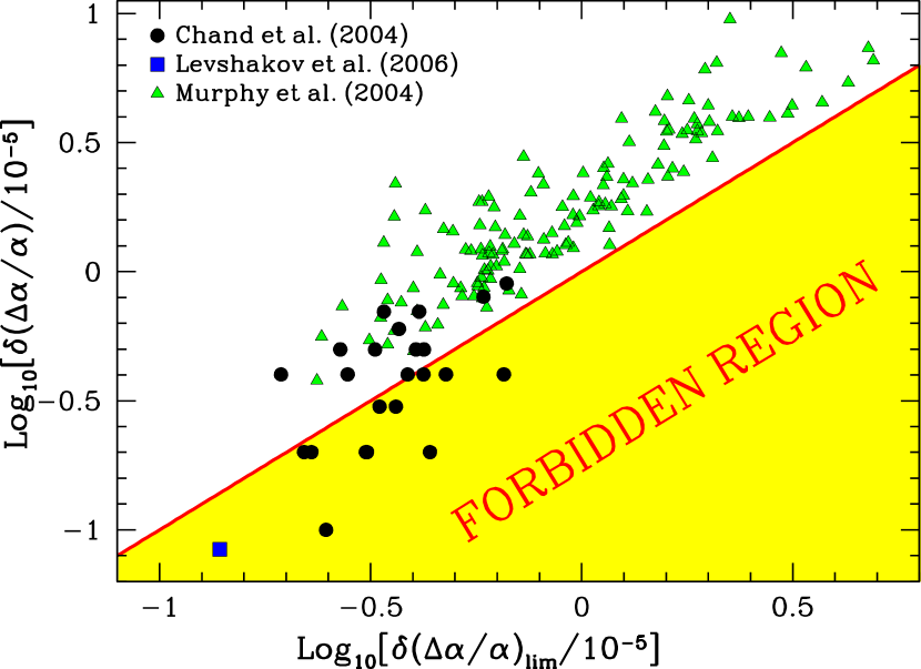
Figure 3: Quoted errors on $\Delta\alpha/\alpha$ versus the limiting precision, $\delta(\hbox{$\Delta\alpha/\alpha$})_{\rm lim}$, for current samples. The Chand et al. (2004) and Levshakov et al. (2006) samples fail the basic requirement that $\delta(\hbox{$\Delta\alpha/\alpha$})$ must be greater than $\delta(\hbox{$\Delta\alpha/\alpha$})_{\rm lim}$.

Figure 3 shows the 1-$\sigma$ error on $\Delta\alpha/\alpha$ quoted by the original authors versus the limiting precision, $\delta(\hbox{$\Delta\alpha/\alpha$})_{\rm lim}$. The main results are clear. Firstly, the 1-$\sigma$ errors quoted for the HIRES sample in M04 always exceed $\delta(\hbox{$\Delta\alpha/\alpha$})_{\rm lim}$, as expected if the former are robustly estimated. Secondly, for at least 11 of their 23 absorbers, C04 quote errors which are smaller than $\delta(\hbox{$\Delta\alpha/\alpha$})_{\rm lim}$. Recall that since their error arrays are larger than ours, 11 out of 23 is a conservative estimate; if they were to calculate $\delta(\hbox{$\Delta\alpha/\alpha$})_{\rm lim}$ using their larger error arrays then more points on Fig. 3 would shift to the right into the ‘forbidden region’ where $\delta(\hbox{$\Delta\alpha/\alpha$})<\delta(\hbox{$\Delta\alpha/\alpha$})_{\rm lim}$. Finally, the very small error quoted by L06 for HE 0515$-$4414, $0.084\times 10^{-5}$, disagrees significantly with the limiting precision of $0.14\times 10^{-5}$. Thus, the (supposedly) strong current UVES constraints on $\Delta\alpha/\alpha$ fail a basic consistency test which not only challenges the precision reported by C04 and L06 but which must bring into question the robustness and validity of their analysis and final $\Delta\alpha/\alpha$ values.

As discussed in Section 2.1, underestimated error bars on $\Delta\alpha/\alpha$ are expected from the jagged $\chi^{2}$ curves derived by C04. Now we explore what effect the fluctuations had on the values of $\Delta\alpha/\alpha$ themselves and their uncertainties by applying a robust $\chi^{2}$ minimization algorithm.

3 Correcting the analysis of Chand et al. (2004)

3.1 Analysis method

  

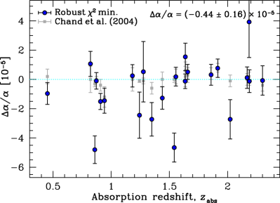
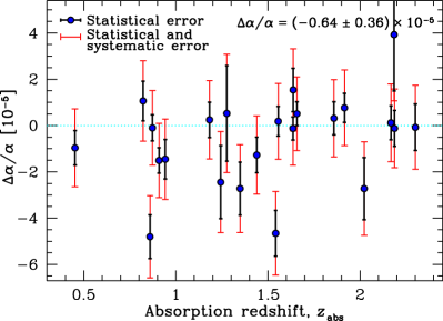
Figure 4: Left: Our new results (filled circles) are inconsistent with those of Chand et al. (2004) (grey squares) even though the same reduced data and profile fits were used. The only difference is that our $\chi^{2}$ minimization procedure is robust. The weighted mean $\hbox{$\Delta\alpha/\alpha$}=(-0.44\pm 0.16)\times 10^{-5}$ is consistent with our previous HIRES results but the scatter in the new results indicate remaining systematic errors in the data and fits. Right: To account for this additional scatter, we increase 1-$\sigma$ errors by adding a constant amount in quadrature such that the final $\chi^{2}_{\nu}=1$ about the weighted mean. The most conservative weighted mean result therefore becomes $\hbox{$\Delta\alpha/\alpha$}=(-0.64\pm 0.36)\times 10^{-5}$.

It is crucial to emphasize from the beginning here that we use the same spectra as C04 for the following analysis. To be precise, we use the same values of the flux with precisely the same wavelength scale, while Section 2.2.3 details why our error arrays are somewhat ($\sim$30 per cent) smaller than those of C04. Our aim is to establish the results that would have been obtained from the data had the $\chi^{2}$ minimization algorithm used by C04 not failed. For this reason we also fitted the same velocity structures to the data as C04. That is, for each absorption system, the best-fitting Voigt profile parameters of C04 were treated as first guesses in our $\chi^{2}$ minimization procedure. This is necessary because the Voigt profile parameters they report are not truly the best fitting ones (because their $\chi^{2}$ minimization algorithm failed). Nevertheless, the ‘qualitative’ aspects of the fits – i.e. the number and approximate relative positions of the constituent velocity components – remained the same throughout our subsequent $\chi^{2}$ minimization; it is in this sense that we state above that our “velocity structures” are the same as those of C04. Finally, the relationships between the Doppler widths of corresponding velocity components in different transitions were also the same as in C04.

The analysis procedure was the same as that described in detail in M03. The Voigt profile fitting and $\chi^{2}$ minimization are carried out within vpfit, a non-linear least-squares program designed specifically for analysing quasar absorption spectra, modified to include a single value of $\Delta\alpha/\alpha$ as a free parameter for each absorption system (Murphy, 2002). The relative tolerance for halting the $\chi^{2}$ minimization was set to $\Delta\chi^{2}_{\rm tol}/\chi^{2}=2\times 10^{-7}$ (i.e. small enough that, even for profile fits with thousands of degrees of freedom, $\Delta\chi^{2}$ is still $\ll 1$). Extensive simulations have confirmed the reliability of this approach (Murphy 2002; M03). The atomic data for the different transitions (i.e. laboratory wavelengths, oscillator strengths etc.) were identical to those used by C04.

Since $\Delta\alpha/\alpha$ is a free parameter, its value is determined directly during the $\chi^{2}$ minimization of each absorber and its uncertainty, $\delta(\hbox{$\Delta\alpha/\alpha$})$, is derived from the appropriate diagonal term of the final covariance matrix. As mentioned above, our error spectra are significantly smaller (though more appropriate) than those of C04 and so the final $\chi^{2}$ per degree of freedom in the fit, $\chi^{2}_{\nu}$, is typically $\approx$1.5–4 rather than $\approx$1 as would be expected if the model fit was appropriate (see Section 3.4 for further discussion). vpfit therefore increases $\delta(\hbox{$\Delta\alpha/\alpha$})$ by a factor of $\sqrt{\chi^{2}_{\nu}}$ and these are the values we report here. Simulations similar to those discussed in Murphy (2002) and M03 confirm that such a treatment yields very robust uncertainty estimates (see also Section 3.3).

3.2 Results

Table 1: Comparison of results from Chand et al. (2004) and this paper. Columns 1 & 2 give the J2000 and B1950 quasar names; the quasar emission redshifts are given in column 3. Column 4 gives the redshifts of the absorption systems. Columns 5 & 6 give the values from Chand et al. (2004) of $\Delta\alpha/\alpha$ and $\chi^{2}$ per degree of freedom, $\chi^{2}_{\nu}$, for the absorption profile fit. Columns 7 & 8 give the results of our attempt to reproduce those values. Column 9 gives our estimate of the wavelength calibration errors derived using the method of Murphy et al. (2007). All uncertainty estimates are 1-$\sigma$.

Quasar name		$z_{\rm em}$	$z_{\rm abs}$	Chand et al. (2004)		This work		$(\hbox{$\Delta\alpha/\alpha$})_{\rm ThAr}$
J2000	B1950			$\Delta\alpha/\alpha$ [$10^{-5}$]	$\chi^{2}_{\nu}$	$\Delta\alpha/\alpha$ [$10^{-5}$]	$\chi^{2}_{\nu}$	[$10^{-5}$]
J000344$-$232355	HE 0001$-$2340	$2.280$	$0.4524$	$\phantom{+}0.2\pm 0.5$	$1.10$	$-0.963\pm 0.747$	$3.27$	$-0.260\pm 0.093$
J000344$-$232355	HE 0001$-$2340	$2.280$	$2.1854$	$\phantom{+}0.2\pm 0.3$	$1.15$	$\phantom{+}3.926\pm 2.431$	$2.16$	$\phantom{+}0.145\pm 0.099$
J000344$-$232355	HE 0001$-$2340	$2.280$	$2.1872$	$-0.2\pm 0.2$	$1.20$	$-0.122\pm 0.774$	$2.10$	$-0.089\pm 0.099$
J000448$-$415728	Q 0002$-$422	$2.760$	$1.5419$	$\phantom{+}0.0\pm 0.2$	$0.66$	$-4.655\pm 0.988$	$1.00$	$-0.090\pm 0.103$
J000448$-$415728	Q 0002$-$422	$2.760$	$2.1679$	$\phantom{+}0.0\pm 0.4$	$1.03$	$\phantom{+}0.115\pm 0.731$	$0.78$	$-0.102\pm 0.069$
J000448$-$415728	Q 0002$-$422	$2.760$	$2.3006$	$-0.4\pm 0.4$	$0.99$	$-0.075\pm 1.001$	$2.54$	$-0.066\pm 0.086$
J011143$-$350300	Q 0109$-$3518	$2.410$	$1.1827$	$\phantom{+}0.0\pm 0.8$	$0.98$	$\phantom{+}0.249\pm 0.764$	$1.70$	$\phantom{+}0.011\pm 0.107$
J011143$-$350300	Q 0109$-$3518	$2.410$	$1.3489$	$-0.6\pm 0.4$	$1.08$	$-2.724\pm 1.144$	$2.28$	$\phantom{+}0.091\pm 0.083$
J012417$-$374423	Q 0122$-$380	$2.189$	$0.8221$	$\phantom{+}0.0\pm 0.9$	$0.87$	$\phantom{+}1.062\pm 0.859$	$2.27$	$-0.088\pm 0.078$
J012417$-$374423	Q 0122$-$380	$2.189$	$0.8593$	$-0.3\pm 0.2$	$1.29$	$-4.803\pm 0.941$	$2.81$	$\phantom{+}0.027\pm 0.078$
J012417$-$374423	Q 0122$-$380	$2.189$	$1.2433$	$-0.1\pm 0.1$	$0.89$	$-2.447\pm 1.579$	$4.10$	$\phantom{+}0.376\pm 0.095$
J024008$-$230915	PKS 0237$-$23	$2.223$	$1.6359$	$\phantom{+}0.2\pm 0.7$	$0.82$	$-0.124\pm 0.498$	$2.00$	$-0.062\pm 0.105$
J024008$-$230915	PKS 0237$-$23	$2.223$	$1.6372$	$\phantom{+}0.6\pm 0.6$	$1.16$	$\phantom{+}1.539\pm 0.939$	$2.93$	$\phantom{+}0.054\pm 0.068$
J024008$-$230915	PKS 0237$-$23	$2.223$	$1.6574$	$\phantom{+}0.3\pm 0.5$	$0.92$	$\phantom{+}0.510\pm 0.514$	$2.29$	$\phantom{+}0.121\pm 0.127$
J045523$-$421617	Q 0453$-$423	$2.660$	$0.9084$	$-0.4\pm 0.4$	$1.82$	$-1.507\pm 0.549$	$4.21$	$-0.141\pm 0.122$
J045523$-$421617	Q 0453$-$423	$2.660$	$1.8584$	$\phantom{+}0.4\pm 0.4$	$1.13$	$\phantom{+}0.315\pm 0.712$	$3.77$	$\phantom{+}0.467\pm 0.118$
J134427$-$103541	HE 1341$-$1020	$2.134$	$0.8728$	$\phantom{+}0.0\pm 0.2$	$1.19$	$-0.100\pm 0.567$	$2.49$	$-0.065\pm 0.071$
J134427$-$103541	HE 1341$-$1020	$2.134$	$1.2767$	$-0.1\pm 0.2$	$1.01$	$\phantom{+}0.524\pm 2.062$	$4.30$	$\phantom{+}0.531\pm 0.097$
J134427$-$103541	HE 1341$-$1020	$2.134$	$1.9154$	$\phantom{+}0.8\pm 0.3$	$1.49$	$\phantom{+}0.767\pm 0.627$	$2.08$	$\phantom{+}0.058\pm 0.072$
J135038$-$251216	HE 1347$-$2457	$2.534$	$1.4393$	$\phantom{+}0.0\pm 0.5$	$1.10$	$-1.272\pm 0.767$	$4.60$	$\phantom{+}0.024\pm 0.114$
J212912$-$153841	PKS 2126$-$158	$3.268$	$2.0225$	$-0.1\pm 0.4$	$1.19$	$-2.725\pm 1.344$	$2.65$	$\phantom{+}0.034\pm 0.111$
J222006$-$280323	HE 2217$-$2818	$2.406$	$0.9425$	$-1.2\pm 0.7$	$0.90$	$-1.453\pm 0.852$	$2.43$	$-0.258\pm 0.114$
J222006$-$280323	HE 2217$-$2818	$2.406$	$1.5558$	$\phantom{+}0.2\pm 0.5$	$1.22$	$\phantom{+}0.183\pm 0.639$	$2.93$	$-0.112\pm 0.114$

The best-fitting values of $\Delta\alpha/\alpha$ and the 1-$\sigma$ uncertainties, $\delta(\hbox{$\Delta\alpha/\alpha$})$, are compared with those of C04 in Fig. 4(left). Table 1 provides the numerical results. Many of the $\Delta\alpha/\alpha$ values are significantly different to those of C04, typically deviating from zero by much larger amounts. Moreover, our uncertainty estimates are almost always larger, usually by a significant margin (even though, again, our error spectra are consistently smaller than those employed by C04). The formal weighted mean over the 23 absorbers is

$$\hbox{$\Delta\alpha/\alpha$}=(-0.44\pm 0.16)\times 10^{-5}\,.$$ (7)

At first glance, this indicates a significantly smaller $\alpha$ in the absorption clouds compared to the laboratory value and agrees well with our previous results from HIRES. However, Fig. 4(left) also reveals significant scatter in the results well beyond what is expected based on our estimates of $\delta(\hbox{$\Delta\alpha/\alpha$})$: the value of $\chi^{2}$ about the weighted mean is $77.6$ which, for 22 degrees of freedom, has a probability of just $4\times 10^{-8}$ of being larger. It is therefore unclear whether these new results support our previous HIRES results or not. Further evidence is provided in Section 3.3 that these results do indeed reflect the reduced data and profile fits of C04 and that the discrepancy with their results is due to strong biases in both their $\Delta\alpha/\alpha$ and $\delta(\hbox{$\Delta\alpha/\alpha$})$ values. Systematic errors likely to affect the spectra are also discussed.

If we regard the large additional scatter in the new results as evidence of some additional random error then we can estimate its magnitude by adding a constant amount in quadrature to the current errors such that the final $\chi^{2}$ about the weighted mean becomes unity per degree of freedom. The additional random error required is $1.51\times 10^{-5}$. Figure 4(right) shows the new results with error bars which include the additional error term. Using these increased error bars, the weighted mean becomes

$$\hbox{$\Delta\alpha/\alpha$}=(-0.64\pm 0.36)\times 10^{-5}\,.$$ (8)

This value is the most conservative estimate of $\Delta\alpha/\alpha$ given the reduced data and profile fits of C04 as inputs. A similar procedure for dealing with increased scatter (beyond that expected from the purely statistical error bars) was followed in several previous works (Webb et al. 1999; M03; Tzanavaris et al. 2005, 2007). In Section 3.4 we discuss the possible origin of the large additional scatter, concluding that the profile fits of C04 are probably too simplistic. Indeed, this would lead to an additional systematic error for each absorption system which is random in sign and magnitude from absorber to absorber. That is, the assumptions underlying the derivation of equation (8) above are fairly realistic.

3.3 Biases in previous results

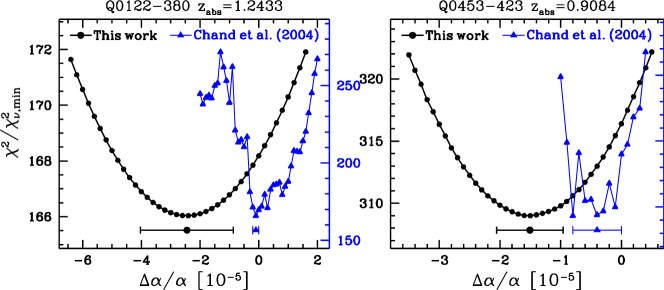
Figure 5: Example $\chi^{2}$ curves from our minimization algorithm (black circles, left-hand vertical scales) compared with those of Chand et al. (2004) (grey/blue triangles, right-hand vertical scales) which are simply reproduced from their figure 14. Fluctuations in the latter indicate failings in the minimization routine. Also note that sometimes (e.g. right-hand panel) the minima of C04’s curves are not well-defined due to these fluctuations. The points and error-bars at the minima indicate best-fitting values and 1-$\sigma$ uncertainties; for our curves they are from the algorithm where $\Delta\alpha/\alpha$ is a free parameter. The vertical scales are normalized by the minimum value of $\chi^{2}$ per degree of freedom (the C04 values of $\chi^{2}_{\nu}$ are reported in their table 3). Thus, the two curves on each panel have the same value at their minima since this is simply the number of degrees of freedom, $\nu$, by construction. However, C04’s curves rise much faster away from $\hbox{$\Delta\alpha/\alpha$}=0$ because the minimization algorithm fails to find the true minimum $\chi^{2}$ at each step in $\Delta\alpha/\alpha$. This may be the cause of the strong evident bias towards zero in C04’s values of $\Delta\alpha/\alpha$ (see Section 3.3).

Part of our motivation for revising the analysis of C04 was the large fluctuations in their $\chi^{2}$ curves. Although we include $\Delta\alpha/\alpha$ as a free parameter in our $\chi^{2}$ minimization process, treating it as an external parameter instead (as in C04) is a simple matter. As discussed in Section 2.1, a valid measurement of $\Delta\alpha/\alpha$ and (especially) $\delta(\hbox{$\Delta\alpha/\alpha$})$ can only come from a smooth, near parabolic, $\chi^{2}$ curve. The importance of this point is obvious in Fig. 5 which shows our $\chi^{2}$ curves in two example absorbers. For all 23 absorbers, we recover smooth, near parabolic $\chi^{2}$ curves, the minima of which coincide well with the values of $\Delta\alpha/\alpha$ plotted in Fig. 4. The two examples in Fig. 5 are no exceptions. Furthermore, the values of $\delta(\hbox{$\Delta\alpha/\alpha$})$ recovered from the width of the $\chi^{2}$ curves near their minima agree with the values recovered from the covariance matrix analysis discussed in Section 3.1. Thus, it is clear that our $\chi^{2}$ minimization procedure returns robust values of $\Delta\alpha/\alpha$ and $\delta(\hbox{$\Delta\alpha/\alpha$})$.

In contrast, Fig. 5 also shows the $\chi^{2}$ curves of C04, digitized from their figure 14, for the two example absorbers. The large $\chi^{2}$ fluctuations are obvious and it is clear that they cause two effects: (i) as already discussed, the 1-$\sigma$ uncertainties, $\delta(\hbox{$\Delta\alpha/\alpha$})$, are underestimated and (ii) the values of $\Delta\alpha/\alpha$ themselves may be biased towards zero.

The first effect is easy to understand: the minimum $\chi^{2}$ must, by definition, be found in a downward extreme fluctuation. Since the fluctuations are $\ga$1, the width of the ‘curve’ at $\chi^{2}_{\rm min}+1$ will be underestimated, typically by factors of order a few. The absorber at $z_{\rm abs}=1.2433$ towards Q0122$-$380, shown in Fig. 5(left), is the extreme example of this problem. The $\chi^{2}$ fluctuations are $\sim$10 here, leading C04 to assign an uncertainty of just $\delta(\hbox{$\Delta\alpha/\alpha$})=0.1\times 10^{-5}$ for this system. Note that different points on their $\chi^{2}$ curve are separated by this value so, even in principle, such an error estimate is questionable. Our robust error estimate is almost a factor of 16 times larger. Also note that it is far from clear how C04 determine $\delta(\hbox{$\Delta\alpha/\alpha$})$ in some absorbers. One such case is shown in Fig. 5(right) where, following the previous example, $\Delta\alpha/\alpha$ would appear to be $(-0.8\pm 0.1)\times 10^{-5}$ rather than the value quoted by C04, $(-0.4\pm 0.4)\times 10^{-5}$. In a few absorbers, such as this one, the confusion inherent in deriving $\delta(\hbox{$\Delta\alpha/\alpha$})$ from such jagged $\chi^{2}$ curves may have somewhat ameliorated potentially gross underestimates; in others, not.

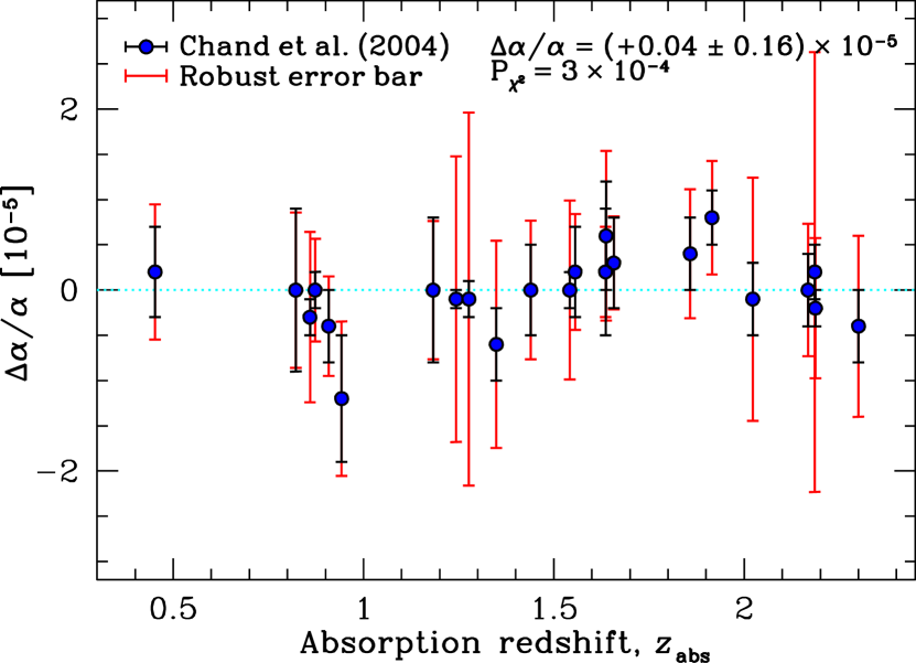
Figure 6: The 1-$\sigma$ uncertainties from our analysis (grey/red bars) compared with those of Chand et al. (2004) (black bars). The tight distribution of $\Delta\alpha/\alpha$ values from Chand et al. (2004) has a probability of just $P_{\chi^{2}}=3\times 10^{-4}$ of occurring by chance given our new robust error estimates.

The second effect – that the $\Delta\alpha/\alpha$ values of C04 are biased towards zero – is more difficult to understand. First, to demonstrate that the effect is significant, Fig. 6 shows the values of $\Delta\alpha/\alpha$ from C04 plotted with the 1-$\sigma$ uncertainties from our analysis. The $\Delta\alpha/\alpha$ values are clearly more tightly clustered around zero than expected based on our robust error-bars: the value of $\chi^{2}$ around the weighted mean of $\hbox{$\Delta\alpha/\alpha$}=(0.04\pm 0.16)\times 10^{-5}$ is just $6.1$. For 22 degrees of freedom, a $\chi^{2}$ this low (or lower) has a probability of only $P_{\chi^{2}}=3\times 10^{-4}$ of occurring by chance alone. The explanation for such a strong bias may be linked, again, to the failure of the $\chi^{2}$ minimization algorithm of C04. One possibility is that, for a given absorber, the minimization algorithm may have been run several times with $\Delta\alpha/\alpha$ fixed to zero with very slightly different initial conditions (as one might do when experimenting with different velocity structures in the model fit), thus reducing $\chi^{2}$ to a relatively low value even though the algorithm was impaired. When subsequently using non-zero values of $\Delta\alpha/\alpha$ in individual minimizations, the perturbation which the small shift in $\alpha$ imparts to the fit could cause $\chi^{2}$ to preferentially fluctuate to higher values. The impaired minimization algorithm may or may not repair this fluctuation (i.e. reduce $\chi^{2}$ by adjusting the parameters of the fit); this ‘hysteresis’ would therefore bias $\Delta\alpha/\alpha$ towards zero.

3.4 Likely systematic errors

Although Fig. 5 demonstrates the robustness of our $\Delta\alpha/\alpha$ and $\delta(\hbox{$\Delta\alpha/\alpha$})$ estimates, the large scatter of the results in Fig. 4 is inconsistent with our previous HIRES results. Furthermore, the HIRES values had a scatter consistent with that expected from the $\delta(\hbox{$\Delta\alpha/\alpha$})$ estimates (e.g. Webb et al. 1999; ; ). What systematic effects might contribute to the additional scatter in Fig. 4?

We considered a wide variety of systematic effects on $\Delta\alpha/\alpha$ in Murphy et al. (2001b) and M03, the most obvious possibility being wavelength calibration errors. The quasar spectra are wavelength calibrated by comparison with exposures of a thorium-argon (ThAr) emission-line lamp. A simple test for miscalibration effects was described in Webb et al. (1999) and applied to the HIRES data in Murphy et al. (2001b) and M03: the basic approach was to treat the ThAr emission lines near the redshifted quasar absorption lines to the same MM analysis, thereby deriving a correction, $(\hbox{$\Delta\alpha/\alpha$})_{\rm ThAr}$, to the value of $\Delta\alpha/\alpha$ in each absorber. For the HIRES spectra, wavelength calibration errors contributed negligible corrections, especially since so many absorption systems (128) were used (M03).

This ThAr test was not applied to the results of C04. However, recently in Murphy et al. (2007) we found that corruptions of the input list of ThAr wavelengths caused significant distortions of the wavelength scale in UVES spectra such as those of C04. From these distortions it is possible to quantify the value of $(\hbox{$\Delta\alpha/\alpha$})_{\rm ThAr}$ and it was demonstrated in Murphy et al. (2007) that the absorber at $z_{\rm abs}=1.2433$ towards Q0122$-$380 [Fig. 5(left)] was, again, particularly problematic, having $(\hbox{$\Delta\alpha/\alpha$})_{\rm ThAr}=+0.4\times 10^{-5}$. This is 4 times larger than the formal uncertainty quoted by C04 for this system. However, for most absorbers the corrections due to wavelength calibration errors are small compared to the scatter in Fig. 4; other systematic errors must dominate.

Another strong possibility is that too few velocity components have been fitted to the absorption profiles in many of the 23 absorbers. If this is the case then one should expect to find values of $\chi^{2}_{\nu}$ for the profile fits exceeding $\approx$1, whereas C04 generally found $\chi^{2}_{\nu}\sim 1$ for their fits. However, as mentioned several times above, the error spectra employed by C04 were set too high by a factor of $\approx$1.3–2. This is easily cross-checked by comparing the r.m.s. flux in continuum regions around the absorption profiles with the 1-$\sigma$ error spectra. Thus, when more appropriate error arrays are employed, as in our new analysis, the velocity structures of C04 prove too simplistic, resulting in the high values of $\chi^{2}_{\nu}\approx 1.5$–4 we derive. Clearly – and, in many cases, this is obvious simply upon visual inspection – more velocity components must be fitted in almost all 23 absorption systems to account for the evident velocity structure that the high $\chi^{2}_{\nu}$ values reflect. Preliminary fits which include additional velocity components indicate that ‘under-fitting’ of the absorption profiles has indeed caused large, spurious excursions in $\Delta\alpha/\alpha$ and may well be responsible for the bulk of the scatter in Fig. 4. The following Section presents a discussion and simulations of complicated velocity structures which confirm this.

4 Other constraints from UVES spectra

  

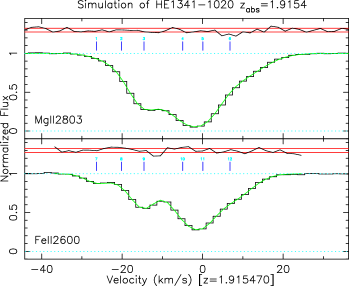
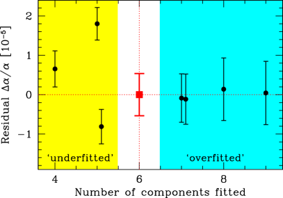
Figure 7: Fitting a simulated absorption profile with different numbers of velocity components. Left: Two transitions from the simulation showing the 6-component profile (green/grey curve) used to generate the synthetic data with $\hbox{${\rm S/N}$}=200$ per 2.5-${\rm km\,s}^{-1}$ pixel (black histogram). When under-fitting the data, we removed either or both the second and fourth components from the left. When over-fitting we added weak components around $-10$ and $10$–$20$ ${\rm km\,s}^{-1}$. Right: Values of $\Delta\alpha/\alpha$ obtained from the $\chi^{2}$ minimization. For each velocity structure (i.e. each fit with a different number and/or placement of components) we plot the mean value of $\Delta\alpha/\alpha$ and its standard deviation over 1000 realizations of the simulated data (the mean 1-$\sigma$ uncertainty from the realizations was also very close to the standard deviation). Note the large scatter in $\Delta\alpha/\alpha$ when the profile is fitted with fewer components than really present (‘under-fitted’) and the small scatter when it is ‘over-fitted’.

As mentioned in Section 1, several other recent studies of UVES QSO spectra have ostensibly provided constraints on $\Delta\alpha/\alpha$. The first of these was the AD analysis of 15 Si iv doublets by Chand et al. (2005). However, the $\chi^{2}$ curves they present contain strong fluctuations just like those in C04 – see their figures 1–6. It is therefore with caution that their final weighted mean result of $\hbox{$\Delta\alpha/\alpha$}=(+0.15\pm 0.43)\times 10^{-5}$ ($1.5<\hbox{$z_{\rm abs}$}<3.0$) should be interpreted. Our analysis of a sample of 21 somewhat lower ${\rm S/N}$ Si iv absorbers from Keck/HIRES gave $\hbox{$\Delta\alpha/\alpha$}=(-0.5\pm 1.3)\times 10^{-5}$ over the range $2.0<\hbox{$z_{\rm abs}$}<3.1$ without similar problems in minimizing $\chi^{2}$ for each absorber (Murphy et al., 2001c).

In Section 2.2.3 we saw that the MM analysis of the single complex $\hbox{$z_{\rm abs}$}=1.151$ absorber towards HE 0515$-$4414 by L06 gave a very small uncertainty of $\delta(\hbox{$\Delta\alpha/\alpha$})=0.084\times 10^{-5}$ but that the limiting precision was substantially larger, $\delta(\hbox{$\Delta\alpha/\alpha$})_{\rm lim}=0.14\times 10^{-5}$. However, in this case, we cannot easily identify the cause of the inconsistency. Nevertheless, it is quite possible, even likely, that the cause of the underestimated uncertainty also affected the value of $\Delta\alpha/\alpha$ and, again, caution should evidently be used in interpreting the result of L06. Previous analyses of the same absorber by the same group utilized very simplistic profile fits: see figure 2 of Quast et al. (2004), particularly at velocities around $-20$, $15$, $40$, $50$–$55$, $65$, $85\,\hbox{${\rm km\,s}^{-1}$}$ where large residuals are clearly visible. As we demonstrate below, these are very likely to have caused large systematic effects in this single-absorber estimate of $\Delta\alpha/\alpha$.

The same single absorber was studied, again with MM analysis, by Chand et al. (2006). However, in this case the fluctuations on the $\chi^{2}$ curve were so large – $\sim$50; see their figure 9 – that the authors found it difficult to define a minimum in the curve. Instead they attempted to fit a low-order polynomial through the large fluctuations – as one would fit a line through noisy data – to define a minimum. It must be strongly emphasized that such a practice is illogical and yields completely meaningless values of $\Delta\alpha/\alpha$ and $\delta(\hbox{$\Delta\alpha/\alpha$})$. Firstly, it is not ‘noise’ in the usual sense that one is attempting to fit through but spurious fluctuations in $\chi^{2}$ caused by the failure of the algorithm to find the true minimum at each fixed input value of $\Delta\alpha/\alpha$. Secondly, the real $\chi^{2}$ curve must lie beneath the majority of points on the $\chi^{2}$ and it cannot lie above any of them. The logical conclusion is that one cannot infer the shape, minimum or width – i.e. $\Delta\alpha/\alpha$ or $\delta(\hbox{$\Delta\alpha/\alpha$})$ – from such a $\chi^{2}$ curve since the real $\chi^{2}$ curve may lie anywhere below it.

The most recent constraint on $\Delta\alpha/\alpha$ from UVES QSO spectra was derived from MM analysis of the $\hbox{$z_{\rm abs}$}=1.839$ absorber towards Q 1101$-$264 by L07: $\hbox{$\Delta\alpha/\alpha$}=(+0.54\pm 0.25)\times 10^{-5}$. Three Fe ii transitions were employed – $\lambda$1608, $\lambda$2382 and $\lambda$2600. The latter two have nearly identical $q$-coefficients so they shift in concert as $\alpha$ varies. However, the bluer line, $\lambda$1608, shifts in the opposite sense to the other two and is therefore crucial for any meaningful constraint on $\Delta\alpha/\alpha$ to be derived. It is also the weaker line of the trio, with an oscillator strength less than a third of the others. As outlined in Section 3.4, systematic effects, even with small statistical samples of absorbers, can result if one does not fit the observed structure in the absorption profiles with an adequate number of velocity components. For any analysis of a single absorber, this becomes particularly important.

L07 explored this effect by using three different fits: a fiducial one with 16 velocity components and two others with fewer (11 and 10) components. They find very similar values of $\Delta\alpha/\alpha$ from all fits and therefore maintain that $\Delta\alpha/\alpha$ is insensitive to the number of fitted components. However, the components removed from the fiducial fit to form the 11- and 10-component fits appear mainly at the edges of the absorption complex and, crucially, do not absorb statistically significant fractions of the continuum in the weaker Fe ii $\lambda$1608 transition. That is, those components do not appear in Fe ii $\lambda$1608. Since this transition is vital to provide any sensitivity to $\alpha$ at all, one must find similar values of $\Delta\alpha/\alpha$ in all three fits; as far as $\Delta\alpha/\alpha$ is concerned, the three fits are identical and the test, in this case, is ineffective. In any case, visual inspection of the residuals between the fiducial fit and the data (figure 1 in L07, ) reveals correlations over $\sim$20-pixel ranges and, moreover, these ranges occur at similar velocities in the three different transitions. This is one indication of more than 16 components being required in the fit, not fewer. We will present further analysis of this absorber in Bainbridge et al. (in preparation).

To illustrate the effect of ‘under-fitting’ absorbers in this way, Fig. 7 shows a simulated absorption spectrum generated with 6 velocity components but which has then been fitted with different numbers of components. The Mg ii doublet ($\lambda\lambda$2796/2803) and the five strongest Fe ii transitions longward of 2340 Å were included in the fit but Fig. 7 just shows two representative transitions. All transitions were simulated with a ${\rm S/N}$ of 200 per 2.5-${\rm km\,s}^{-1}$ pixel in the continuum. The velocity structure was inspired by (but is not strictly the same as) a real absorption system – one of the 23 contained in the C04 sample – and includes two weaker components (the second and fourth from the left). It is these components which are missing in our 4- and 5-component fits to the simulated data. These fits result in values of $\Delta\alpha/\alpha$ which deviate significantly from the input value depending on which component is removed. Thus, ‘under-fitting’ individual absorption systems can easily cause spurious values of $\Delta\alpha/\alpha$.

With such high ${\rm S/N}$ ‘data’ we can also ‘over-fit’ the simulated absorption system. The additional components were placed at around $-10$ and $10$–$20$ ${\rm km\,s}^{-1}$. Of course, $\chi^{2}_{\nu}$ for these fits is below unity and, more importantly, the additional components are not statistically justified: the reduction in $\chi^{2}$ they provide compared to the fiducial 6-component fit is smaller than the additional number of free parameters they introduce. Nevertheless, the results show that the value of $\Delta\alpha/\alpha$ is robust to the introduction of these components. We hasten to add that one cannot simply keep fitting additional components: note that the uncertainty on $\Delta\alpha/\alpha$ increases as one adds components – with more components, $\chi^{2}$ becomes increasingly insensitive to $\Delta\alpha/\alpha$. However, when reporting strong constraints on $\Delta\alpha/\alpha$ from individual absorbers, some demonstration of how robust $\Delta\alpha/\alpha$ is to both under- and over-fitting is desirable and our illustration in Fig. 7 suggests that the latter is more conservative than the former.

5 Conclusion

We have critically analysed the reliability of the MM treatment of 23 VLT/UVES absorption systems by Chand et al. (2004, C04). Using the same data and profile fits we find values of $\Delta\alpha/\alpha$ in individual absorbers which deviate significantly from those of C04 and our uncertainty estimates are consistently and, in some cases dramatically, larger. Indeed, simple (but robust) calculations of the limiting precision available on $\Delta\alpha/\alpha$ in these absorbers indicates that $\ga$ half of C04’s quoted uncertainties are impossibly low; the ${\rm S/N}$ of the spectra and the complexity of the fitted velocity structures simply do not allow such small uncertainties on $\Delta\alpha/\alpha$.

This is altogether unsurprising given the large fluctuations in the $\chi^{2}$ curves presented by C04. The only way such large fluctuations can occur is if the $\chi^{2}$ minimization algorithm fails to reach a truly minimum value at each step along the input $\Delta\alpha/\alpha$ axis. That is, since the very means by which $\Delta\alpha/\alpha$ is estimated (the $\chi^{2}$ curve) is flawed, so are the values of $\Delta\alpha/\alpha$ and their uncertainties invalid. Just as the 1-$\sigma$ errors were underestimated, we have also demonstrated that C04’s values of $\Delta\alpha/\alpha$ are strongly biased towards zero. Again, this is likely to stem from the fluctuations on the $\chi^{2}$ curves.

It is therefore expected that C04’s weighted mean result of $\hbox{$\Delta\alpha/\alpha$}=(-0.06\pm 0.06)\times 10^{-5}$ should not truly represent the reduced data and profile fits they employed. Indeed, our own analysis – again, with the same reduced data and profile fits – yields a very different central value and much a larger error bar: $\hbox{$\Delta\alpha/\alpha$}=(-0.44\pm 0.16)\times 10^{-5}$. Since our $\chi^{2}$ minimization is demonstrably robust, we argue that this latter value does truly reflect the reduced data and profile fits. However, we do not argue that this value is necessarily the final or best one to be gleaned from this dataset: improvements in the profile fits are almost certainly required to reduce the evident scatter in the 23 values of $\Delta\alpha/\alpha$ to within that expected based on their (robust) 1-$\sigma$ uncertainties. Although not discussed in this paper, improvements in the data reduction process may also be needed. After increasing the uncertainties by adding a constant amount in quadrature to match the scatter, we obtain a more conservative estimate of the weighted mean from C04’s reduced data and profile fits: $\hbox{$\Delta\alpha/\alpha$}=(-0.64\pm 0.36)\times 10^{-5}$. Note that the uncertainty here is 6 times larger than that quoted by C04. The data and fits of C04 thus provide no stringent test of the Keck/HIRES evidence for a varying $\alpha$.

Jagged $\chi^{2}$ curves have also affected the AD analysis of Si iv doublets in UVES spectra by Chand et al. (2005) and the MM analysis of a single, high-${\rm S/N}$ UVES spectrum by Chand et al. (2006). The same single absorber was studied by Levshakov et al. (2006) but their quoted uncertainty is much lower than the limiting precision available, even in principle, from this spectrum. The only other UVES constraint on $\Delta\alpha/\alpha$ is from another single absorption system studied by Levshakov et al. (2007, L07). However, we have demonstrated that when analysing individual systems in this way, care must be taken to ensure that all the structure in the absorption profiles is adequately fitted. Indeed, simulations indicate ‘under-fitting’ the profile can cause dramatic spurious excursions from the real value of $\Delta\alpha/\alpha$ whereas ‘over-fitting’ the profile (to a mild degree) is a more conservative approach. We argue that additional components are probably required to fit the data of L07; this will be demonstrated in Bainbridge et al. (in preparation).

In summary, reliable comparison of HIRES and UVES constraints on a varying $\alpha$ must await improvements in the analysis of UVES spectra. We are currently reducing $>$100 UVES spectra to arrive at an internally and statistically robust estimate of $\Delta\alpha/\alpha$ for this purpose.

This paper has been typeset from a TeX/LaTeX file prepared by the author.

References

- Bouchy et al. (2001) Bouchy F., Pepe F., Queloz D., 2001, A&A, 374, 733
- Chand et al. (2005) Chand H., Petitjean P., Srianand R., Aracil B., 2005, A&A, 430, 47
- Chand et al. (2004) Chand H., Srianand R., Petitjean P., Aracil B., 2004, A&A, 417, 853 (C04)
- Chand et al. (2006) Chand H., Srianand R., Petitjean P., Aracil B., Quast R., Reimers D., 2006, A&A, 451, 45
- Dzuba et al. (1999) Dzuba V.A., Flambaum V.V., Webb J.K., 1999, Phys. Rev. Lett., 82, 888
- Levshakov et al. (2005) Levshakov S.A., Centurión M., Molaro P., D’Odorico S., 2005, A&A, 434, 827
- Levshakov et al. (2006) Levshakov S.A., Centurión M., Molaro P., D’Odorico S., Reimers D., Quast R., Pollmann M., 2006, A&A, 449, 879 (L06)
- Levshakov et al. (2007) Levshakov S.A., Molaro P., Lopez S., D’Odorico S., Centurión M., Bonifacio P., Agafonova I.I., Reimers D., 2007, A&A, 466, 1077 (L07)
- Murphy (2002) Murphy M.T., 2002, PhD thesis, Univ. New South Wales
- Murphy et al. (2004) Murphy M.T., Flambaum V.V., Webb J.K., Dzuba V. V., Prochaska J.X., Wolfe A.M., 2004, Lecture Notes Phys., 648, 131 (M04)
- Murphy et al. (2007) Murphy M.T., Tzanavaris P., Webb J.K., Lovis C., 2007, MNRAS, 378, 221
- Murphy et al. (2003) Murphy M.T., Webb J.K., Flambaum V.V., 2003, MNRAS, 345, 609 (M03)
- Murphy et al. (2001b) Murphy M.T., Webb J.K., Flambaum V.V., Churchill C. W., Prochaska J.X., 2001b, MNRAS, 327, 1223
- Murphy et al. (2001a) Murphy M.T., Webb J.K., Flambaum V.V., Dzuba V. A., Churchill C.W., Prochaska J.X., Barrow J.D., Wolfe A. M., 2001a, MNRAS, 327, 1208
- Murphy et al. (2001c) Murphy M.T., Webb J.K., Flambaum V.V., Prochaska J. X., Wolfe A.M., 2001c, MNRAS, 327, 1237
- Quast et al. (2004) Quast R., Reimers D., Levshakov S.A., 2004, A&A, 415, L7
- Srianand et al. (2004) Srianand R., Chand H., Petitjean P., Aracil B., 2004, Phys. Rev. Lett., 92, 121302
- Tzanavaris et al. (2007) Tzanavaris P., Murphy M.T., Webb J.K., Flambaum V.V., Curran S.J., 2007, MNRAS, 374, 634
- Tzanavaris et al. (2005) Tzanavaris P., Webb J.K., Murphy M.T., Flambaum V.V., Curran S.J., 2005, Phys. Rev. Lett., 95, 041301
- Webb et al. (1999) Webb J.K., Flambaum V.V., Churchill C.W., Drinkwater M. J., Barrow J.D., 1999, Phys. Rev. Lett., 82, 884
- Webb et al. (2001) Webb J.K., Murphy M.T., Flambaum V.V., Dzuba V. A., Barrow J.D., Churchill C.W., Prochaska J.X., Wolfe A. M., 2001, Phys. Rev. Lett., 87, 091301