Probing $\sim 100{\rm AU}$ Intergalactic Mg II Absorbing “Cloudlets” with Quasar Microlensing

Abstract

Intergalactic Mg II absorbers are known to have structures down to scales $\sim 10^{2.5}{\rm pc}$, and there are now indications that they may be fragmented on scales $\lesssim 10^{-2.5}{\rm pc}$ (Hao et al., astro-ph/0612409). When a lensed quasar is microlensed, the micro-images of the quasar experience creation, destruction, distortion, and drastic astrometric changes during caustic-crossing. I show that quasar microlensing can effectively probe Mg II and other absorption “cloudlets” with sizes $\sim 10^{-4.0}-10^{-2.0}{\rm pc}$ by inducing significant spectral variability on the timescales of months to years. With numerical simulations, I demonstrate the feasibility of applying this method to Q2237+0305, and I show that high-resolution spectra of this quasar in the near future would provide a clear test of the existence of such metal-line absorption “cloudlets” along the quasar sight line.

1 Introduction

Mg II absorbers towards the quasar sight lines have been systematically studied since Lanzetta et al. (1987) (for more recent studies, see Zibetti et al. 2005 and references therein). Similar Mg II absorbers were subsequently seen in gamma-ray burst (GRB) spectra. Prochter et al. (2006) compared GRB and quasar sight lines, and found a significantly higher incidence toward the former. They proposed three possible effects to explain this discrepancy: (1) faint quasars are obscured by dust associated with the absorbers; (2) Mg II absorbers are intrinsic to GRBs; (3) gravitational lensing of the GRB by the absorbers. However, they concluded that none of these effects provide a satisfactory explanation.

Frank et al. (2006) proposed a simple geometric solution to the puzzle. They argued that if Mg II absorption systems are fragmented on scales $\lesssim 10^{16}{\rm cm}$, similar to the beam sizes of GRBs, then the observed difference in incidence of Mg II absorbers would simply reflect the difference in the average beam sizes between GRBs and quasars, with quasars being on average several times as big. This explanation predicts that absorption features due to intervening Mg II cloud fragments should evolve as the size of GRB afterglow changes, which has now been observed by Hao et al. (2006). However, structures of the Mg II absorbers down to the size of $\sim 10^{16}{\rm cm}$ cannot be directly inferred from their spectral features. Rauch et al. (2002) put the strongest upper limits on Mg II absorber sizes to date. They observed the spectra of three images of Q2237+0305 (Huchra et al., 1985) and found that each line of sight contained individual Mg II absorbers at approximately the same redshift, but with distinct spectral features. Thus these absorbers are part of a complex that extends at least $\sim 500{\rm pc}$, but the sizes of the individual “cloudlets” must be smaller than $200-300{\rm pc}$ based on the separation of the macro-images.

Some, if not all, strongly lensed quasars are also gravitationally microlensed by the compact stellar-mass objects in the lensing galaxy (Wambsganss, 2006), and Q2237+0305 was the first lensed quasar to be found to exhibit significant microlensing variability (Corrigan et al., 1991; Woźniak et al., 2000). The macro-image of a microlensed quasar is split into many micro-images, and when the source moves over the caustic networks induced by the microlenses, those micro-images will expand, shrink, appear, disappear and experience drastic astrometric shifts over timescales of months or years (Treyer & Wambsganss, 2004). The angular sizes of major micro-images are usually of the same order as those of the quasars, and during the shape and position changes of these images, absorption structures of similar scale along their sight lines will likely imprint significant variations on the spectrum.

Brewer & Lewis (2005) pioneered the theoretical investigation of quasar microlensing as a probe of the sub-parsec structure of intergalactic absorption systems. They concluded that variation in the strength of the absorption lines over timescales of years or decades caused by microlensing can be used to probe the structures of Lyman $\alpha$ clouds and associated metal-line absorption systems on scales $\lesssim 0.1{\rm pc}$. However, as I will show, they significantly underestimated the relevant timescales for spectral variability given the sizes of the systems they considered. Thus, they substantially overestimated the scales of absorption structures that microlensing can effectively probe.

In the following section, I lay out the basic theoretical framework of the method. Then in § 3, I present a numerical simulation of the microlensing of Q2237+0305. I show that micro-images of this quasar can be used to probe structures of Mg II and other metal-line absorption clouds on scales of $\sim 10^{14}-10^{16}{\rm cm}$ by monitoring the spectral variations of absorption lines over months or years. Finally in § 4, I summarize the results and discuss their implications.

2 Varying Microlensed Quasar Image as A “Ruler”

I begin with a brief summary of notation. Subscripts “$l$”, “$s$”, “$o$” and “$c$” refer to the lens, source, observer and absorption cloud plane, respectively. The superscript “${\rm ray}$” is used to refer to the light ray on the cloud plane to distinguish it from the cloud. The angular diameter distance between object $x$ and $y$ is denoted $D_{xy}$ and is always positive regardless of which is closer; in particular, $D_{x}$ refers to the angular diameter distance between the observer and object $x$. The vector angular position of object $x$ is denoted $\mbox{\boldmath$\theta$}_{x}$, while its redshift is denoted $z_{x}$.

Consider an absorbing cloud that is confronted with a “bundle of light rays” making their way from the source to the lens to the observer. Let ${\bf r}^{ray}_{c}$ be the position vector of a point on the plane of the cloud. The line depth $\langle A_{\lambda}\rangle$ of an absorption line centered at wavelength $\lambda$ is given by:

$$\langle A_{\lambda}\rangle={{\int\sigma_{\lambda}({\bf r}^{ray}_{c})A_{\lambda}({\bf r}^{ray}_{c}){d^{2}}r^{ray}_{c}}{\bigg{/}}{\int\sigma_{\lambda}({\bf r}^{ray}_{c}){d^{2}}r^{ray}_{c}}}$$ (1)

where $\sigma_{\lambda}({\bf r}^{ray}_{c})$ is the surface density of the “ray bundles” on the plane of the absorption cloud with the rays weighted by the surface brightness profile of the quasar and $A_{\lambda}({\bf r}^{ray}_{c})$ is the absorption fraction at ${\bf r}^{ray}_{c}$ for light of wavelength $\lambda$ (Brewer & Lewis, 2005).

2.1 Basic Geometric Configurations and Motions

The absorption cloud can be located either between the lens and observer or between the lens and source. In the former case, the angular position of the light ray at the cloud plane is $\mbox{\boldmath$\theta$}^{{\rm ray}}_{c}=\mbox{\boldmath$\theta$}_{i}$, so ${\bf r}^{{\rm ray}}_{c}=\mbox{\boldmath$\theta$}_{i}D_{c}$. The projected light rays on the cloud plane maintain the exact shapes of the quasar images, and their physical extents are proportional to the distance to the observer.

If the cloud is between the lens and the source, it can be easily shown that $\mbox{\boldmath$\theta$}^{ray}_{c}$ is given by (Brewer & Lewis, 2005):

$$\mbox{\boldmath$\theta$}^{ray}_{c}=\left(1-{D_{lc}D_{s}\over D_{ls}D_{c}}\right)\mbox{\boldmath$\theta$}_{i}+{D_{lc}D_{s}\over D_{ls}D_{c}}\mbox{\boldmath$\theta$}_{s},$$ (2)

so

$${\bf r}^{ray}_{c}=\left(D_{c}-{D_{lc}\over D_{ls}}D_{s}\right)\mbox{\boldmath$\theta$}_{i}+{D_{lc}\over D_{ls}}{\bf r}_{s}.$$ (3)

The lens-source relative proper motion, with time as measured by the observer, is given (in other notation) by Kayser et al. (1986),

$$\mbox{\boldmath$\mu$}_{ls}={1\over 1+z_{s}}{{\bf v}_{s}\over D_{s}}-{1\over 1+z_{l}}{{\bf v}_{l}\over D_{l}}+{1\over 1+z_{l}}{{\bf v}_{o}D_{ls}\over D_{l}D_{s}}$$ (4)

where ${\bf v}_{s}$, ${\bf v}_{l}$, ${\bf v}_{o}$ are the transverse velocities of the source, lens and observer, relative to the cosmic microwave background (CMB). In particular,

$${\bf v}_{o}={\bf v}_{\rm CMB}-({\bf v}_{\rm CMB}\cdot\hat{\bf z})\hat{\bf z},$$ (5)

where $\hat{\bf z}$ is the unit vector in the direction of the lens and ${\bf v}_{\rm CMB}$ is the heliocentric CMB dipole velocity (Kochanek, 2004).

The formulae in this subject can be greatly simplified by proper choice of notation. To this end, I defined the “absolute” proper motion of an object $x$ moving at transverse velocity ${\bf v}_{x}$ to be:

$$\mbox{\boldmath$\mu$}_{{\rm abs},x}={1\over 1+z_{x}}{{\bf v}_{x}\over D_{x}},$$ (6)

I also define the “reflex proper motion” of an object $x$ relative to the observer-lens axis to be:

$$\mbox{\boldmath$\mu$}_{o,l,x}={\rm sgn}(z_{x}-z_{l}){1\over 1+z_{l}}{{\bf v}_{o}D_{lx}\over D_{l}D_{x}},$$ (7)

Then equation (4) can then be simplified,

$$\mbox{\boldmath$\mu$}_{ls}=\mbox{\boldmath$\mu$}_{{\rm abs},s}-\mbox{\boldmath$\mu$}_{{\rm abs},l}+\mbox{\boldmath$\mu$}_{o,l,s}.$$ (8)

Similarly, the lens-cloud relative proper motion is given by:

$$\mbox{\boldmath$\mu$}_{lc}=\mbox{\boldmath$\mu$}_{{\rm abs},c}-\mbox{\boldmath$\mu$}_{{\rm abs},l}+\mbox{\boldmath$\mu$}_{o,l,c}$$ (9)

Note that the last term has a different sign depending on whether the cloud is farther or closer than the lens (see eq. 7).

2.2 Bulk Motion of the Un-microlensed “Ray Bundles”

Equations (2), (8) and (9) are the key formula needed to carry out the simulation in § 3. In this section, I discuss the bulk motion and relevant timescales of the macro-image and its associated “ray bundles” on the cloud plane for the underlying case that the image is not perturbed by microlenses.

When the source moves at $\mbox{\boldmath$\mu$}_{ls}$, the angular positions of the rays that compose the images are also changing with respect to the observer-lens axis. If the macro-image is unperturbed by the microlenses, the relative proper motion $\mbox{\boldmath$\mu$}_{li}$ is simply given by (Kochanek et al., 1996),

$$\mbox{\boldmath$\mu$}_{li}={\mathcal{M}}\cdot\mbox{\boldmath$\mu$}_{ls},$$ (10)

where ${\mathcal{M}}$ is the magnification tensor. At the same time, the intersection of “ray bundles” with the cloud plane also change their angular positions relative to the lens. If the cloud plane is between the lens and the source, then from equation (2), the “ray bundle”-lens relative proper motion $\mbox{\boldmath$\mu$}_{lc}^{{\rm ray}}$ is a linear combination of $\mbox{\boldmath$\mu$}_{ls}$ and $\mbox{\boldmath$\mu$}_{li}$ weighted by distances,

$$\mbox{\boldmath$\mu$}_{lc}^{{\rm ray}}=\left(1-{D_{lc}D_{s}\over D_{ls}D_{c}}\right)\mbox{\boldmath$\mu$}_{li}+{D_{lc}D_{s}\over D_{ls}D_{c}}\mbox{\boldmath$\mu$}_{ls}.$$ (11)

Substituting equation (10) into equation (11) yields the bulk proper motion of the un-microlensed “ray bundle” relative to the lens,

$$\mbox{\boldmath$\mu$}_{lc,bulk}^{{\rm ray}}=\left[{\left({1-{D_{lc}D_{s}\over D_{ls}D_{c}}}\right){\mathcal{M}}+{D_{lc}D_{s}\over D_{ls}D_{c}}{\mathcal{I}}}\right]\cdot\mbox{\boldmath$\mu$}_{ls}.$$ (12)

where $\mathcal{I}$ is the unit tensor.

When the “ray bundles” are between the source and the lens, their relative bulk proper motion is simply,

$$\mbox{\boldmath$\mu$}_{lc,bulk}^{{\rm ray}}=\mbox{\boldmath$\mu$}_{li}={\mathcal{M}}(\mbox{\boldmath$\theta$}_{i})\cdot\mbox{\boldmath$\mu$}_{ls}.$$ (13)

There are two major effects that may induce variability of absorption lines toward a lensed quasar. One is the creation, destruction, distortion and astrometric shifts of micro-images, which probe structures similar to the size of the micro-images. The other is the bulk motion of the “ray bundles” relative to the cloud. On the cloud plane, this motion has an angular speed of $\Delta{\mbox{\boldmath$\mu$}_{lc,bulk}}=\mbox{\boldmath$\mu$}_{lc,bulk}^{{\rm ray}}-\mbox{\boldmath$\mu$}_{lc}$, and the time $t_{cc}$ required for the “ray bundles” to cross a cloud of transverse size $R_{c}$ is,

$$t_{cc}={R_{c}\over D_{c}|\Delta{\mbox{\boldmath$\mu$}_{bulk,lc}}|}={R_{c}\over D_{c}|\mbox{\boldmath$\mu$}_{bulk,lc}^{{\rm ray}}-\mbox{\boldmath$\mu$}_{lc}|}.$$ (14)

3 Application to Q2237+0305

In October 1998, Rauch et al. (2002) obtained high-resolution Keck spectra of images A, B and C of Q2237+0305. They found Mg II absorption lines at redshifts of $z=0.5656$ and $z=0.827$ in the spectra of all three images, but absorption profiles of the individual sight lines differed (e.g., Figs. 6 and 10 of their paper). Therefore, they concluded that the Mg II complexes giving rise to these absorption features must be larger than $\sim 0.5{\rm kpc}$, while the individual Mg II components must be smaller than $\sim 200-300h_{50}^{-1}{\rm pc}$. Q2237+0305 is also one of the most observed and studied lensed quasars with obvious microlensing features, and the properties of the system are well known. These factors make it an ideal object to investigate.

The comprehensive statistical study of this lens by Kochanek (2004) showed that the size of the quasar is $\sim 10^{15}h^{-1}{\rm cm}-10^{16}h^{-1}{\rm cm}$. Mortonson et al. (2005) demonstrated that the source size has a much more significant effect on microlensing models than the source brightness profile. For simplicity, in the simulation, I model the source as uniform disks with four different sizes: $10^{15}h^{-1}{\rm cm}$, $3\times 10^{15}h^{-1}{\rm cm}$, $5\times 10^{15}h^{-1}{\rm cm}$ and $10^{16}h^{-1}{\rm cm}$. Uniform grids of rays are traced from image plane to source plane (Wambsganss, 1990). Because structures of interest have similar sizes as the source, finite-source effects must be taken into account. The grid size used has an angular scale $1/10$ of the smallest source. Kochanek (2004) demonstrated that a Salpeter mass function cannot be distinguished from a uniform mass distribution and found the mean stellar mass to be $\langle{\it M}\rangle\sim 0.037h^{-1}M_{\odot}$. For simplicity, I assign all stars in the simulation the same mass of $0.04h^{-1}M_{\odot}$. Rays are shot from a region extending $47\langle\theta_{{\rm E}}\rangle$ on each side, where $\langle\theta_{{\rm E}}\rangle$ is the Einstein radius of a $0.04h^{-1}M_{\odot}$ star. I adopt a convergence and shear for image A of $(\kappa,\gamma)=(0.394,0.395)$ from Kochanek (2004), and set the stellar surface density $\kappa_{*}=\kappa$. Four different trajectories, oriented at $0,30,60$ and $90$ degrees with respect to the direction of the shear are studied. Positions on both the image plane and the source plane are recorded once a ray falls within a distance of $2$ times the largest source size from any trajectory on the source plane. A total length of $5\langle\theta_{{\rm E}}\rangle$ along each trajectory is considered.

Throughout the paper, I adopt a $\Lambda$CDM cosmology with ${\Omega}_{m}=0.3$, ${\Omega}_{\Lambda}=0.7$ and ${\rm H}_{0}=100\,h\,{\rm km}\,{\rm s}^{-1}\,{\rm Mpc}^{-1}$. The lens and source are at redshifts $z_{l}=0.0394$ and $z_{s}=1.695$ (Huchra et al., 1985). These imply $(D_{s},D_{l},D_{ls})=(1223,113,1180)\,h^{-1}\,{\rm Mpc}$. Based on Kochanek (2004), I adopt transverse velocities of the lens, source and observer of $({\rm v}_{l},{\rm v}_{s},{\rm v}_{o})=(300,140,62){\rm km}\,{\rm s}^{-1}$. The lens and source absolute proper motions and the source reflex proper motion are $(\mu_{{\rm abs},l},\mu_{{\rm abs},s},\mu_{o,l,s})=(0.54,0.009,0.11)\,h\,{\mu\rm as}\,{\rm yr}^{-1}$. So the lens absolute proper motion dominates the lens-source relative proper motion. It can easily be shown that the absolute and reflex proper motions of the cloud are much smaller than the absolute proper motion of the lens unless the cloud redshift is close to or smaller than the lens redshift. For Q2237+0305, the lens redshift is very small compared to the source, so most likely $z_{c}\gg z_{l}$. Thus in following analysis, I focus on cloud with redshift $z_{c}>z_{l}$, and ignore absolute and reflex proper motions of the source and the cloud. In this case, the source and the cloud share the same relative proper motion,

$$\mbox{\boldmath$\mu$}_{lc}=\mbox{\boldmath$\mu$}_{ls}=-\mbox{\boldmath$\mu$}_{{\rm abs},l}$$ (15)

In the simulation, as a practical matter, I hold the positions of the observer, lens galaxy (as well as its microlensing star field) fixed, and allow the source to move through the source plane at $\mbox{\boldmath$\mu$}_{ls}$. Then by equation (15), the cloud has the same relative proper motion as the source. At any given time, the angular positions of the “ray bundles” are calculated using equation (2). Then by simply subtracting the angular position of the source at that time, the “ray bundles” positions are transformed to the reference frame of the cloud.

During short timescales, microlensing causes centroid shifts of the macro-image (Lewis & Ibata, 1998; Treyer & Wambsganss, 2004), with respect to the steady bulk motion of “ray bundles” relative to the cloud, which is described in § 2.2. If the direction of relative lens-source proper motion is the same as the lens shear, then by subtracting $\mbox{\boldmath$\mu$}_{ls}$ from equation (12), one finds that the “ray bundles” have their maximum bulk proper motion relative to the cloud,

$$\Delta{\mu_{bulk,lc,{\rm max}}} =\left(1-{D_{lc}D_{s}\over D_{ls}D_{c}}\right)\left({1\over 1-\kappa-\gamma}-1\right)\mu_{ls}$$ (16)

$$\sim 2\left(1-1.037{D_{lc}\over D_{c}}\right)\,h\,{\mu\rm as}\,{\rm yr}^{-1}.$$

If the source moves perpendicular relative to the lens shear, $\Delta{\mu_{lc}}=[1-{D_{LC}D_{S}/(D_{LS}D_{C})}]|1/(1-\kappa+\gamma)-1|\mu_{ls}$, which is approximately 0 for the $(\kappa,\gamma)$ of image A.

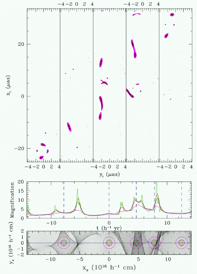
Figure 1: Caustics network (bottom panel), light curve (middle panel) and images relative to the source position (top panel) for a source trajectory that is parallel to the lens shear (the direction of x-axis). Different colors represent the 4 different source sizes.

Figure 1 and Figure 2 show the results for a source trajectory that is parallel to the shear direction. The bottom panel of Figure 1 shows the magnification pattern on the source plane, with a series of 4 concentric circles centered at 5 source positions; and the top panels show the images at these positions relative to the source (which has the same proper motion as the cloud). Different colors represent different source sizes. The middle panel of Figure 1 shows the light curves for the 4 source sizes with the blue dash lines used to mark the times for the five source positions. Figure 2 shows the “ray bundles” positions in the cloud frame at redshifts $1.69$, $0.83$, $0.57$, $0.1$. The 5 different columns show the 5 positions corresponding to those in Figure 1.

In the top row of Figure 2, one can see that the “ray bundles” at $z_{c}=1.69$, which is very close to the quasar, have almost exactly the same size and shape as the source and that the bundles show almost no bulk motion. The density of “ray bundles” clearly have the imprints from magnification pattern shown in the bottom panel of Figure 1. So if an absorption cloudlet has a similar or somewhat smaller size than a source that is sitting directly behind it, the depth of its corresponding absorption line will change dramatically as the source crosses the caustics. The magnification close to a fold caustic is proportional to the inverse square root of the distance from it, so for a cloud with angular size $\theta_{c}<\theta_{s}$, the fractional change in absorption line depth caused by the caustics scales as $(\theta_{c}/\theta_{s})^{3/4}$. Hence, for cloud close to the quasar redshift, structures on scale $\sim 10^{14}-10^{16}h^{-1}{\rm cm}$ (depending on the source size) will be probed over few-month to few-year timescales (i.e., the timescale of typical caustics crossings).

The fourth row of panels of Figure 2 shows “ray bundles” for $z_{c}=0.1$, which is close to the lens redshift. A distinct difference between these “ray bundles” from the ones at $z_{c}=1.69$ is that they are split into many groups of bundles, which correspond to the micro-images in the top panel of Figure 1. I dub these groups of “ray bundles” as micro-images in the following discussions. Most of these micro-images are stretched one-dimensionally, and most rays are concentrated in a few major micro-images. The micro-images in different columns have drastically different morphologies and positions. If there are cloudlets of similar sizes as these micro-images distributed on the cloud plane, then the absorption spectra will show multi-component absorption features at any given time. These components will experience drastic changes in line depth, with some components disappearing and other new components appearing during the course of months or years, as the source crosses the microlensing caustics. Another important characteristic is that the bulk of these micro-images are moving in the same direction as the source. This motion is described by equation (16), which yields $\sim 0.8\,h\,{\mu\rm as}\,{\rm yr}$. So from equation (14), structures as large as $\sim 3.0n\times 10^{16}\,h^{-1}\,{\rm cm}$ will be crossed in $n\times 10\,h^{-1}\,{\rm yr}$ by the bulk motion of the “ray bundles”. Hence, the effects caused by the micro-images and the bulk motion of the bundles together probe scales of $\sim 10^{14}-10^{16}h^{-1}{\rm cm}$ on timescales of months to years.

The second and third row of panels in Figure 2 refer to clouds at intermediate redshifts between the lens and the source. Their redshifts, $z_{c}=0.83$ and $z_{c}=0.57$, are close to the Mg II absorption systems observed by Rauch et al. (2002). As expected, the characteristics of these “ray bundles” are intermediate to those shown in rows 1 and 4. The overall shapes of the micro-images are close to that of the source, with magnification patterns imprinted on them. And they also clearly show multiple components, which appear and disappear as the source crosses caustics. The angular sizes of the images are close to that of the (unmagnified) quasar. These micro-images could probe clouds with angular size from a factor of few smaller to a factor of few larger than the source size, which corresponds to scales of $\sim 10^{14}-10^{16}h^{-1}{\rm cm}$. From equation (14) and (16), the bulk motion of the bundles will probe cloud structures $\sim 0.8n\times 10^{16}\,h^{-1}\,{\rm cm}$ and $\sim 1.3n\times 10^{16}\,h^{-1}\,{\rm cm}$ during $n\times 10\,h^{-1}\,{\rm yr}$ for $z_{c}=0.83$ and $z_{c}=0.57$, respectively.

For a source trajectory that is perpendicular to the shear, there will be almost no bulk motion relative to the cloud for the “ray bundles”, while the magnitude of bulk motions for intermediate trajectories is a fraction of the parallel case depending on their angles relative to the shear direction. And the micro-images of these trajectories share similar properties with those of the trajectory that is parallel to the shear. Figure 2 shows that micro-image motions are in the same orders as the bulk motion of macro-image over the timescales considered. Therefore, trajectory direction only has a modest impact on the cloud sizes probed.

These results are in great contrast with those of Brewer & Lewis (2005), who claimed quasar microlensing for image A of Q2237+0305 can induce considerable variability of absorption lines associated with structures as large as $0.1{\rm pc}$ during the course of years to decades. According to their analysis, the effect is largest when the cloud is very close to the source, and for example, the timescale of line strength variation for a $0.1{\rm pc}$ cloud very close to the source is given as $\sim 16.2{\rm yr}$. However, in their analysis, they effectively assumed the relative lens-cloud proper motion $\mu_{lc}=0$. This would lead to a timescale $t_{cc}\sim R_{c}D_{l}/({\rm v}_{l}D_{s})\sim 16(R_{c}/0.1{{\rm pc}}){\rm yr}$ for absorption cloud near the source redshift (they adopted ${\rm v}_{l}=600{\rm km}\,{\rm s}^{-1}$), which is in agreement with column 4 of their Table 1. In fact, I showed that, when peculiar velocities of the source and cloud are ignored, $\mbox{\boldmath$\mu$}_{lc}=\mbox{\boldmath$\mu$}_{ls}$ (eq. 15), which is not negligible. Even considering realistic peculiar motions of the source and the cloud, it still leads to time scales that are more than one order of magnitude slower than those predicted for $\mu_{lc}=0$. In addition, when the cloud is close to the source, the angular sizes of the clouds they considered are orders of magnitudes larger than their source size, so effects of changes in magnification pattern on the source plane alone have very little impact as well. Therefore, Brewer & Lewis (2005) significantly overestimated the cloud size to which microlensing is effectively sensitive.

4 Discussion and Conclusion

I have shown that there are two effects that might induce variation of absorption lines along the sight lines to lensed quasar. One effect is caused by the drastic morphological and positional changes of micro-images when the source crosses the caustic network. The other effect is due to the bulk motion of the “ray bundles” relative to the absorption clouds. I have laid out a basic framework in studying these effects for microlensed quasars in general. And in particular, I perform numerical simulations to apply the method to image A of Q2237+0305. I demonstrated that the combinations of these two effects probe $10^{14}-10^{16}\,h^{-1}\,{\rm cm}$ absorption cloudlets between the lens and the source over timescales of months to years. The existence of these cloudlets will be revealed by either changes in line depths or appearances/disappearances of multi-absorption components. Spectra should preferably be taken during the course of caustic crossings, which can be inferred from photometric monitoring programs of lensed quasars. In fact, the Mg II lines observed by Rauch et al. (2002) about 8 years ago already show different multi-components along sight lines of three different macro-images, implying they might be caused by fragmented cloudlets with similar sizes as the micro-images. A similar high-resolution spectrum taken in the near future would provide a definitive test of the existence for structures of Mg II or other metal-line absorbers at the scales of $10^{14}-10^{16}\,h^{-1}\,{\rm cm}$. If the spectral variations are indeed observed, a statistical study similar to Kochanek (2004) will be required to infer the properties of the cloudlets. Moreover, a time series of spectra may provide additional constraints to quasar microlensing models.

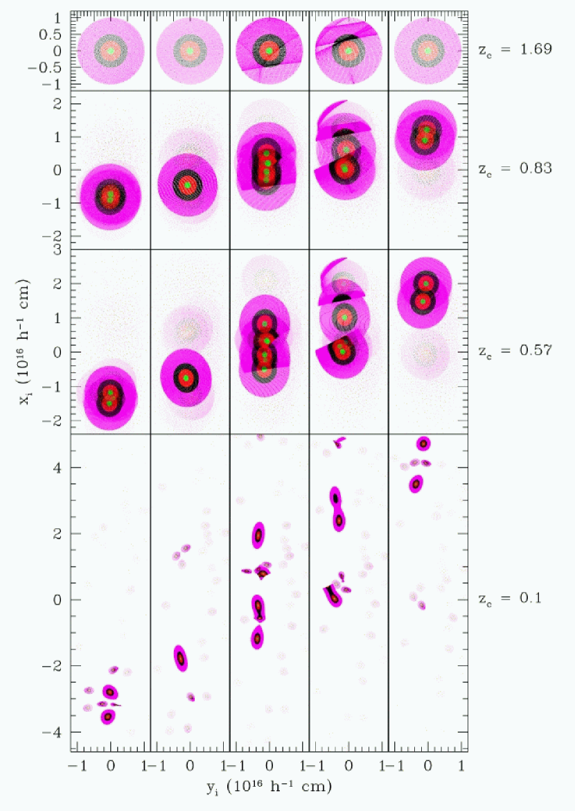
Figure 2: Physical positions of “ray bundles” in the frame of cloud at redshifts $0.1$, $0.57$, $0.83$ and $1.69$. The 5 different columns correspond to the source positions shown in Figure 1. x-axis is the direction of the lens shear.

References

- Brewer & Lewis (2005) Brewer, B. J., & Lewis, G. F. 2005, MNRAS, 356, 703
- Corrigan et al. (1991) Corrigan, R. T., et al. 1991, AJ, 102, 34
- Hao et al. (2006) Hao, H., et al. 2006, ApJL, submitted (astro-ph/0612409)
- Huchra et al. (1985) Huchra, J. et al. 1985, AJ, 90, 691
- Frank et al. (2006) Frank, S. et al. 2006, ArXiv Astrophysics e-prints, arXiv:astro-ph/0605676
- Kayser et al. (1986) Kayser, R. et al. 1986, A&A, 166, 36
- Kochanek et al. (1996) Kochanek, C. S. 1996, ApJ, 473, 610
- Kochanek (2004) Kochanek, C. S. 2004, ApJ, 605, 58
- Lanzetta et al. (1987) Lanzetta, K. M. et al. 1987, ApJ, 322, 739
- Mortonson et al. (2005) Mortonson, M. J. et al. 2005, ApJ, 628, 594
- Prochter et al. (2006) Prochter, G. E., et al. 2006, ApJ, 648, L93
- Rauch et al. (2002) Rauch, M. et al. 2002, ApJ, 576, 45
- Lewis & Ibata (1998) Lewis, G. F., & Ibata, R. A. 1998, ApJ, 501, 478
- Treyer & Wambsganss (2004) Treyer, M., & Wambsganss, J. 2004, A&A, 416, 19
- Wambsganss (1990) Wambsganss, J. 1990, Ph.D. Thesis
- Wambsganss (2006) Wambsganss, J. 2006, Saas-Fee Advanced Course 33: Gravitational Lensing: Strong, Weak and Micro, 453
- Woźniak et al. (2000) Woźniak, et al. 2000, ApJ, 529, 88
- Zibetti et al. (2005) Zibetti, S., et al. 2005, ApJ, 631, L105