The Monitor project: Data processing and lightcurve production

Abstract

We have begun a large-scale photometric survey of nearby open clusters and star-forming regions, the Monitor project, aiming to measure time-series photometry for $>10,000$ cluster members over $>10\ {\rm deg^{2}}$ of sky, to find low-mass eclipsing binary and planet systems. We describe the software pipeline we have developed for this project, showing that we can achieve peak RMS accuracy over the entire data-set of better than $\sim 2\ {\rm mmag}$ using aperture photometry, with RMS $<1\%$ over $\sim 4\ {\rm mag}$, in data from $2$ and $4\ {\rm m}$ class telescopes with wide-field mosaic cameras. We investigate the noise properties of our data, finding correlated ‘red’ noise at the $\sim 1-1.5\ {\rm mmag}$ level in bright stars, over transit-like timescales of $2.5\ {\rm hours}$. An important source of correlated noise in aperture photometry is image blending, which produces variations correlated with the seeing. We present a simple blend index based on fitting polynomials to these variations, and find that subtracting the fit from the data provides a method to reduce their amplitude, in lieu of using techniques such as point spread function fitting photometry which tackle their cause. Finally, we use the Sysrem algorithm to search for any further systematic effects.

1 Introduction

The Monitor project is a large-scale photometric survey of galactic open clusters and star forming regions. We intend to measure high-cadence time series photometry for $>10,000$ cluster members over $>10\ {\rm deg^{2}}$ of sky, aiming to find the first transiting planets in open clusters, and tens-hundreds of low-mass eclipsing binary systems, possibly including brown dwarfs. For more details of the project’s scientific goals and the results of simulations giving likely numbers of detected systems, the reader is referred to Aigrain et al. (2006), hereafter paper I. A brief summary of the project is also given in Hodgkin et al. (2006).

Data processing in this project is challenging. In a typical night we obtain $\sim 25\ {\rm Gigabytes}$ of imaging data using the Wide Field Camera (WFC) on the Isaac Newton Telescope (INT), and this can be as large as $\sim 50\ {\rm Gigabytes}$ for some of the other instruments we are using (for example MegaCam on the Canada-France-Hawaii Telescope, hereafter CFHT). Since our survey covers $9$ clusters over $>10$ nights per cluster, this is a multi-terabyte project.

Kjeldsen & Frandsen (1992) give a detailed discussion of differential photometry problems and techniques, from the point of view of attempting to detect low-amplitude stellar oscillations, but many of their arguments apply equally to transit surveys. Using CCD cameras, one can perform differential photometry on very large numbers of stars simultaneously, using non-variable stars in the field as comparison sources to remove transparency (and other) variations in the atmosphere. Differential photometric precision at the sub-$1\%$ level can be readily achieved using this method, even in somewhat non-photometric conditions.

Our methodology is based on experience gained by members of our group from the University of New South Wales Extrasolar Planet Survey (Hidas et al., 2005), and much of the pipeline code is now shared between the two projects.

We describe the observations in §2 and the basic CCD data reduction in §3. §4 gives an overview of the steps required to produce differential photometry, and hence lightcurves, from these data, and the practical details of their implementation are discussed in §5 and §6.

In §7 we examine the noise properties of our data, with particular attention given to correlated (‘red’) noise, which can be a serious problem in differential photometry (Pont, Zucker & Queloz, 2006). §8 examines one particular source of correlated noise, namely seeing-correlated variations induced in the lightcurves by blending of flux from neighbouring sources into the photometric apertures, and in §9 we apply the Sysrem algorithm (Tamuz, Mazeh & Zucker, 2005) to search for any further sources of correlated noise in the data. Finally, we summarise our conclusions in §10.

2 Observations

We are using wide-field mosaic cameras on several telescopes to perform the survey, principally: the Wide Field Camera (WFC) on the $2.5\ {\rm m}$ INT ($4\times$ 2k$\times$4k CCDs, $\sim 34\times 34^{\prime}$ field-of-view) and MegaCam on the $3.5\ {\rm m}$ CFHT ($36\times$ 2k$\times$4.5k CCDs, $\sim 1\times 1^{\circ}$ FoV) in the Northern hemisphere, and the ESO/MPG $2.2\ {\rm m}$ Wide Field Imager (WFI) ($8\times$ 2k$\times$4k CCDs, $\sim 34\times 33^{\prime}$ FoV) and Mosaic II on the $4\ {\rm m}$ CTIO Blanco telescope ($8\times$ 2k$\times$4k CCDs, $\sim 37\times 37^{\prime}$ FoV) in the Southern hemisphere. Due to the enormous quantity of data, a uniform strategy for observing (where possible) and data processing is essential.

The peculiarities of scheduling for each of these telescopes limit our flexibility in observing strategy so this will be discussed only briefly. We observe in $i^{\prime}$ or $I$, since this maximises signal-to-noise for our faint, red objects of interest, and minimises any colour-dependent atmospheric extinction, which can be difficult to correct in the lightcurves. The wide-field mosaic instruments we are using typically suffer from fringing in red bandpasses, so the SDSS-like $i^{\prime}$ filter (Fukugita et al., 1996) is preferred where available, since this minimises fringing due to its sharp red cut-off at $\sim 8500$ Å, compared to the long red tail of the standard $I$ filters.

Exposure times are selected to give good signal to noise on the largest possible number of cluster members, while keeping the targets sufficiently bright that medium-resolution follow-up observations on $4\ {\rm m}$ class telescopes and high-precision radial velocities on $8\ {\rm m}$ class telescopes remain feasible. Typically our exposures are in the range $30-120\ {\rm s}$, so the survey efficiency is overhead dominated with the slow readout times for the mosaic instruments we are using (most are $\sim 60\ {\rm s}$). In several cases we cycle between multiple fields in a single cluster to increase our spatial coverage, or between multiple clusters, but we aim to obtain an observing cadence no worse than $15\ {\rm minutes}$ for clusters where we are primarily searching for eclipsing binaries, and $5\ {\rm minutes}$ for planet searches, or where short-term stellar variability is a problem, ie. the youngest clusters (see paper I for more details).

Accurate flat fielding is of critical importance in differential photometry, so we take extra care to ensure that this is done as well as possible. We find that twilight flat fields provide superior results compared to dome flat fields for all the instruments we are using, provided sufficient signal can be accumulated. For a typical detector with gain of a few ${\rm e^{-}/ADU}$, and a typical twilight flat illumination level of $20,000\ {\rm ADU/pixel}=40,000\ {\rm e^{-}/pixel}$, the Poisson noise is $200\ {\rm e^{-}}$, ie. a signal-to-noise ratio of $200$, which is equivalent to $\sim 5\ {\rm mmag}$ photon noise per pixel. Averaged over a typical photometric aperture of $3\ {\rm pixel}$ radius this gives $\sim 1\ {\rm mmag}$ – ie. a significant contribution. Over a typical one week observing run, we can readily obtain at least $25$ flat field frames, which reduces the Poisson noise to $\sim 0.2\ {\rm mmag}$, a level which is perfectly acceptable for our purposes.

A related issue is that of positioning the telescope. Even using the flat fielding procedure described, small errors of the order of $0.1-1\%$ remain in the flat field frames, and fringing in the detectors, even after correction, can reach amplitudes of $\sim 0.2\ \%$. The effects can be divided into low spatial frequencies, dominated by non-uniform illumination of the flat field frame, and high spatial frequencies, eg. fringing, or differential variations in the quantum efficiency of the pixels (eg. as a function of wavelength, since the spectra of the flat field source and target star are different). The combination of these effects typically limits the achievable photometric precision to a few mmag depending on the instrument, in our experience. In order to minimise these effects we therefore aim to reposition each star on exactly the same pixel of the detector in each exposure. This is done by using the telescope guiding system to correct for pointing errors, where available. We note in passing that this procedure may introduce correlated noise (see §7), particularly in the event that any positioning errors are periodic or result in a slow drift across a few pixels of the detector. It has been suggested that an intentional random jitter in the telescope positions may prove beneficial to convert this source of correlated noise to a source of random noise. However, due to the need to move over a larger region of the detector, doing this is likely to introduce greater effects due to flat fielding errors, fringing, and other effects operating over short spatial scales. It therefore carries an inherent risk of raising the overall noise level, and thus would require more data, so we have been unable to explore it further as telescope time is always at a premium when using large international facilities.

Equatorial standard star fields (from the catalogue of Landolt 1992) are observed regularly during our observing runs, to provide calibrated photometry on a standard zero-point system.

3 Data reduction

The need for a uniform data processing strategy was highlighted in §2. We employ a modified version of the INT/WFC data reduction pipeline, developed for the INT Wide Field Survey (WFS) and originally described in Irwin & Lewis (2001). This has been successfully applied to data from all of the instruments mentioned in §2 at the time of writing.

Two of the instruments we are using (INT/WFC and CTIO Mosaic) suffer from electrical cross-talk between the detector readouts, the effect of which is illustrated in Figure 1. For the INT/WFC the maximum level is $\sim 4\times 10^{-4}$, typically a sufficiently low level to be ignored, but for the CTIO Mosaic the level is $\sim 2\times 10^{-3}$. Therefore, before starting the standard CCD reduction procedure this must be corrected, and is done in a simple manner by subtracting a fraction $f_{ij}$ of the detected counts on detector $i$ from detector $j$.

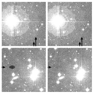
Figure 1: A section of CCDs 3 (top) and 4 (bottom) of an INT/WFC image of M34, before (left) and after (right) applying the cross-talk correction described in the text. The images show positive cross-talk ($f_{ij}>0$) from CCD 4 to CCD 3 (eg. at the position in the top panel corresponding to the pair of bright stars visible at the right of the bottom panel, marked with arrows), and negative cross-talk ($f_{ij}<0$) from CCD 3 to CCD 4 (eg. at the position in the bottom panel corresponding to the brightest star on the left hand side of the top panel, marked with an arrow).

We then follow the standard CCD reduction scheme of bias correction, trimming of overscan and non-illuminated regions, non-linearity correction, flatfielding and gain correction, followed by defringing, catalogue generation, astrometric and photometric calibration described in Irwin & Lewis (2001). We use the point source catalogue (PSC) from the Two-Micron All Sky Survey (2MASS) as an astrometric reference catalogue, which we find gives typical RMS residuals of $<0.1^{\prime\prime}$.

4 Differential photometry

In the discussion that follows, we use aperture photometry. The technique we use is similar to standard aperture photometry, except our apertures are ‘soft-edged’, and overlapping sources are fitted simultaneously using circular top-hat functions as the ‘PSF’. We have found that for our open cluster fields, this technique is sufficient to obtain a photometric precision of $\sim 1-2\ {\rm mmag}$ for the brightest stars, without need to invoke more exotic techniques such as point spread function fitting (PSF-fitting; eg. Stetson 1987) or difference image analysis (DIA; Alard & Lupton 1998, Alard 2000), although these are discussed briefly in §8.

4.1 Background estimation

Robust, repeatable background estimation is of vital importance in aperture photometry. We use a variant of the technique discussed in Irwin (1985) for background estimation in our aperture photometry, which has been found empirically to work at least as well as the standard technique of using an annulus around the photometric aperture, for fields with slowly-varying sky backgrounds. A brief description of the method is given here, and the reader is referred to Irwin (1985), Irwin (1996) and Irwin et al. (in prep) for a more detailed discussion.

Briefly, the image is divided into a coarse grid of $64\times 64\ {\rm pixel}$ bins ($\sim 20\ {\rm arcsec}$ on sky). The background level in each bin is estimated using a robust $k\sigma$ clipped median of the counts in that bin, using the robust median of absolute deviations (MAD; eg. Hoaglin et al. 1983) estimator to calculate $\sigma$, and rejecting bad pixels using the confidence maps (see Irwin & Lewis 2001). The resulting map is filtered using 2-D bilinear and median filters to avoid problems due to single bins dominated by bright stars. The background in a given image pixel can then be estimated using bilinear interpolation over the coarse background map.

4.2 Aperture placement

Differential photometry is very sensitive to small positioning errors when placing photometric apertures on the science images. For a Gaussian PSF, the error in the derived fluxes is given to first order by:

$${\delta F\over{F}}\approx{1\over{\sqrt{2\pi}}}\ {\delta x\over{\sigma}}\ {2r\delta x\over{\sigma^{2}}}\ {\rm e}^{-r^{2}/2\sigma^{2}}$$ (1)

where $\delta x$ is the positioning error, $r$ is the radius of the aperture, and $\sigma$ describes the PSF size (ie. seeing, ${\rm FWHM}\approx 2.35\sigma$). See Appendix A for a derivation.

Typically we set $r=2.35\sigma$, ie. an aperture radius equal to the image FWHM, so:

$${\delta F\over{F}}\sim 0.119\ {\delta x^{2}\over{\sigma^{2}}}$$ (2)

Taking for example a typical value $\delta x=0.1\sigma$, this implies a flux error of $\approx 1\ {\rm mmag}$. Eq. (1) also confirms the intuitive result that using a larger aperture reduces the effect of centroid errors, at the cost of increased noise from the sky background.

We therefore first consider the question of how best to determine the correct locations for the apertures.

The ‘default’ technique used by existing source extraction software, as included in our pipeline (Irwin 1985, Irwin & Lewis 2001), or SExtractor (Bertin & Arnouts, 1996), is to find the centroid of each star on the CCD frame in question, to place an aperture at this position, and measure the flux. The accuracy to which this can be done for a star measured with signal to noise ratio $S$ improves in proportion to $1/S$ (eg. Irwin 1985), giving the general ‘rule of thumb’ that the error in the image centroid is $\Delta x/S$ where $\Delta x$ is the sampling interval (pixel scale), implying in general a decrease in the accuracy of aperture placement moving to fainter stars.

A further problem is that as the seeing changes, the amount of blending in very close sources will also vary, to the point that they could become resolved in frames with good seeing, and unresolved in frames with poor seeing. This causes the centroid to shift in the unresolved (or poorer seeing) image toward the companion star, and hence results in a serious error in the aperture flux measurements.

The standard method for solving these problems, which we call ‘co-located aperture photometry’, is therefore to use as many stars as possible to determine the aperture positions, in two stages. The first is to determine accurately the relative centroid positions of all the stars on the frame, which will be the same for all frames in the time-series (provided the stars do not move). This can be done using a stacked image to increase $S$ (we typically stack the $20$ frames with the best seeing, providing a $\sim$ four-fold improvement in $S$ over a single frame) and thus obtain an improved master catalogue with more accurate relative positions. Furthermore, since the placement of the apertures remains consistent, the effects of varying seeing are limited purely to varying flux loss from the apertures, which can be corrected to a good approximation by a global normalisation over the frame.

In the second stage, a transformation is computed between this master frame and each frame in the time-series on a per-detector basis, using a standard 6-coefficient linear transformation, derived using a least-squares fit to a large number of bright stars. In this case, the error for the bright stars is dominated by the error in the transformation, and assuming sufficiently large numbers of stars were used, this is in turn dominated by errors in the model, eg. due to radial distortions or other similar effects. Moreover, any errors in the mapping from the master frame to the individual frames will typically either affect all stars in the same way, or will be a smoothly-varying function of position. Such effects are readily removed using a simple polynomial fit (see §4.4).

Figure 2 illustrates this for our M50 data. In this case we have used a simple constant multiplier to normalise each frame to the photometric system of the master frame, using an iterative $k\sigma$ clipped fit (derived from the objects classified as stellar) to remove any variable stars. In Monitor data, although there is little to no improvement using the ‘co-located apertures’ technique for the majority of sources, it is still necessary to eliminate the problem of centroid shifts in blended sources, as we have suggested. We suspect that this is the origin of the spurious variable sources seen in the upper panel of Figure 2. Furthermore, another advantage is clear at the faint end, where it provides much more complete sampling, since we can still place an aperture and measure the flux even if the object does not pass the detection threshold on that particular frame, whereas in the upper panel, the object must be detected and the centroid computed before this can be done.

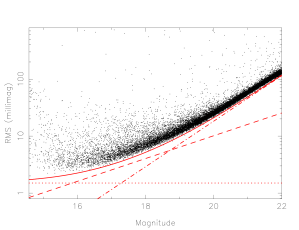
Figure 2: Plots of RMS scatter as a function of magnitude for the $i^{\prime}$-band observations of M50, showing all objects of stellar morphological classification. The upper plot shows the results obtained by placing the photometric apertures at the centroid positions of the stars, as determined on each frame, and the lower plot shows the same using the ‘co-located apertures’ technique. The plots have been truncated at $i^{\prime}\sim 22$ since we require the sources to be detected in at least $10\%$ of the images for the upper diagram, and the detections start to become substantially incomplete for fainter magnitudes. In both cases, a simple zero point correction of the individual frames to the master frame has been used (see §4.4). The diagonal dashed lines show the expected RMS from Poisson noise the object, the diagonal dot-dashed lines show the RMS from sky noise in the photometric aperture, and the dotted lines show an additional $1.5\ {\rm mmag}$ contribution added in quadrature to account for presumed systematic effects. The solid lines show the overall predicted RMS, combining these contributions.

For under-sampled data, the required fractional accuracy relative to the pixel scale is much more stringent, and the noise-induced centroid errors alone can become highly significant, eg. giving a $\sim 50\%$ improvement in RMS scatter for significantly under-sampled data from the University of New South Wales extrasolar planet search (Hidas et al., 2005).

4.3 Aperture sizes

It is straightforward to show that for the majority of images, an aperture with radius approximately equal to the FWHM of the stellar images achieves the optimal balance between flux loss (and consequently, increased Poisson noise in the counts) and integrated noise in the sky background (which increases with the area of the aperture). However, for bright sources, this wastes flux since the relative size of the sky noise contribution is much smaller, and a much larger aperture can be used.

Our aperture photometry procedure computes the flux in a sequence of apertures of radii $r_{\rm core}$, $\sqrt{2}\ r_{\rm core}$, $2\ r_{\rm core}$, etc. (doubling the area each time) where the ‘core radius’ $r_{\rm core}$ is set equal to the typical FWHM of stellar images (and kept fixed for all the data). We use $r_{\rm core}=4\ {\rm pixels}$ ($\sim 1.1\ {\rm arcsec}$) for the CTIO-4m+Mosaic data.

We employ a simple procedure to make use of these measurements. The lightcurve is computed for each aperture separately, and the root mean square scatter (computed using a robust median-based estimator) compared for each source. We simply choose the aperture with the smallest RMS for that star. This procedure ensures that larger apertures are used where they give an improvement for bright sources, but also accounts for blending, where using a larger aperture results in increased contamination of the flux measurement by neighbouring stars, and introduces modulations into the lightcurve as the seeing (and hence the amount of contaminating flux in the aperture) changes.

In order to place all the stars onto the same zero point system, this procedure necessitates using aperture corrections, to account for the differing amounts of flux lost from the different sized apertures. These are computed as simple ratios of the flux measured in the different apertures, for non-variable stars.

The dominant effect of this procedure is to produce a small improvement in the achieved RMS scatter for the bright stars in the sample. Figure 3 shows a comparison between the results of using this procedure, and using only the $r_{\rm core}$ (smallest) aperture. We have used a simple constant multiplier to normalise each frame to the photometric system of the master frame, via an iterative $k\sigma$ clipped fit to remove any variable stars.

Figure 3: Plots of RMS scatter as a function of magnitude for the $i^{\prime}$-band observations of M50, showing all objects of stellar morphological classification. The upper plot shows the results obtained using a single photometric aperture (radius $r_{\rm core}=4\ {\rm pixels}$), and the lower plot shows the same using multiple apertures, selected on a per-star basis. Lines as Figure 2. In both cases, a simple zero point correction of the individual frames to the master frame has been used (see §4.4).

4.4 Normalisation

The dominant effect of the atmosphere in ground-based differential photometry is a time-variable shift in the photometric zero point of each frame in the time-series. This can result from the combination of several effects, and is dominated by variations in transparency and overall extinction (including the airmass-induced change in the extinction seen on the frame). Nightly zero point correction using photometric standard star fields, as is commonly done for measuring absolute photometry, is sufficient to reach the level of a few percent down to $\sim 1\%$. Considerable progress can be made for the purposes of differential photometry, especially over small fields of view, by using non-variable stars in the field of interest to compute zero point shifts for each frame in the time-series.

For wide-field instruments such as the ones we are using, higher-order effects start to become significant. In particular, over a $\sim 0.8\ {\rm deg}$ diameter field (eg. INT+WFC or CTIO+Mosaic from corner-to-corner), differential variations in airmass across the frame are no longer negligible. Assuming the approximation for the airmass

$$X\approx\sec\zeta$$ (3)

where $\zeta$ is the zenith distance, and differentiating,

$${\delta X\over{X}}={\tan\zeta}\ {\delta\zeta}$$ (4)

Substituting a typical value of $\zeta=30^{\circ}$, $\delta X\approx 0.009$. For a typical $V$-band atmospheric extinction of $0.1\ {\rm mag\ airmass^{-1}}$, this contribution is $\sim 0.9\ {\rm mmag}$, and becomes larger moving away from the zenith. Figure 4 shows the difference in extinction across a $0.8\ {\rm deg}$ field as a function of zenith distance.

Figure 4: Differential extinction across a $0.8\ {\rm deg}$ field as a function of zenith distance, for an assumed atmospheric extinction of $0.1\ {\rm mag\ airmass^{-1}}$.

Since there are other slowly-varying effects as a function of position on the frame (eg. some flatfielding problems, astrometric errors inducing position-dependent loss of flux from the apertures, etc.) we have opted for a generalised approach of fitting 2-D polynomials to the magnitude residuals for each non-variable reference star on each frame, rather than enforcing the particular airmass dependence for atmospheric extinction (and in our experience this technique does indeed give better results). We have found a quadratic of the form:

$$\Delta m(x,y)=c_{0}+c_{1}x+c_{2}y+c_{3}xy+c_{4}x^{2}+c_{5}y^{2}$$ (5)

to be sufficient for all our wide-field data thus far, where $x$ and $y$ are the pixel coordinates (with the means $\bar{x}$ and $\bar{y}$ subtracted to give a zero-mean coordinate system, which improves the stability of the least-squares solution), $c_{i}$ are the polynomial coefficients (fit for each frame from a number of non-variable reference stars) and $\Delta m(x,y)$ is the zero point offset at the position $x,y$ on the frame.

Non-variable stars can be identified automatically by using the RMS of the lightcurves to reject any variable sources. We have found that it is often possible to compute this directly from the uncorrected light curve to obtain the initial fit of (5), and the refine the solution iteratively by rejecting the most variable stars at each stage. This technique selects $\geq 100$ non-variable bright stars on each CCD of the mosaic for the Monitor data.

Figure 5 compares the effects of applying no zero point correction, a simple zero point shift, and the full quadratic fit, for our CTIO-4m+Mosaic M50 data. The best precision reached was $\sim 35\ {\rm mmag}$ for the first case, $3\ {\rm mmag}$ with the zero point shifts, and $2\ {\rm mmag}$ with the quadratic fit.

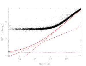
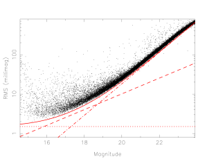
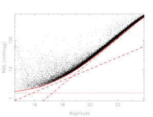
Figure 5: Plots of RMS scatter as a function of magnitude for the $i^{\prime}$-band observations of M50, showing all objects of stellar morphological classification. The upper plot shows the results with no zero point correction, the centre plot the effect of applying the zero-order correction only, and the lower plot shows the full quadratic correction. Lines as Figure 2.

4.5 Atmospheric scintillation

Scintillation provides a fundamental limit to the noise performance which can be reached in ground-based photometry. Conventional results for the scintillation level have typically assumed that one star is observed at a time, and we might expect that some of the scintillation would be cancelled out in CCD photometry due to the availability of simultaneous observations of comparison stars. However, Ryan & Sandler (1998) show that the typical coherence length is $\sim 12\ {\rm arcsec}$, so over the fields of view we are considering, the single star result should apply to a good approximation. Therefore, we can adopt the usual expression (see Ryan & Sandler 1998) of:

$${\sigma_{\rm scint}\over{F}}\approx 0.09{X^{3/2}\over{D^{2/3}\sqrt{2T}}}\ \exp\left(-{h\over{h_{0}}}\right)$$ (6)

where $\sigma_{\rm scint}$ is the RMS scintillation (in flux units), $F$ is the object flux, $X$ is the airmass, $D$ is the telescope aperture in centimetres, $T$ is the exposure time in seconds, $h$ is the telescope altitude, and $h_{0}$ is a turbulence weighted atmospheric altitude, taken here to be $h_{0}=8\ {\rm km}$. For the INT+WFC survey $i$-band observations this value is $0.44\ {\rm mmag}$, and for CTIO+Mosaic $0.21\ {\rm mmag}$. In both cases, scintillation is negligible compared to the dominant noise sources in the data. This is nearly always the case for moderate exposure times on large telescopes.

5 Implementation details

We present here some details of our actual implementation, as based on the discussion in §4, for completeness.

The frame-to-frame astrometric transformations are computed using a full astrometric model including radial distortions, by performing an internal astrometric refinement. A single data frame, typically the one taken in best seeing and sky conditions, with a good absolute astrometric solution (against 2MASS), is used as a reference. The pipeline-generated object catalogue for this frame is used to produce an astrometric reference catalogue, using the measured positions for all bright, stellar sources (we use sources down to $2\ {\rm mag}$ below saturation). The astrometric solution for each data frame in the field is then refined against this reference. The internal accuracy after this procedure is typically $1/10\ {\rm pixel}$ or better.

We generate the master catalogue by stacking the $20$ data frames taken in the best seeing and sky conditions, and use the standard pipeline source detection and morphological classification software. The classification software (see Irwin et al. in prep for a more detailed description) uses the flux of each object, measured in a series of apertures of increasing radii: $r_{\rm core}/2$, $r_{\rm core}$, $\sqrt{2}\ r_{\rm core}$, $2\ r_{\rm core}$ and $2\sqrt{2}\ r_{\rm core}$, where the default $r_{\rm core}$ is set approximately equal to the FWHM of the stellar images. By comparing these flux measures (including also the peak height), the locus of stellar objects (which all have approximately the same PSF and hence the same flux ratios between apertures) is defined in planes of flux ratio as a function of magnitude formed from several combinations of the measures. This is used to define a mean and standard deviation of the flux ratio for the stars, as a function of magnitude, and a normalised statistic is generated from this measuring how ‘stellar-like’ each image is. A classification flag is subsequently derived by defining a boundary in the statistic, and also factoring in the measured image ellipticities.

6 Lightcurve production

We use a simple procedure for lightcurve production. The first stage is to convert all the flux measurements to magnitudes. All of the remaining stages of the processing are performed in magnitudes rather than flux units for convenience. Points with null or negative fluxes (ie. below sky) are excluded from the lightcurves. Each CCD of the mosaic is processed separately (there are always enough stars to do this in our fields of interest, otherwise we would have to use another procedure).

The median and RMS flux of each object is calculated over all the differential photometry measurements, using a robust MAD estimator scaled to the equivalent Gaussian standard deviation (ie. $\sigma\approx 1.48\times{\rm MAD}$). We apply the procedure of §4.4 to fit and subtract a 2-D quadratic surface from the residuals as a function of $x$ and $y$ coordinates on each frame. In order to reduce contamination, the 2-D surface fits use inverse variance weighting (using the RMS flux of each object calculated earlier), and we exclude objects flagged as possible blends, saturated datapoints, and all objects with non-stellar morphological classifications.

We estimate expected per-datapoint photometric errors as the quadrature sum of components from Poisson noise in the object counts, Poisson noise in the sky, RMS of the sky background fit (multiplied by the square root of the number of pixels in the aperture), and a constant component of $\sim 1.5\ {\rm mmag}$ (as in Figure 5, for example) to account for systematic errors. See §7 for a more detailed analysis of this last component.

The lightcurves for each field are written into FITS binary tables in multi-extension FITS files, with one extension per detector (this convention is also used for the images, object catalogues and differential photometry output). These tables have one row per input object from the master catalogue, and the lightcurve itself, the photometric error on each lightcurve point and the heliocentric Julian date of observation, are stored in columns of the table. Our lightcurve generation software, and this file format, have been specifically designed to efficiently handle very large data-sets, for example we have also successfully used them on data from the SuperWASP transit search project (Pollacco et al., 2006).

At this stage, the data are ready for lightcurve analysis. Our analysis software, including period finding algorithms, an implementation of the transit search algorithm of Aigrain & Irwin (2004) and a number of other programs, interface directly to the lightcurve FITS files, and write their results out to additional columns in the files for convenient storage.

Typically the full reduction of one week of data from the INT+WFC or CTIO-4m+Mosaic takes $\sim 3\ {\rm days}$ including manual checking of the pipeline results. Often the most time-consuming stage of the entire process is reading the data onto disk, which ranges from relatively fast ($\sim 1\ {\rm day}$) using external IEE-1394 hard disks (eg. for ESO WFI data), to very slow (up to $1\ {\rm week}$) for DLT tapes. We stress the increasing importance of this issue as data rates from astronomical facilities continue to increase, and the enormous savings in time and cost afforded by using internet transfers (where possible) or efficient media such as external hard disks or LTO-2 tapes.

7 Noise properties

Lightcurves from ground-based transit surveys are invariably found to show significant correlated, or ‘red’ noise (see Pont et al. 2006 for a very detailed discussion). These correlations mean that, averaging over $N$ data points, the error in the mean drops less quickly than the ‘white’ (uncorrelated) noise prediction:

$$\sigma_{N}=\sigma_{0}/\sqrt{N}$$ (7)

where $\sigma_{N}$ is the error in the mean of $N$ data points, and $\sigma_{0}$ is the error in a single data point (where we have assumed, for simplicity, that the uncertainties are equal for all the data points). Throughout this analysis, we assume a value of $N$ corresponding to $\sim 2.5\ {\rm hours}$, an appropriate timescale for a hot Jupiter transiting a solar-like star, but also comparable to timescales for eclipses in low-mass EBs. We have tried to maintain consistent notation with Pont et al. (2006) throughout this Section.

The least-squares problem of finding the best-fitting box-shaped transit model for a given lightcurve reduces to simply finding the inverse variance weighted mean of the in-transit data points (eg. Aigrain & Irwin 2004), giving the transit depth if the mean of the out-of-transit data points is subtracted. In order to evaluate the significance of a given detection, we use the detection statistic $Q$ of Aigrain & Irwin (2004), repeated here:

$$Q=\left(\sum_{i=1}^{N}{d_{i}\over{\sigma_{i}^{2}}}\right)^{2}\left(\sum_{i=1}^{N}{1\over{\sigma_{i}^{2}}}\right)^{-1}$$ (8)

where the summations run over all in-transit data-points $i$, $d_{i}=f_{i}-\bar{f}$, the difference between the $i$th measured flux $f_{i}$ and the average flux $\bar{f}$ over all measurements, and $\sigma_{i}$ is the uncertainty on the $i$th flux measurement.

The presence of correlated noise in the lightcurves tends to give larger values of $Q$ in the absence of transits. Consequently, to maintain a low false alarm rate, we must use a higher detection threshold in $Q$, reducing sensitivity to shallow transits, or those with few in-transit data points. Furthermore, if the level of correlated noise in each lightcurve is known, Eq. (8) can be modified to account for this in the transit detection process (see Pont et al. 2006).

We have examined the noise properties of our data using a method based on that of Pont et al. (2006). We present results based on the M50 lightcurves as a ‘best case’ where we believe that our data reduction is closest to optimal. It should be noted that the prescription we follow for evaluation of red noise will not work at very faint magnitudes, where random noise sources dominate over the correlated noise. We have therefore analysed lightcurves of the brightest non-saturated stars in our sample, where the effects of red noise are much more significant.

Figure 6 shows the RMS scatter as a function of magnitude for a sample of lightcurves chosen to be approximately ‘flat’ (small reduced $\chi^{2}$), which should be noise-dominated. We have calculated $\sigma_{0}$ and $\sigma_{N}$ from (7) for $N=19$, corresponding to $2.5\ {\rm hours}$ with the sampling of these data, and compared $\sigma_{N}$ with $\sigma_{2.5}$ calculated as the RMS of means over a $2.5\ {\rm hour}$ window moved along the lightcurve. This measures the correlated noise over a transit-length window, and in general is larger than $\sigma_{N}$ if there are correlations on this time-scale. The results indicate that the level of correlated noise on these time-scales is $\sim 1-1.5\ {\rm mmag}$ at the bright end. Other teams have found instances of an increase in the level of correlated noise at faint magnitudes, and Figure 6 shows that the same is true here for the majority of the stars, where the $\sigma_{2.5}$ values never converge to the $\sigma_{N}$ values. Two likely causes of such effects are residuals in the sky background determinations, and blending, both of which are likely to affect faint stars close to sky more than bright stars.

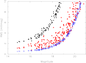
Figure 6: Lightcurve RMS as a function of magnitude for a subset of M50 lightcurves not flagged as blended. The symbols indicate the three RMS measures: filled circles are values of $\sigma_{0}$, the RMS scatter per data point, filled triangles are $\sigma_{2.5}$, the RMS scatter of averages over $2.5\ {\rm hour}$ windows, and asterisks are $\sigma_{N}$, the predicted RMS scatter over the $2.5\ {\rm hour}$ window assuming white noise. The filled triangles lie between the other symbols, indicating the presence of correlated noise at the $\sim 1-1.5\ {\rm mmag}$ level over $2.5\ {\rm hours}$ for the brightest stars, where the correlations dominate over random (white) photometric noise.

In order to make a quantitative estimate of the level of correlations in the noise, we have attempted to measure how rapidly the noise ‘averages out’ as a function of the number of data points observed in-transit. Figure 7 shows the result for a single ‘flat’ lightcurve at the bright end of the RMS diagram ($I\sim 15$). In order to generate the diagram, a $\sim 2.5\ {\rm hour}$ window was moved over the data in $2\ {\rm minute}$ time intervals (approximately $1/4$ of the sampling), counting the number $n$ of data points lying in the interval, and recording the mean of the data points. We then computed $V(n)$ as the variance of the means at each value of $n$ (where more than one mean was available). For uncorrelated (white) noise we expect $V(n)=\sigma_{w}^{2}/n$, where $\sigma_{w}$ is the standard deviation of the white noise. In general there is an additional red noise component, which does not average out as the number of data points is increased, ie.

$$V(n)=\sigma_{r}^{2}+{\sigma_{w}^{2}\over{n}}$$ (9)

where $\sigma_{r}$ is the standard deviation of the red noise component.

Figure 7: The square root of $V(n)$ (ie. the standard deviation) plotted for a single ‘flat’ lightcurve, with $\sigma_{0}=2.5\ {\rm mmag}$, $\sigma_{2.5}=1.3\ {\rm mmag}$, and $\sigma_{N}=0.6\ {\rm mmag}$. The solid line shows the white noise prediction $V(n)=\sigma_{w}^{2}/n$, and the dashed line shows the fit of Eq. (9) to the data, with parameters $\sigma_{w}=3.8\ {\rm mmag}$ and $\sigma_{r}=1.3\ {\rm mmag}$. The scatter (especially at large $n$) is caused by the limited number of $2.5\ {\rm hour}$ windows in the lightcurve containing these particular numbers $n$ of data points. The dot-dashed line shows the predicted curve derived from the autocorrelation function of this lightcurve, using Eq. (11).

Figure 8 shows the values of $\sigma_{r}$ as a function of magnitude for all the lightcurves in Figure 6. The upper envelope of derived values increases toward the faint end, ie. the red noise level is higher at faint magnitudes, as discussed earlier. We note that the increased random noise level at the faint end affects the determination of the values of $\sigma_{r}$ (and $\sigma_{0}$), and hence introduces scatter as seen in Figure 8.

Figure 8: Values of $\sigma_{r}$ from fitting Eq. (9) plotted as a function of magnitude. The upper envelope of derived values increases toward the faint end, which suggests that the red noise level increases for fainter stars.

An alternative method to investigate correlations among the time-sampled data points is to compute the autocorrelation function. Figure 9 shows the autocorrelation function $\phi(\tau)$ of a representative ‘flat’ M50 lightcurve, defined as:

$$\phi(\tau)=\sum_{n=1}^{N}\sum_{i=1}^{P_{n}}(m_{i,n}-\bar{m_{n}})(m_{i+\tau,n}-\bar{m_{n}})$$ (10)

where the outer sum is over nights of data $n$, and the inner sum over data points within the night, up to the total $P_{n}$ taken in that night. $m_{i,n}$ is the magnitude of the star in measurement $i$ of night $n$, and $\bar{m_{n}}$ is the mean magnitude of the star in night $n$. The summations were performed in this manner to avoid the nightly gaps influencing the results for short time-scales.

The results indicate that the characteristic coherence timescale of the correlations we see is $\sim 30\ {\rm minutes}$ (or $6$ data points), which is typical of the ‘flat’ lightcurves in the M50 data-set.

Figure 9: Autocorrelation function of a ‘flat’ M50 lightcurve, normalised to the zero-lag value ($\tau=0$). The sampling is approximately one data point every $6$ minutes, and the level of correlation is negligible for $\tau>6\ {\rm datapoints}$.

It is straightforward to show that the expected $V(n)$ can be expressed in terms of the autocorrelation function as:

$$V(n)={\sigma_{w}^{2}\over{n}}\left[1+2\sum_{k=1}^{n-1}{n-k\over{n}}\ \phi(k)\right]$$ (11)

This function is shown as the dot-dashed line Figure 7, for an example lightcurve from the M50 data-set, and provides a better approximation to the observed functional form for $n\la 10$ than the simple single-parameter description of Eq. (9). Note that Eq. (11) is not expected to exactly reproduce the calculated $V(n)$ because for a given value of $n$, $V(n)$ counts only 2.5 hour windows containing $n$ data points, ie. for small $n$ the function is dominated by the behaviour at the end of the night, or at the end of observing windows interrupted by the weather, whereas the ACF calculates the correlated noise over the entire lightcurve for all $n$.

We find overall levels of ‘red noise’ at the low end of the range spanned by other surveys (eg. see Pont et al. 2006, Smith et al. 2006), of $\sim 1.5\ {\rm mmag}$ at the bright end. Since telescope time is at a premium, we have only been able to use one observing strategy throughout, so it is difficult to quantify the factors contributing to $\sigma_{r}$ from the present data-set. However, since our levels of red noise are comparable to the existing ground-based surveys, we suggest that we may be obtaining close to the best achievable performance for a ground-based survey over a $\sim 40\ {\rm arcmin}$ field using $2-4\ {\rm m}$ class telescopes, and that the strategy of trying to keep the positions of the sources on the detector as close as possible to constant, appears to be successful. Nevertheless, it would be interesting to investigate the possibility of using small random offsets to attempt to randomise the noise.

8 Seeing-correlated effects

We performed a search for correlations in the lightcurves with a number of external parameters, including the image FWHM, sky level (both globally and local to the sources), airmass, hour angle and image morphology (major axis, ellipticity, position angle). The dominant effect was found to be seeing-correlated variations induced by image blending.

Variations in the seeing cause an increase in the amount of blended flux in the photometric apertures as the FWHM of the stellar images increases, so therefore we expect to find a correlation between the measured FWHM and the magnitude, for lightcurves of blended objects. This can be used both for flagging blended objects, and as we shall see, for removing some of the variations induced by blending.

Our source detection software flags any objects where the deblending algorithm (eg. Irwin 1985) was invoked, and this flag is propagated into the lightcurves to assist with identifying blended objects. We have found empirically that the flag is often set for objects which do not exhibit any obvious blending effects in the lightcurves, since a greater degree of overlap is required before the object lightcurve becomes sufficiently contaminated.

We therefore developed an empirical technique to characterise the level of blending-induced effects in each lightcurve, by looking for seeing-correlated shifts of the object from its median magnitude. This is done by fitting a simple quadratic polynomial to the shift as a function of the measured FWHM of the stellar images on the corresponding frame. Some examples are shown in Figures 11 and 12. We use the following statistic to quantify the level of blending:

$$b={\chi^{2}-\chi_{\rm fit}^{2}\over{\chi^{2}}}$$ (12)

where $\chi^{2}$ is defined as

$$\chi^{2}=\sum_{i}{\left(\sum m_{i}-\bar{m}\right)^{2}\over{\sigma_{i}^{2}}}$$ (13)

for lightcurve points $m_{i}$ with uncertainties $\sigma_{i}$, and $\bar{m}$ is the median magnitude in the lightcurve. $\chi^{2}_{\rm fit}$ is the same statistic measured with respect to the quadratic model. $b>0$ implies that $\chi^{2}$ was improved by the model fit – ie. increasing values of $b$ to the maximum $b=1$ imply progressively greater amounts of seeing correlation in the lightcurve, or increasing levels of blending.

Figure 10 shows a histogram of the blend index, indicating the presence of a peak at $b\sim 0.8$, corresponding to objects showing clear seeing-correlated features due to blending, and another peak at $b\sim 0$ corresponding to lightcurves without seeing correlations. The deblending flag from the source detection software appears to work well for selecting lightcurves with no blending, and hence no seeing correlation, but also flags relatively large number of objects showing little or no seeing-correlated behaviour, due to varying degrees of overlap.

Figure 10: Histogram of the blend index $b$ for all lightcurves of stellar morphological classification in the CTIO M50 data. The solid line includes all objects, and the dashed line only those objects flagged as blended by the source detection software. The lower panel shows an expanded version of the upper panel.

A natural progression from the analysis we have described is to attempt to remove some of the seeing-correlated features in the lightcurves by subtracting the fit. Figures 11 and 12 show the results of doing this for two typical lightcurves: one showing significant seeing correlated behaviour ($b=0.78$) and the other showing little seeing correlated behaviour ($b=0.16$). In both cases, the procedure significantly reduces the amount of seeing correlated features, and importantly, does not introduce significant additional correlated features. In both cases the lightcurve RMS was reduced, as expected. Figures 13 and 14 show that this corresponds to a reduction in the level of correlated noise as measured in §7. We have used this simple approach to produce a filter which can be optionally applied to our lightcurves before embarking on transit searches and other similar analyses.

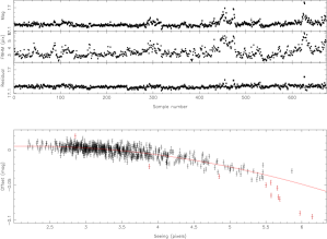
Figure 11: Example of a lightcurve showing seeing correlations from our CTIO M50 data. The upper three panels show (from top to bottom) the lightcurve, the seeing, and the residual after subtracting the quadratic fit. The lower panel shows the polynomial fit (solid line), and the data plotted as error bars (points coloured red were excluded by the iterative fitting procedure). The statistic $b=0.78$ for this lightcurve, and the RMS was reduced from $7.2\ {\rm mmag}$ to $5.3\ {\rm mmag}$ after subtracting the fit. In this case the results could be improved further by using a higher degree for the polynomial (eg. a quartic).

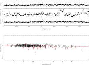
Figure 12: Example of a lightcurve showing weak seeing correlations from our CTIO M50 data. Panels as Figure 11. The statistic $b=0.16$ for this lightcurve, and the RMS was reduced from $3.6\ {\rm mmag}$ to $3.5\ {\rm mmag}$ after subtracting the fit.

Figure 13: Plots as Figure 7 for the object in Figure 11 before (top) and after (bottom) subtracting the polynomial fit. The value of $\sigma_{r}$ changed from $9.4$ to $3.8\ {\rm mmag}$, and $\sigma_{w}$ from $8.1$ to $5.0\ {\rm mmag}$, indicating a significant reduction in the levels of white and correlated noise for this lightcurve.

Figure 14: Histograms of $\sigma_{2.5}$, the RMS scatter of averages over $2.5\ {\rm hour}$ windows, for all lightcurves flagged as possible blends on a single detector in the M50 data-set, before (dashed line) and after (solid line) the correction for seeing-correlated lightcurve features, showing the reduction in RMS resulting from the correction. The dotted line shows the $1/\sqrt{N}$ prediction for white noise.

It is important to note that this approach to removing the effects of blending, in reality, addresses the symptom, rather than the cause of the problem. Since aperture photometry (using multiple apertures) is a simple approximation to full point spread function fitting (hereafter, PSF-fitting), it is not surprising that heavily overlapping images are not well-fit.

A conventional method for reducing the effects of image blending is to move to PSF-fitting photometry (eg. Stetson 1987), using analytical or empirical PSFs, or a mixture of the two. The use of PSF-fitting brings with it a significant problem: that of accurately estimating the PSF, which is particularly problematic over the wide fields of view we are using due to the presence of significant PSF variations.

Difference image analysis (DIA; Alard & Lupton 1998, Alard 2000) is a popular alternative, and is combined with aperture photometry, or even PSF-fitting . Briefly, in this method, the master image is subtracted from each of the images in the time series. The resulting difference image should contain mostly noise, and only sources which have varied in flux compared to the master image will remain. In reality, the PSF varies from frame to frame on any real system, which would leave residuals on the difference images, so it is necessary to use an adaptive kernel (Alard & Lupton, 1998), which is convolved with the master image to degrade the PSF to match each target image, before subtraction.

DIA considerably simplifies the task of measuring photometry, since the flux from blended stars is cancelled out if they do not vary (this is nearly always the case) and therefore does not contribute to the sums over the photometric apertures. However, the method also suffers from the problem of PSF estimation when computing the adaptive kernel. In most cases, PSF variations require a spatially-varying kernel (Alard, 2000) to produce good results and avoid leaving residuals on the subtracted images for the non-variable stars.

Thus far, our attempts to use DIA have not produced superior results to aperture photometry, although the work is still ongoing, particularly in the ONC where extensive nebulosity limits the photometric precision available from aperture photometry. Particularly in the case of our INT data, where the images have variable ellipticities, we have found that the subtracted images contain significant residuals due to poor PSF matching, and these introduce extra (correlated) noise into the lightcurves. In these data, the method does give some measurable improvement for blended stars, but overall higher levels of correlated noise and occasional serious lightcurve ‘glitches’ in some objects. We have therefore chosen to continue using aperture photometry, until we can resolve these issues.

9 The Sysrem algorithm

This very popular method for finding (unknown) systematic effects in time-series photometry was presented by Tamuz et al. (2005). The Sysrem algorithm resembles a generalised form of principal component analysis (PCA), where the principal components are a set of generalised ‘extinction’ and ‘airmass’ terms. Mathematically, the technique searches for the best two sets of coefficients $c_{i}$ and $a_{j}$, to minimise the expression (in the notation of Tamuz et al. 2005):

$$S^{2}=\sum_{i=1}^{N}\sum_{j=1}^{M}{(r_{ij}-c_{i}a_{j})^{2}\over{\sigma_{ij}^{2}}}$$ (14)

where the $N$ is the number of measurements in each lightcurve, $M$ is the number of lightcurves, $r_{ij}$ is the residual (mean-subtracted) flux of object $i$ on frame $j$, and $\sigma_{ij}$ is the corresponding uncertainty. The products $c_{i}a_{j}$ can then be subtracted from the lightcurves to remove this principal component, and the technique repeated for subsequent components, deriving progressively smaller corrections to the lightcurves. Since the coefficients are not constrained to be the actual extinction and airmass, the technique also works for other forms of systematic effect.

By examining the coefficients, it is possible to determine the origin of the particular effect found by Sysrem. In particular the terms $a_{j}$, representing the correction applied on each frame $j$ in the time series, are often correlated with the parameters of the images (eg. the seeing), pointing to the true cause of that particular systematic effect. We have therefore undertaken such an analysis to find any residual effects in our data.

Figure 15 shows a plot of $a_{j}$ for the first three Sysrem components, and for comparison, plots of several important image parameters. Figure 16 shows the coefficients $c_{i}$ for each star, plotted as a function of $V-I$ colour. The first component seems to show its largest values on a few non-photometric nights, during periods of cloud. There is no clear correlation with $V-I$ colour.

Figure 15: Top: per-frame coefficients $a_{j}$ for the first three Sysrem components plotted as a function of data point number. Bottom: the corresponding values of (from the top): the zero order coefficient of the polynomial fit in §4.4 (mean extinction), image FWHM and offset of the centroid in the x coordinate.

Figure 16: Per-star coefficients $c_{i}$ for the first three Sysrem components plotted as a function of $V-I$ colour.

The second component is clearly correlated with the image FWHM. This indicates that Sysrem has found some residual effects of image blending, not corrected by the method described in §8. This component is also mildly correlated with $V-I$ colour (see Figure 16), which indicates that a wavelength-dependent effect (eg. extinction) has been detected.

The third component shows very little structure, and gives a correction of very small amplitude ($\la 1\%$), with only one or two frames having significantly non-zero values of $a$, and no correlation with $V-I$ colour is apparent. The effect of this component is very small, and we conclude that for these data, the use of two Sysrem components appears to be sufficient. Figure 17 shows the result of subtracting off these two components on the RMS over $2.5\ {\rm hour}$ intervals (approximately the transit timescale).

Figure 17: Histograms of $\sigma_{2.5}$, the RMS scatter of averages over $2.5\ {\rm hour}$ windows, for all lightcurves on a single detector in the M50 data-set, before (dashed line) and after (solid line) removing the first two Sysrem components. The dotted line shows the $1/\sqrt{N}$ prediction for white noise.

The dotted line in Figure 17 indicates that this method has not detected all of the red noise sources present in the data. This conclusion is in agreement with the work of other authors (Pont, private communication), and suggests that we still cannot fully describe the sources of correlated noise in time-series data using the Sysrem method. This is most likely to arise for effects which are not correlated between large samples of stars (including the case where the effects are present in multiple stars, but at different times). We also note that some of the apparent ‘red noise’ could be due to very low-amplitude stellar variability. Tonry et al. (2005) find a very high occurrence of variability at the few mmag level, which is included in our ‘red noise’ estimates if it occurs on a transit timescale.

It should be noted that we do not at present apply the lightcurve corrections derived by Sysrem (or the method of §8) to our standard lightcurve output. Instead, the application of these filters is left to the user. Specifically, they have not been used for our rotation work (eg. Irwin et al. 2006) or for visual transit searches, since at this level the systematics corrected tend only to introduce (small numbers of) false positives, which can be easily eliminated at the visual inspection stage, whereas the subtraction of the Sysrem corrections carries with it the risk of introducing spurious variability from the residuals.

10 Conclusions

We have developed a software pipeline for processing the high-cadence time-series photometric data generated by the Monitor project, using aperture photometry, to achieve RMS accuracy down to below $\sim 2\ {\rm mmag}$ at the bright end, typically with RMS $<1\%$ over $\sim 4\ {\rm mag}$ (eg. $13<i<17$ for the INT/WFC using $30\ {\rm s}$ exposures, $15.5<i<19$ for the CTIO-4m/Mosaic using $75\ {\rm s}$ exposures). Our lightcurves are stored in a convenient FITS binary table format, designed for efficient storage of multiple lightcurves, and able to handle very large data-sets.

Noise properties of the data were investigated in §7, finding correlated (‘red’) noise at the level of $\sim 1-1.5\ {\rm mmag}$ over a $2.5\ {\rm hour}$ transit-length timescale. These effects are important for transit searches since they reduce the effective signal to noise ratio of the transit detection statistic (here $Q$ as defined by Aigrain & Irwin 2004), thus leading to reduced sensitivity to low-amplitude transits and those with few measured in-transit data points. Pont et al. (2006) examined the effect of the level of correlated noise on the yield of Hot Jupiter detections, finding that a level of $2\ {\rm mmag}$ gave a yield of $\sim$ half the value for no correlated noise, as compared to $5\ {\rm mmag}$ for example, where the yield was $1/10$. Therefore, we conclude that the effects of correlated noise on the yield of our survey are acceptable at the present level, but nevertheless we will continue to pursue avenues for improvement such as PSF-fitting photometry.

We have investigated seeing-correlated systematic effects in our lightcurves induced by image blending. A simple blend index was developed to quantify the level of these effects seen in a given lightcurve, based on the $\chi^{2}$ of a polynomial fit to the lightcurve magnitudes as a function of the measured image FWHM (used as an estimate of the seeing). Subtracting the fit was found to be an effective method for the removal of these seeing correlations, in lieu of the use of techniques to properly eliminate the effects of blending, such as PSF-fitting photometry and difference image analysis.

Finally, the Sysrem algorithm of Tamuz et al. (2005) was applied to the data, and the effect of each component examined, to look for further systematic effects. The removal of two components was found to be sufficient, with the first component removing some systematic effects mostly associated with what appear to be particularly poor-quality frames, and the second removing a seeing-correlated effect, most likely due to residual image blending. The second component is also mildly correlated with $V-I$ colour, suggesting that this effect has some wavelength-dependence, and may be related to atmospheric extinction.

Appendix A Photometric errors from mis-centred apertures

In order to derive a simple analytic expression, let us consider a source with a Gaussian PSF, centred on the origin, with total flux $F_{0}$ and standard deviation $\sigma$. Suppose that we use an aperture of width $R$ in the $x$-direction, but integrate out to $\pm\infty$ in the $y$-direction. The flux measured, if this aperture is perfectly centred, is given by

$$F={F_{0}\over{2\pi\sigma^{2}}}\int_{-\infty}^{\infty}dy\ \int_{-R}^{R}dx\ {\rm e}^{-x^{2}/2\sigma^{2}}{\rm e}^{-y^{2}/2\sigma^{2}}$$ (15)

Now consider the case where the aperture is displaced by $\Delta$ in the $x$-direction. This modifies the limits of the $x$-integral thus:

$$F={F_{0}\over{2\pi\sigma^{2}}}\int_{-\infty}^{\infty}dy\ \int_{-R-\Delta}^{R-\Delta}dx\ {\rm e}^{-x^{2}/2\sigma^{2}}{\rm e}^{-y^{2}/2\sigma^{2}}$$ (16)

Differentiating with respect to the shift $\Delta$ yields:

$${\partial F\over{\partial\Delta}} = {F_{0}\over{2\pi\sigma^{2}}}\int_{-\infty}^{\infty}dy\ {\rm e}^{-y^{2}/2\sigma^{2}}\left[{\rm e}^{-(R-\Delta)^{2}/2\sigma^{2}}-{\rm e}^{-(R+\Delta)^{2}/2\sigma^{2}}\right]$$ (17)

$$= {F_{0}\over{\sqrt{2\pi\sigma^{2}}}}\left[{\rm e}^{-(R-\Delta)^{2}/2\sigma^{2}}-{\rm e}^{-(R+\Delta)^{2}/2\sigma^{2}}\right]$$ (18)

Simplifying gives:

$${\partial F\over{\partial\Delta}}={F_{0}\over{\sqrt{2\pi\sigma^{2}}}}\ {\rm e}^{-(R^{2}+\Delta^{2})/2\sigma^{2}}\left[{\rm e}^{R\Delta/\sigma^{2}}-{\rm e}^{-R\Delta/\sigma^{2}}\right]$$ (19)

For small $\Delta$, $R\Delta/\sigma^{2}$ will also be small, so we can expand the exponentials in the final bracket to first order in this quantity:

$${\rm e}^{R\Delta/\sigma^{2}}-{\rm e}^{-R\Delta/\sigma^{2}}\approx{2R\Delta\over{\sigma^{2}}}$$ (20)

Furthermore, since $\Delta\ll R$, we can also approximate:

$$R^{2}+\Delta^{2}=R^{2}\left(1+{\Delta^{2}\over{R^{2}}}\right)\approx R^{2}$$ (21)

Hence:

$${\partial F\over{\partial\Delta}}\approx{F_{0}\over{\sqrt{2\pi\sigma^{2}}}}{2R\Delta\over{\sigma^{2}}}\ {\rm e}^{-R^{2}/2\sigma^{2}}$$ (22)

Therefore, for small offsets $\Delta$, the resulting fractional error in the measured flux is:

$${\delta F\over{F_{0}}}\approx{1\over{\sqrt{2\pi}}}\ {\Delta\over{\sigma}}\ {2R\Delta\over{\sigma^{2}}}\ {\rm e}^{-R^{2}/2\sigma^{2}}$$ (23)

The expression will be non-analytic for a circular aperture with finite extent in the $y$-direction, but the method we have used gives a simple scaling relation to obtain an order of magnitude estimate of the effect of mis-centring.

References

- Aigrain & Irwin (2004) Aigrain S., Irwin M.J., 2004, MNRAS, 350, 331
- Aigrain et al. (2006) Aigrain S., Hodgkin S., Irwin J., Hebb L., Irwin F., Favata F., Moraux E., Pont F., 2006, MNRAS submitted
- Alard (2000) Alard C., 2000, A&AS, 144, 363
- Alard & Lupton (1998) Alard C., Lupton R.H., 1998, ApJ, 503, 325
- Bertin & Arnouts (1996) Bertin E., Arnouts S., 1996, A&AS, 117, 393
- Fukugita et al. (1996) Fukugita M., Ichikawa T., Gunn J.E., Doi M., Shimasaku K., Schneider D.P., 1996, AJ, 111, 1748
- Hidas et al. (2005) Hidas M.G., et al., 2005, MNRAS, 360, 703
- Hoaglin, Mosteller & Tukey (1983) Hoaglin D.C., Mosteller F., Tukey J.W., Understanding robust and exploratory data analysis, Wiley Series in Probability and Mathematical Statistics, Wiley, New York
- Hodgkin et al. (2006) Hodgkin S.T., Irwin J.M., Aigrain S., Hebb L., Moraux E., Irwin M.J., 2006, AN, 327, 9