A near-IR line of Mn I as a diagnostic tool of the
average magnetic energy in the solar photosphere

Abstract

We report on spectropolarimetric observations of a near-IR line of Mn I located at 15262.702 Å whose intensity and polarization profiles are very sensitive to the presence of hyperfine structure. A theoretical investigation of the magnetic sensitivity of this line to the magnetic field uncovers several interesting properties. The most important one is that the presence of strong Paschen-Back perturbations due to the hyperfine structure produces an intensity line profile whose shape changes according to the absolute value of the magnetic field strength. A line ratio technique is developed from the intrinsic variations of the line profile. This line ratio technique is applied to spectropolarimetric observations of the quiet solar photosphere in order to explore the probability distribution function of the magnetic field strength. Particular attention is given to the quietest area of the observed field of view, which was encircled by an enhanced network region. A detailed theoretical investigation shows that the inferred distribution yields information on the average magnetic field strength and the spatial scale at which the magnetic field is organized. A first estimation gives $\sim$250 G for the mean field strength and a tentative value of $\sim$0.45” for the spatial scale at which the observed magnetic field is horizontally organized.

1 Introduction

Most part of the solar surface is covered by quiet regions that appear non-magnetic in typical solar magnetograms. However, the investigation of such apparently non-magnetic regions is of great scientific interest, and it is important to determine how much photospheric magnetic flux remains hidden from view. The reason is that it might have a significant impact on the magnetic coupling to the outer atmosphere and on chromospheric and coronal heating (e.g., the recent reviews by Sánchez Almeida, 2004; Schrijver, 2005; Trujillo Bueno, 2005; Priest, 2006; Trujillo Bueno et al., 2006).

There are at least three possibilities for obtaining empirical information on the magnetism of the “quiet” Sun (e.g., Stenflo 1994): the polarization induced by the Zeeman effect, the Hanle effect and the Zeeman broadening of the intensity profiles. These techniques have, of course, their advantages and disadvantages, but the important point is that they can be suitably complemented in order to obtain far richer information on solar surface magnetism than that provided by a high-resolution magnetogram.

The detection of polarization produced by the Zeeman effect implies the presence of a magnetic field. The main problem with the polarization of the Zeeman effect as a diagnostic tool is that it is insensitive to magnetic fields that are tangled on scales too small to be resolved. The solar photosphere is certainly expected to have highly tangled field lines with resulting mixed magnetic polarities on very small spatial scales, well below the current spatial resolution limit (e.g., Stenflo, 1994; Cattaneo, 1999; Sánchez Almeida et al., 2003; Stein & Nordlund, 2003; Vögler, 2003). Consistently, the analysis of high-resolution observations of the polarization induced by the Zeeman effect has led to the conclusion that the portion of the resolution element filled with a non-tangled magnetic field that produces the observed net flux is of the order of 2% (e.g., Stenflo, 1994; Lin, 1995; Domínguez Cerdeña et al., 2003; Khomenko et al., 2003; Martínez González et al., 2006a). Although there is a general consensus with this conclusion, lack of agreement exists in the exact probability distribution function of the magnetic field strength associated with such fields that produces a measurable non-zero net flux. The inferred distribution function is different in different works (Lin, 1995; Lin & Rimmele, 1999; Socas-Navarro & Sánchez Almeida, 2002; Domínguez Cerdeña et al., 2003; Khomenko et al., 2003; Socas-Navarro et al., 2004; Lites & Socas-Navarro, 2004; Martínez González et al., 2006b, a; Domínguez Cerdeña et al., 2006a). This point remains one of the key problems to clarify in the near future because such ${\sim}2\%$ of the magnetism of the quiet Sun might still carry a significant fraction of the total magnetic energy if the probability distribution function (PDF) turns out to present an important contribution at kG fields (as concluded by Domínguez Cerdeña et al., 2003, 2006b).

The contradictory results obtained over the last few years suggest that it is fundamental to use a large number of spectral lines when analyzing the magnetic field in unresolved structures (e.g., Semel, 1981). For example, it has been shown recently (Martínez González et al., 2006a) that the information encoded in, for instance, the pair of Fe I lines at 630 nm may not be enough to constrain the thermodynamical and magnetic properties of the plasma. This helps to explain why the probability distribution function obtained by several authors give different results. Martínez González et al. (2006a) have pointed out that the exact value of the magnetic field strength inferred from the observations critically depends on the rest of poorly known thermodynamical parameters. As a consequence, it is mandatory to include additional constraints (ideally obtained from observables) to obtain reliable magnetic and thermodynamical information from the observations.

Following this strategy, López Ariste et al. (2002, 2006) have recently considered the polarization of some Mn I lines to investigate the magnetism of the quiet Sun. Apart from thorium, all the elements of the periodic table present at least one isotope with a non-zero nuclear spin. Selected species like Mn I, V I and Co I present strong observable perturbations in the Stokes profiles produced by the presence of hyperfine structure. Since the energy separation between hyperfine levels is much smaller than that between fine structure levels, strong perturbations take place in the line profiles when a magnetic field is present. These perturbations are a consequence of the transition to the intermediate Paschen-Back regime. López Ariste et al. (2002) investigated in detail the possibility of detecting hyperfine features in several lines of Mn I, locating a spectral line at 5537 Å that is of diagnostic interest. The advantage of these lines with hyperfine structure is that a purely morphological inspection of the Stokes profiles can be used to infer which is the dominant magnetic field strength in the resolution element. In the case of the 5537 Å line, these features allow to distinguish field strengths above and below $\sim$900 G. Although again limited by cancellation effects (i.e., magnetic fields tangled at scales below the resolution element cannot be detected), this diagnostic tool has the advantage that it can be used to get information on the magnetic field strength instead of simply the magnetic flux through the resolution element.

Obviously, the investigation of the magnetism of the quiet Sun cannot be done by using only the spectral line polarization induced by the Zeeman effect. We need to complement it with other diagnostic tools based on physical mechanisms whose observable signatures are sensitive to the presence of tangled magnetic fields at sub-resolution scales. These are the Hanle effect and the Zeeman broadening of the intensity profiles.

The Hanle effect is the modification of the atomic-level polarization (and of the ensuing observable effects on the emergent Stokes profiles) caused by the action of a magnetic field inclined with respect to the symmetry axis of the pumping radiation field (e.g., the recent reviews by Trujillo Bueno, 2001, 2005). The basic formula to estimate the magnetic field intensity, $B_{\rm H}$ (measured in G), sufficient to produce a sizable change in the atomic level polarization results from equating the Zeeman splitting with the natural width (or inverse lifetime) of the energy level under consideration, thus $B_{H}=1.137\times 10^{-7}/(t_{\rm life}g_{J})$. In this expression, $g_{J}$ and $t_{\rm life}$ stand, respectively, for the Landé factor and the level’s lifetime (in seconds), which can be either the upper or the lower level of the chosen spectral line. This formula provides a reliable estimation only when radiative transitions dominate the atomic excitation, but its application to the upper and lower levels of typical spectral lines is more than sufficient to understand that the Hanle effect may allow us to diagnose solar and stellar magnetic fields having intensities between milligauss and a few hundred gauss, i.e., in a parameter domain that is very hard to study via the Zeeman effect alone. For instance, the sensitivity range of the Sr i 4607 Å line lies between 2 and 200 G, approximately. This means that a volume-filling microturbulent field of 200 G would produce an amount of depolarization similar to that caused by a microturbulent magnetic field of 1000 G. It is the application of the Hanle effect in atomic and molecular lines which led Trujillo Bueno et al. (2004) to conclude that there must be a vast amount of hidden magnetic energy and unsigned magnetic flux localized in the (intergranular) downflowing regions of the quiet solar photosphere, carried mainly by tangled fields at subresolution scales with strengths between the equipartition field values and ${\sim}1$ kG (see also Trujillo Bueno et al., 2006, for understanding the contraints they used for establishing this upper limit of $\sim$1 kG).

The Zeeman broadening of the intensity profiles is proportional to the squared modulus of the magnetic field strength, $B^{2}$, so that it can also give us information on the presence of tangled magnetic fields at subresolution scales. The problem is that it is extremely difficult to disentangle the Zeeman line broadening from that due to the thermal and convective motions. Nevertheless, Stenflo & Lindegren (1977) applied it to hundreds of visible iron lines and could establish via a statistical regresion analysis an upper limit of about 100 G for the case of a volume-filling and single value microturbulent field. An attractive possibility to enhance the sensitivity of this diagnostic tool is to use lines with larger wavelengths. For this reason, Asensio Ramos & Trujillo Bueno (2006; in preparation) have theoretically investigated the Zeeman line broadening technique using the Fe I lines at 1.56 $\mu$m, pointing out that plausible distributions of relatively strong tangled magnetic fields in the intergranular regions of the quiet solar photosphere would produce a measurable Zeeman broadening signature in the red wing of the ${\lambda}15648.52$ line.

The previous summary of the advantages and disadvantages of the various techniques that have been proposed suggests that it would be of great diagnostic interest to identify spectral lines whose intensity profiles show still more sensitivity to the Zeeman line broadening effect and whose polarization profiles could be used to distinguish more easily between weak and strong fields. This is precisely the motivation which led us to search for near-IR lines of manganese located at wavelengths that can be observed with the Tenerife Infrared Polarimeter.

The aim of this paper is to report on the interesting properties presented by the 15262.702 Å Mn I line in the near-IR. The Paschen-Back perturbations are so large that it is possible to detect perturbations not only in the circular polarization profiles but also in the intensity profile. Since the perturbation of the intensity profile is sensitive to the magnetic field strength, it does not suffer from cancellation effects. Consequently, this spectral line can be used to diagnose the net flux and the average magnetic field strength in the resolution element. The comparison of both measurements in a magnetically enhanced region of the quiet Sun sheds some light on the complex magnetism of the quiet Sun.

2 Hyperfine structure

Almost all the elements of the periodic table present an isotope with non-zero nuclear angular momentum $I$. Such nuclear angular momentum couples with the sum of the orbital and spin angular momentum $J$. Therefore, the fine structure levels characterized by their value of $J$ present a splitting due to the precesion of $J$ around $I$. The hyperfine splitting is usually much smaller than the fine structure splitting. When a magnetic field is present, its interaction with the atom generates a splitting of the magnetic sublevels $M_{F}$ belonging to each hyperfine level $F$. Since the hyperfine splitting is small, the presence of a magnetic field of weak strength is sufficient to produce Zeeman splittings that are of the order of the energy level separation between consecutive $F$ levels. As a consequence, non-linear interactions among the magnetic sublevels arise produced by non-diagonal coupling terms in the total Hamiltonian. This regime of intermediate Paschen-Back effect leads to strong perturbations on the Zeeman patterns, which have an important impact on the emergent Stokes profiles.

2.1 Quantum mechanical treatment

Several lines of species presenting hyperfine structure are located in the near-IR. We have focused on a Mn I line that is specially interesting. This line is situated at a wavelength of 15262.702 Å and is produced by the transition between the fine structure levels $e^{8}S_{7/2}-y^{8}P_{5/2}$. Manganese has only one stable isotope, ⁵⁵Mn, which has a nuclear angular momentum $I=5/2$. Consequently, all the manganese lines present signatures produced by the hyperfine structure (Kurucz, 1993a; López Ariste et al., 2002). For zero magnetic field both $J$-levels present six $F$ levels that arise due to the coupling between $J$ and $I$. This follows from the standard rule for angular momentum addition, that gives $F=|J-I|\ldots J+I$. The upper fine structure level presents hyperfine levels from $F=0$ to $F=5$, while the lower fine structure level presents hyperfine levels from $F=1$ to $F=6$. The energy splitting of these $F$ levels with respect to the original $J$ level (the fine structure level without hyperfine structure) is given with very good approximation by (Casimir, 1963):

$$\Delta_{\mathrm{HFS}}(J,F,I) = \frac{1}{2}AK$$ (1)

$$+ \frac{1}{2}B\frac{(3/4)K(K+1)-I(I+1)J(J+1)}{I(2I-1)J(2J-1)},$$

where

$$K=F(F+1)-I(I+1)-J(J+1).$$ (2)

The energy splitting is represented in cm^-1 when the constants $A$ and $B$ are given in cm^-1. These constants are the magnetic-dipole and electric-quadrupole hyperfine structure constants, and are characteristic of a given fine structure level. The line under investigation in this work has both levels with strong hyperfine interactions with coupling constants $A_{\mathrm{low}}=25.2\times 10^{-3}$ cm^-1 and $A_{\mathrm{up}}=27.5\times 10^{-3}$ cm^-1 (Lefèbvre et al., 2003). The electric-quadrupole constants are not known with sufficient precision and we have decided to set them to zero. In any case, their influence is always much smaller than that of the magnetic-dipole interaction. In the presence of a magnetic field, these levels suffer from a rapid transition to the intermediate Paschen-Back regime. Therefore, the numerical diagonalization of the total hamiltonian (hyperfine+magnetic) turns out to be fundamental. The energy level separation between consecutive fine structure levels is very large in comparison to the typical Zeeman splitting produced by the magnetic fields we are interested in. Then, it is enough to focus only on the coupling between the hyperfine and magnetic interactions. The total Hamiltonian is block-diagonal and each block can be written as (e.g., Landi Degl’Innocenti & Landolfi, 2004):

$$\langle(LS) JIFM_{F}|H|(LS)JIF^{\prime}M_{F}^{\prime}\rangle=\delta_{FF^{\prime}}\delta_{M_{F}M_{F}^{\prime}}\Delta_{\mathrm{HFS}}(J,F,I)$$ (7)

$$+\delta_{M_{F}M_{F}^{\prime}}\mu_{0}Bg_{J}(-1)^{J+I-M_{F}}$$

$$\times\sqrt{J(J+1)(2J+1)(2F+1)(2F^{\prime}+1)}$$

$$\times\left\{\begin{array}[]{ccc}F^{\prime}&F&1\\ J&J&I\end{array}\right\}\left(\begin{array}[]{ccc}F&F^{\prime}&1\\ -M_{F}&M_{F}&0\end{array}\right),$$

where $\mu_{0}$ is the Bohr magneton, $B$ is the magnetic field strength and $g_{J}$ is the Landé factor of the level in L-S coupling. According to the NIST database, the lower level has $g_{J}(e^{8}S_{7/2})=2$ and it is known to be in L-S coupling. There is no information about the Landé factor for the upper level, but according to Kurucz (1993b), the Landé factor is $g_{J}(y^{8}P_{5/2})=2.284$, similar to the value given in L-S coupling. If we assume that both levels are well described by L-S coupling, the effective Landé factor of the line is $\bar{g}\approx 1.64$. When hyperfine structure is neglected, the line presents a weak magnetic sensitivity due to the small value of the effective Landé factor. However, we will see below that the presence of hyperfine structure produces anomalous Stokes profiles of great diagnostic potential.

The total Hamiltonian is diagonal in $M_{F}$, so that it remains a good quantum number even in the presence of a magnetic field. This is not the case with $F$, that looses its meaning as a good quantum number because the total Hamiltonian mixes levels with different values of $F$. After a numerical diagonalization of the Hamiltonian, the eigenvalues are associated with the energies of the $M_{F}$ magnetic sublevels. The transition between the upper and lower fine structure levels produce many allowed transitions following the selection rules $\Delta M_{F}=0,\pm 1$. The strength of each component can be obtained by evaluating the squared matrix element of the electric dipole operator (Landi Degl’Innocenti & Landolfi, 2004):

$$S_{q}^{iM_{F},i^{\prime}M_{F}^{\prime}}\propto|\langle(LS)JIiM_{F}|r_{q}|(LS)JIi^{\prime}M_{F}^{\prime}\rangle|^{2},$$ (8)

where $q=M_{F}-M_{F}^{\prime}=0,\pm 1$ and $|(LS)JIiM_{F}\rangle$ are the eigenvectors of the Hamiltonian. The symbol $i$ is used for labelling purposes since $F$ is not a good quantum number (e.g., Landi Degl’Innocenti & Landolfi, 2004).

Figure 1 shows the splitting of the upper and lower levels of the Mn I transition at 15262.702 Å when the magnetic field is increased. Note the presence of the six $F$ levels for both fine structure levels. When the field is smaller than 100 G, all the hyperfine levels are in the linear Zeeman regime, where the splitting is roughly proportional to the magnetic field strength. Since the hyperfine levels are so close in energy, interferences among the magnetic sublevels arise and all the hyperfine levels enter into the intermediate Paschen-Back regime. As a result, the $F$ quantum number looses its meaning and the magnetic sub-levels start to interact. The coupling introduced by the magnetic hamiltonian only acts between levels with the same value of $M_{F}$ belonging to different $F$ levels. Due to the special structure of the Hamiltonian, they anticross. The levels with different values of $M_{F}$ are those that cross at the values of the magnetic field shown in Fig. 1. When the field strength is sufficiently strong (stronger than the ones shown in the figure), the sublevels enter into the complete Paschen-Back regime, where a linear relation between the splitting of the levels and the magnetic field strength is again encountered.

The Zeeman patterns for two different magnetic field strength are shown in Fig. 2. These figures indicate the splitting and strength of each of the transitions permitted by the selection rules between the two fine structure levels. Since the $M_{F}$ levels of each $F$ level have the same energy for $B=0$ G, the Zeeman pattern is very simple. When a magnetic field is present, this degeneracy is broken and a large number of components following the $\Delta M_{F}=0,\pm 1$ selection rules appear. These figures clearly indicate the complexity of the Zeeman pattern.

2.2 Milne-Eddington synthesis

The large number of level crossings that we find for magnetic field strengths typical of the solar atmosphere translate into strong perturbations in the observed polarization spectrum. In order to clarify this behavior, we have calculated the synthetic profiles emerging from a Milne-Eddington atmosphere in which a constant vertical magnetic field pointing away from the observer is present. This field topology is chosen for an easier comparison between the synthetic profiles and the observations we present below. The results are shown in Fig. 3 for four values of the magnetic field strength that cover approximately the expected range in the quiet Sun: 100, 600, 900 and 1300 G. The thermodynamical parameters of the Milne-Eddington atmosphere are chosen so that the Stokes $I$ profile observed in weak magnetized regions is approximately fitted. The figure clearly shows that the presence of hyperfine structure and level crossings produce strong perturbations in the emergent Stokes profiles. The intensity profile for zero magnetic field contains two lobes. The ratio between the relative absorptions in the two lobes is close to 2. When the field increases the relative absorption in the two lobes tends to be similar. If the field increases even more, the wavelength distance between both lobes starts to increase. This great sensitivity of the Stokes $I$ profile to the magnetic field strength is produced by two effects. Firstly, the line is in the incomplete Paschen-Back regime in a range of field strengths typical of the solar atmosphere. This produces perturbations in the Zeeman pattern that translates into perturbations in the emergent Stokes parameters. Secondly, the Zeeman splitting $\Delta\lambda_{B}$ is proportional to $\lambda^{2}$, while the thermal broadening of the line is proportional to $\lambda$. Therefore, since the Zeeman broadening increases faster than the Doppler broadening, it is possible to detect the separation of the Zeeman components in these near-IR lines for relatively weak fields.

Concerning the Stokes $V$ profile, we detect the presence of two peaks in the blue lobe of the line when the magnetic field is very weak. Additionally, the blue lobe is systematically broader and shallower than the red lobe. This behavior is contrary to the one found from the correlation between stronger fields (those that produce broader profiles) and redshifted material (in the intergranular regions). When the field increases, the two peaks in the blue lobe change their relative strength. For fields of the order of $\sim$700 G, the two peaks have the same amplitude and it is impossible to detect them for fields above $\sim$1200 G because of the broadening of the profile. For stronger fields, the Stokes $V$ profile has the typical antisymmetric shape. The amplitude of the Stokes $V$ lobes saturates at around 800 G, indicating that the line is surely in the weak field regime for fields well below 800 G. For a spectral line without hyperfine structure and in the weak field regime, the amplitude of the Stokes $V$ signal is proportional to the magnetic flux density $\alpha B_{\parallel}$, where $\alpha$ is a magnetic filling factor and $B_{\parallel}$ is the longitudinal component of the magnetic field. In the case of a line with hyperfine structure, the intrinsic morphological changes produced by the presence of hyperfine structure can help us distinguish the value of the magnetic field strength itself.

2.3 Diagnostic capabilities

It is interesting to analyze the variation of several intrinsic properties of the line for different values of the magnetic field strength. These simple diagnostic tools illuminate the possible diagnostic capabilities of this Mn I line. We have focused on two different properties: peak ratios and peak separations. Peak ratios are the most conspicuous properties of the line because they present a large variation with the magnetic field strength (see Fig. 3). It is possible to define two different ratios, one for Stokes $V$ and another one for Stokes $I$. Their behavior are shown in Fig. 4. The ratio defined for the blue lobe of Stokes $V$ is:

$$r_{\mathrm{V}}=\frac{\mathrm{V}(\lambda_{\mathrm{rp}})}{\mathrm{V}(\lambda_{\mathrm{bp}})},$$ (9)

where $\lambda_{\mathrm{rp}}$ is the wavelength of the hyperfine feature in the blue lobe of Stokes $V$ profile that has a larger wavelength, while $\lambda_{\mathrm{bp}}$ is the wavelength of the hyperfine feature that presents a shorter wavelength. This ratio is close to 2 when the field is weak and decreases monotonically when the field increases. As already noted above, the ratio becomes 1 for fields of the order of $\sim$700-800 G. The left panel of figure 4 presents the ratio for fields below 1000 G because the two peaks cannot be identified above this value and the ratio is no more reliable. Concerning Stokes $I$, we have defined the following ratio:

$$r_{\mathrm{I}}=\frac{\mathrm{I}(\lambda_{\mathrm{rp}})}{\mathrm{I}(\lambda_{\mathrm{bp}})}.$$ (10)

This ratio, shown in the right panel of Fig. 4 rapidly decreases when the field increases until arriving at a saturation above $\sim$700 G. Stronger fields present a ratio that goes again above 1. The curve exhibits a minimum, so that the ratio $r_{\mathrm{I}}$ is only reliable for fields below 600 G. Assuming a linear functional form for the calibration curve, we can estimate the magnetic field strength using $B\approx 600(2-r_{\mathrm{I}})$.

It is of interest to consider what happens when the magnetic field within the resolution element is chaotic and presents random inclinations. In this case, the peak ratio $r_{\mathrm{I}}$ remains quite similar to the one calculated for a vertical magnetic field and shown in the right panel of Fig. 4. In order to obtain this result, the propagation matrix of the Stokes-vector transfer equation has to be averaged over all directions (see §9.25 of Landi Degl’Innocenti & Landolfi, 2004). The non-diagonal terms of the propagation matrix vanish because of the isotropy of the magnetic field and because the absorption coefficient for the intensity is equivalent to that obtained with a magnetic field with an inclination equal to the Van Vleck angle ($\cos\theta_{\mathrm{VV}}=1/\sqrt{3}$). Therefore, we use the curve shown in Fig. 4 to estimate the magnetic field from the observations.

Finally, we have investigated the peak separation in the Stokes $I$ and Stokes $V$ profiles. The separation in Å between the two peaks in the Stokes $I$ profile is shown in the left panel of Fig. 5. This separation remains constant for fields below $\sim$600 G and then increases almost linearly with the magnetic field. This behavior can be understood because the centers of gravity of the $\sigma$ and $\pi$ components are linear functions of the magnetic field strength even in the case that hyperfine structure is present (see §3.5 of Landi Degl’Innocenti & Landolfi, 2004). This strong sensitivity of the peak separation to the magnetic field strength can be used to discard between the two possible solutions that are consistent with similar values of the ratio between the peaks of the Stokes $I$ profile. A similar behavior is found for Stokes $V$ and it is plotted in the right panel of Fig. 5. This is the so-called strong field regime of the Zeeman effect in which the peak separation of the two lobes of the Stokes $V$ profile increases. The plot is limited to fields above $\sim$900 G because the peak separation cannot be defined for weaker fields due to the appearance of the hyperfine features. The Stokes $V$ peak separation also increases linearly.

3 Observations

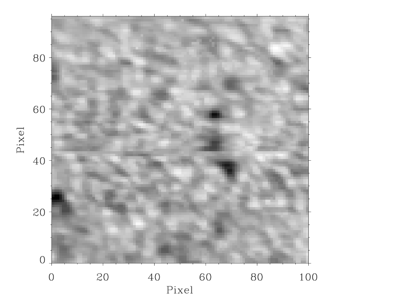
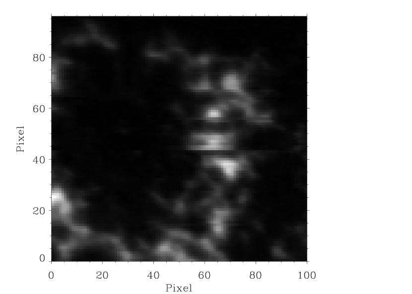
Figure 6: Map of the integrated absolute value of the circular polarization signal showing the annular active region with the internetwork region inside it.

We have performed exploratory spectropolarimetric observations of the spectral region around 15260 Å with the Tenerife Infrared Polarimeter (TIP; Martínez Pillet et al., 1999) mounted on the Vacuum Tower Telescope (VTT) at Izaña (Tenerife). The observations were taken during June 8^th 2002. We performed a scanning of a magnetically enhanced region of the quiet solar photosphere containing an enhanced network region of circular shape with an internetwork region inside. The seeing conditions were not especially good and the spatial resolution was of the order of $\sim$1.4”. The region was situated very close to the disk center ($\mu\approx 1$) and three small pores were also in the field of view. The left panel of Figure 6 shows an image taken in the local continuum of the 15262.702 Å line. The right panel of the figure shows the map of the integrated absolute value of the circular polarization signal. The annular enhanced network region is clearly seen in white. The polarimetric signals of the annular region are quite strong in the Mn I line. Except for very few points, the linear polarization signals could not be detected. However, we detected Stokes $V$ profiles produced by the longitudinal component of the magnetic field vector. Outside the annulus, the circular polarization signals were very weak.

The value of the signal-to-noise in the observed internetwork region is poor. In order to increase it, we have carried out a de-noising procedure based on the PCA decomposition of the Stokes $V$ data. After having obtained the eigenvectors along the directions of maximum covariance, the Stokes $V$ data has been projected on a manifold of reduced dimension using the first 8 eigenvectors (those that carry the statistically most relevant information). We have verified that this approach highly reduces the noise without introducing strong perturbations in the Stokes profiles with respect to the original ones.

4 Results and Discussion

4.1 Stokes $V$

Even after applying the above-mentioned noise reduction technique, the observations do not allow us to investigate in detail the Stokes $V$ profiles pixel by pixel. Therefore, we have focused on a statistical approach by means of a Stokes $V$ profile classification. In order to perform this classification, we have used a self-organizing map (SOM; Kohonen, 2001), also known as Kohonen’s network. The SOM is a special kind of neural network that is usually applied for visualization and classification purposes (e.g., Maehoenen & Hakala, 1995; Brett et al., 2004). It can be considered as a nonlinear mapping between the high-dimensional input space of Stokes parameters (in fact the space spanned by the first 8 eigenvectors of the PCA decomposition) and a regular two-dimensional grid. It consists of a two-dimensional grid of neurons where each neuron is associated with a feature in the original high-dimensional input space (the Stokes profiles observed for all the pixels in our field of view), with nearby neurons containing features that present similarities. In a way similar to a PCA classification, the SOM is an unsupervised classification method and it is capable of clustering data in the input space parameter. The PCA classification can only search for linear features in the high-dimensional input space. In this sense, the SOM classification produces much better results because it can detect nonlinearities in the input space. Since the classification is performed in an iterative scheme with initially random profiles in all the neurons, the final result typically depends on the number of neurons and on the initial configuration. This is produced by local minima in the learning process. Therefore, it is fundamental to carry out the learning process a sufficiently large number of times and verify that the same solution is obtained in a large fraction of such runs. A more detailed description is presented in Appendix A.

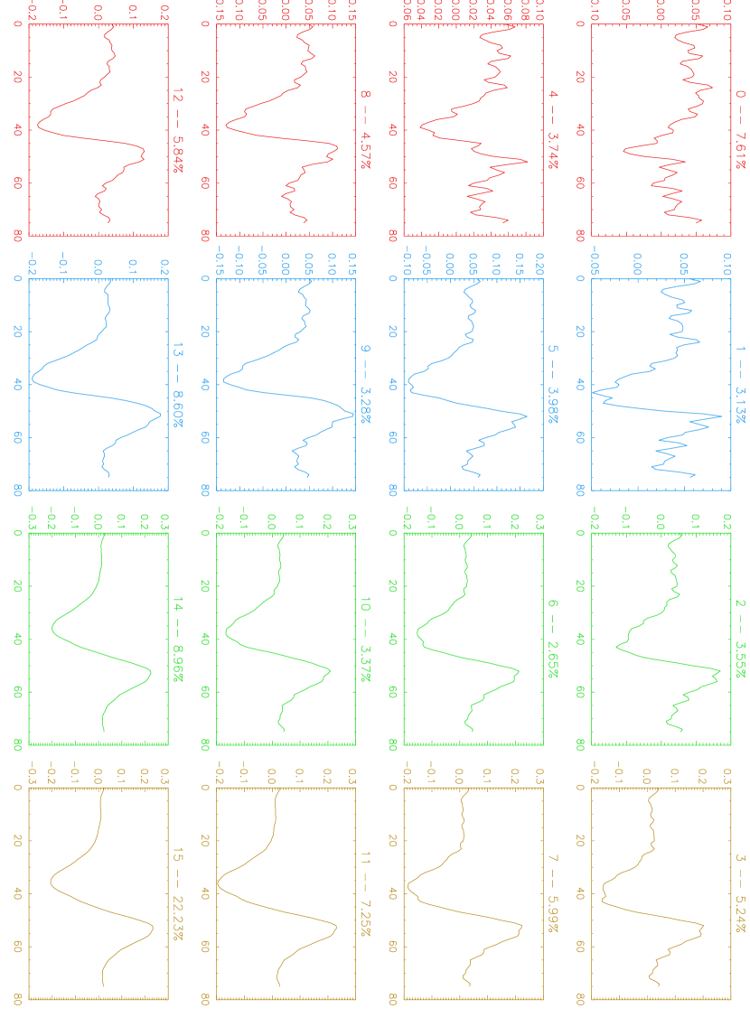
Figure 7: Classification obtained using a self-organizing map with a network of 4x4 neurons.

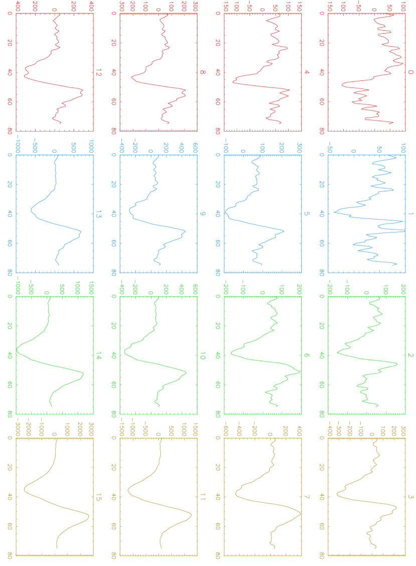
Figure 8: Average profile obtained from all the profiles belonging to each class in the 4x4 case.

The Stokes $V$ profiles are first normalized so that each profile has unit length if considered as a vector. We have carried out two different classifications, one with a 4$\times$4 map and another one with a 6$\times$6 map, obtaining quantitatively similar results. For clarity purposes, we only show the results of the 4$\times$4 map. The resulting profiles assigned to each neuron of the map are shown in Fig. 7. It presents profiles with the typical antisymmetric shape in one corner, while the profiles become more and more distorted when moving towards the opposite corner. The profile associated with each neuron that the SOM classification produces may not have physical sense. In order to overcome this problem, we have calculated the Stokes $V$ profile corresponding to each neuron by averaging all the pixels that have been associated with each class. The results are shown in Fig. 8.

It is immediate to verify that the SOM has generated a classification in which profiles are ordered according to the field strength (see Fig. 3). In each row, profiles associated with stronger fields (profiles in which the two peaks in the blue lobe are absent or hardly present) are located more to the right. The magnetic field decreases for the profiles located to the left because the two peaks in the blue lobe present a value of $r_{\mathrm{I}}$ that increases monotonically. One can argue that this may be produced by the presence of noise. As an argument in favor of the physical significance of the SOM classification, we can say that it has been carried out without any knowledge of the physical ingredients that produce these hyperfine signatures. As a result, since the final classification shows profiles that follow the trend obtained from the theory (Fig. 3), we are inclined to think that these features are real and not produced by noise. The ratio of the two peaks is smaller than 1 for large fields (above $\sim$900 G) and they become larger than 1 for weaker fields. Of course, such a one-to-one relation between peak ratio and magnetic field strength is only possible in the case that only one field strength is present within the resolution element. In the more general situation where a combination of magnetic fields is present in the resolution element, this association is not possible. In spite of this, the presence of the hyperfine signature in the blue lobe of the Stokes $V$ profiles indicates the presence of a field predominantly weaker than $\sim$700 G within the resolution element. In this sense, the 15262.702 Å line presents a diagnostic potential similar to that of the Mn I lines investigated by López Ariste et al. (2002, 2006). The profiles in the top left part of the map are associated with weak fields in which noise and the presence of mixed polarities plays an important role. For this reason, these profiles are highly distorted. For a fixed column in the SOM, the vertical variation of the profiles appears to be also related to the strength of the field, with the field decreasing when moving upwards in each column.

For comparison purposes, Fig. 7 indicates the percentage of points in the observed map that are associated with each neuron of the SOM. A large portion of the field-of-view is covered by the enhanced network region, so that the most abundant profiles are associated with those of stronger fields. In order to better understand the classification carried out by the SOM, we indicate the location of each class in the observed map in Fig. 9. The background images in the figures represent (in grayscale) the class of each point as obtained with the SOM. Each panel represents one of the rows of the classification network. Each color is associated with the profiles belonging to the columns of each row. The neurons of the fourth row of the map are clearly associated with the points belonging to the magnetically enhanced region that include the three pores. The neurons of the first row are clearly associated with the internetwork regions. The neurons belonging to the second and third row are associated with regions located between the network and the internetwork. The classification has detected the presence of ring-like regions that have been classified in the same row suggesting some kind of segregation of the magnetic field strength and a relation between the network and in the internetwork. Inside each ring-like structure, it is possible to find a distribution of magnetic fields whose distribution clearly shows smaller values for the inner parts than for the outer parts.

A magnetic field can be approximately associated with the profiles of the classes with the aid of the Milne-Eddington calculation and the calibration curve presented in Fig. 4. Obviously, this can only be done for those profiles that present the hyperfine signature in the blue lobe of the Stokes $V$ profile. The values used in this work are indicated in Table 1. The profiles for which the hyperfine features cannot be easily identified because the profile shows a clear antisymmetric shape are assigned an arbitrary field larger than 1 kG. We do not assign any magnetic field strength to the noisy profiles.

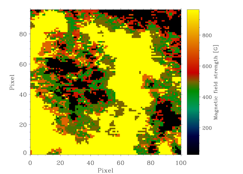
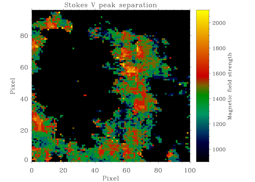
Figure 10: The left panel shows the magnetic field map obtained using the transformation between Stokes $V$ peak ratio and magnetic field obtained from the classification with the 4$\times$4 SOM. The values for the transformation are summarized in Table 1. The right panel shows the magnetic field strength obtained from the separation of the Stokes $V$ profile. We have only taken into account the profiles that present a clear antisymmetric shape.

Assuming only one magnetic component in the resolution element, it is possible to plot maps of the magnetic field strength. Figure 10 shows the map of field strength resulting from associating each class with a magnetic field strength. The kG fields have been saturated to 1000 G (they can be larger, but not smaller), while the noisy profiles are set to 0 G. It is interesting to note that the strong field strengths profiles are only placed in the magnetically enhanced region, specially in the pores and the surrounding regions. When we move towards the center of the internetwork region through the network-internetwork separation layer, the field strength rapidly decreases to the sub-kG regime.

Although the majority of the profiles coming from the network region have been classified as kG, it is possible to clearly identify the shape and position of the peaks of the Stokes $V$ profiles. Consequently, we have calculated the field strength associated with each profile measuring the wavelength separation between the peaks of the blue and red lobes and using the calibration curve presented in the right panel of Fig. 5. The results are shown in the right panel of Fig. 10. The strongest fields are associated with the pores, with field strengths above 1600 G and with 2000 G at some points. An estimation of the filling factor can be carried out assuming two components with the same thermodynamics, one magnetic and the other non-magnetic. The amplitude of the peak in the strong field regime arrives to 10 % for a filling factor of 1 (see Fig. 3). The amplitude of the strongest Stokes $V$ signals (those of the pores) is $\sim$3 %. This suggests that the maximum filling factor of the kG elements in the pores might be of the order of 30 %.

4.2 Stokes $I$

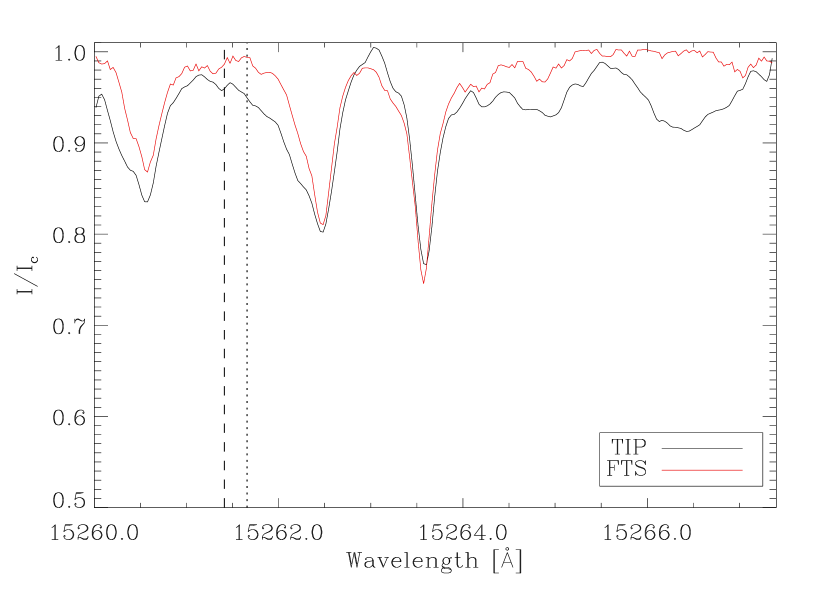
Figure 11: Intensity spectrum observed with TIP (black curve) and the one from the FTS atlas (red curve). We indicate with a vertical dotted line the wavelength where we take the continuum 1. This continuum forces the largest peak ratios of the Mn I line to be close to 2, the theoretical limit. The dashed line indicates the wavelength where we take the continuum 2, that can be considered as an upper limit.

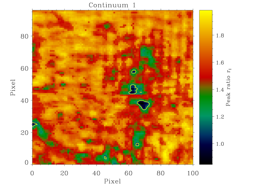
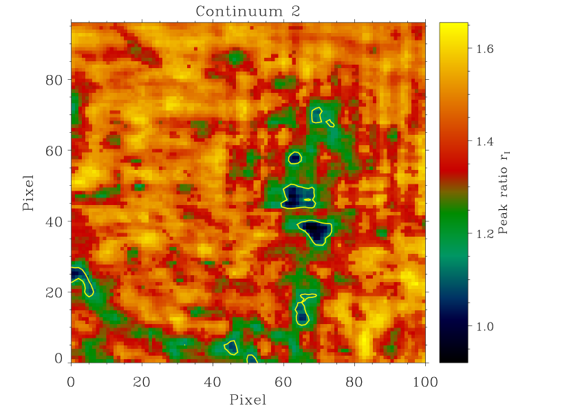
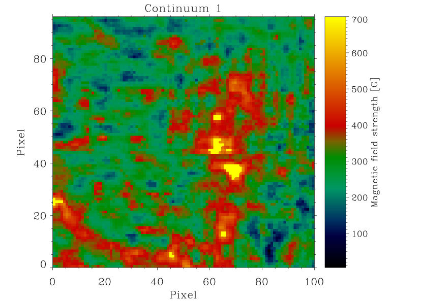
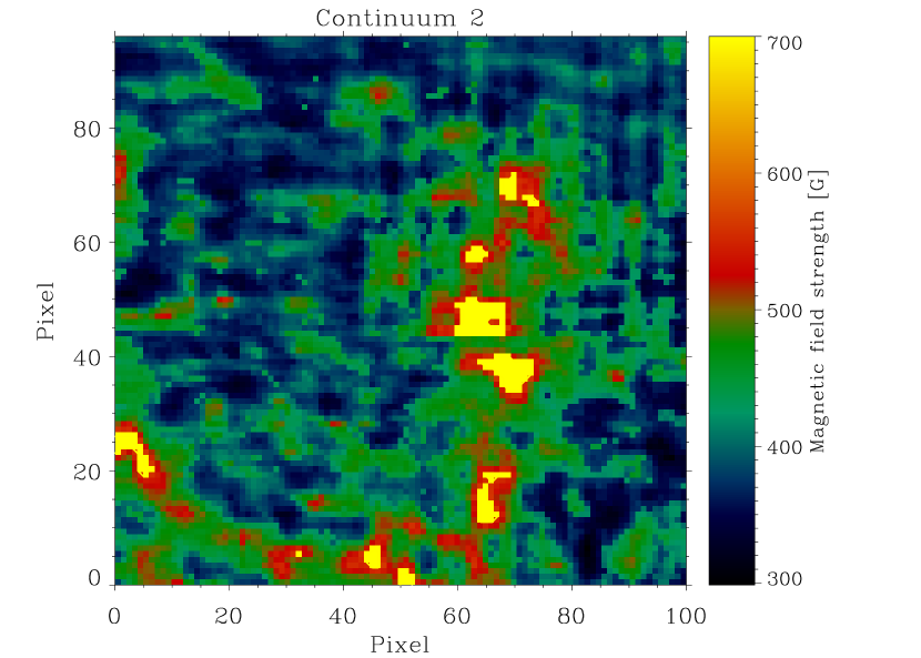
Figure 12: The upper panel shows the horizontal variation of the peak ratio measured in the intensity profile. The left panel is the ratio obtained using the continuum indicated in Fig. 11 with a dotted line, while the right panel is the ratio obtained using the continuum marked in Fig. 11 with a dashed line. We indicate the region where the ratio is smaller than 1.14, where two possible values of the magnetic field are associated with the same ratio. The lower panel indicates the value of the magnetic field obtained from the ratio using the calibration given by Fig. 4. The pixels where the ratio is smaller than 1.14 are indicated with a constant field of 700 G.

The presence of hyperfine structure allows us to use the intensity profile of the 15262.702 Å Mn I line as a powerful diagnostic tool. According to the Milne-Eddington results, the line presents two peaks whose ratio is close to 2 for zero magnetic field. This ratio can be easily measured in the observations. The most important source of problems is that the ratio critically depends on the exact value of the continuum. Figure 11 shows the comparison between one of the profile in the internetwork regions and the FTS atlas. The peak ratio given by the FTS atlas is $\sim$1.75, equivalent to a field of the order of $\sim$250 G using the calibration curve shown in Fig. 4. A comparison between the observed TIP spectrum and the FTS atlas indicates that the observed Stokes $I$ spectrum contains several spurious features. These features make it difficult to fix a value for the continuum. Following a conservative approach, we have selected two different values of the continuum. These values are indicated with vertical lines in the upper panel of Fig. 12. The two values of the continuum are chosen so that they represent an upper and lower limit of the continuum. The weaker continuum (vertical dotted line) is chosen so that the largest value of the ratio is smaller than 2. The reason is that ratios larger than 2 are not compatible with the results presented in Fig. 3. As a consequence, the magnetic field strengths obtained from these ratios represent a lower boundary for the true magnetic field strength distribution. The larger value of the continuum (vertical dashed line), chosen as an upper limit of the continuum, will give smaller ratios and, consequently, larger values of the magnetic field strength. This might be considered as an upper limit for the true magnetic field strength distribution.

The upper panel of Figure 12 shows the value of the ratio of the two peaks of the intensity profile for all the points in the field-of-view for the two values of the continuum. It is clearly seen that the smaller values of the ratios are correlated with the magnetically enhanced region, as expected from the previous considerations. Due to the presence of two solutions for peak ratios below $\sim$1.14, the points that fulfill this criterion are indicated in the map with contours. Fortunately, this criterion is only fulfilled in those regions of the map that coincide with the pores, where we expect the strongest fields. The smooth variation of the ratio between these strong field regions and the internetwork regions suggests a smooth variation in the distribution of fields. This smooth behavior also discards the noise as the responsible for the variations of the peak ratio.

Additionally, we have verified that the observed peak separation in Stokes $I$ is constant over the whole field-of-view, even for the enhanced network and the pores. The profiles of these points present peak ratios close to 1, which is indicative of moderately strong fields (of the order or above $\sim$500 G). However, since we do not detect any peak separation from the zero-field case ($\sim 0.23$ Å), we have to conclude that the average magnetic field that we are measuring with Stokes $I$ cannot be much stronger than $\sim$600 G.

We apply the calibration curve to transform the observed ratios into magnetic field strength. Since this measurement of the magnetic field strength has been carried out with Stokes $I$, it does not suffer from cancellation effects. Therefore, it represents an average value of unknown nature of the magnetic field per resolution element (see §4.6). The lower panels of Fig. 12 show the magnetic field strength maps. The maximum value of the magnetic field strength shown in the maps is 700 G. Stronger fields are represented with the same color coding. This maximum value are obtained at the points where the peak ratio is smaller than $\sim$1.14.

The previous analysis allows us to calculate some statistical properties of the magnetic field traced with the Stokes $I$ profiles. The left panels of Fig. 13 represent the histogram of the ratios obtained for the whole field-of-view using the two assumed values of the continuum. The behavior is very well represented by an exponential for ratios below $\sim$1.6. These histograms clearly show that the maximum ratio obtained for the smallest value of the continuum is 2, while the maximum value of the ratio turns out to be smaller when the second value of the continuum is chosen. We point out that almost all the points with ratios below 1.6 ($\sim$30% of the field of view) are located in the most active region. The points in the internetwork region have systematically ratios above 1.6.

In order to see this behavior in more detail, we have separated the points belonging to the network and those belonging to the internetwork. A pixel is assigned to the network when the maximum of the $V/I_{c}$ profile is above 1.6$\times$10^-3. We have verified that this value provides a good isolation of the network region. The histograms of the network points are shown in Figure 13 as dotted lines while the histograms of the internetwork points are shown as dashed lines. The histogram of the internetwork points peaks at $\sim$1.75 and it rapidly falls when moving towards higher ratios. The contribution of the internetwork to the points with ratios smaller than 1.6 is also small. The histogram of the internetwork region closely resembles a gaussian centered at a peak ratio of $\sim$1.75, equivalent to a gaussian centered at a magnetic field strength of $\sim$200 G. Concerning the network, the histogram has a less gaussian shape, with a peak at a ratio of $\sim$1.5, equivalent to a magnetic field strength of $\sim$350 G.

In an effort to understand the previous histograms, we have separated the internetwork histograms in granules and intergranules. Our observations were carried out with quite bad seeing conditions, so that the spatial resolution is about 1.4”. Consequently, the separation of the granular and intergranular regions is not very reliable. The granules are obtained as the set of points whose continuum intensity is larger than 1$\sigma$ above the mean continuum intensity of the whole internetwork. The intergranular regions are obtained as the set of pixels whose continuum is smaller than 1$\sigma$ below. The percentage of points assigned to granules is 15.8% while 15.3% of the points are classified as intergranules. The results are similar to those obtained by Socas-Navarro et al. (2004), who find 18% of granules and 17% of intergranules. The histograms of the peak ratios for these points are plotted in Fig. 14, indicating no apparent difference between granules and intergranules. Two possible explanations can be given. Firstly, the poor resolution produces a contamination between the light coming from the granular and the intergranular material, thus masking any possible intrinsic difference between them. Secondly, it is possible that there is no intrinsic difference and the background field that we measure with the Stokes $I$ profile is not spatially structured. The only way of investigating this in more detail is by performing observations with much better spatial resolution.

4.3 Incompatibility of Stokes $I$ and Stokes $V$ information

From the previous discussion, it is clear that the Stokes $V$ profiles that emerge from the network regions are associated with a quite strong field. We find profiles in the pores and nearby regions that we associate with fields above 1 kG due to the lack of hyperfine features in the blue lobe and that we confirm to be kG fields due to the peak separation in Stokes $V$. However, the ratio of Stokes $I$ peaks clearly indicates the presence of weak fields with an upper limit of $\sim$700 G. Furthermore, we do not detect enhanced Stokes $I$ peak separations in the pore with respect to what we see in the internetwork regions. An explanation might be the presence of relatively weak fields in the network (and in the pore) that have a large filling factor in comparison with the kG fields that are detected by the Stokes $V$ profile.

4.4 PDFs

Is it possible to retrieve the underlying probability distribution function of the magnetic field strength from the Stokes $I$ peak ratio measurements? Is the weak-field tail that is detected both in the internetwork and network histogram real? Does the measurement introduce any bias? In order to investigate these questions, a numerical experiment has been carried out. We have generated a set of $n=30000$ realizations of Stokes profiles with different values of a vertical magnetic field. The value of the magnetic field for each realization is selected following a given probability distribution function (PDF). Technically, the field strength for each one of the 30000 realizations is obtained by picking a random number $x$ following a uniform distribution in the interval $[0,1]$. By an appropriate variable transformation $y=f(x)$, the resulting numbers $y$ turn out to be distributed according to the desired distribution. Motivated by the results found in different works (Khomenko et al., 2003; Martínez González et al., 2006b), we have chosen to use exponential and maxwellian PDFs in this numerical experiment. A ME synthetic profile is obtained for each value of the field and the ratio between Stokes $I$ peaks is calculated. This procedure is also repeated by averaging the Stokes profiles emerging from $f$ consecutive realizations. Consequently, we end up with $30000/f$ average profiles for which the ratio is obtained. This mimics the loss of spatial resolution in the observation.

We synthesized 30000 Stokes profiles with a vertical field. The ¿ ¿ strength of the magnetic field strength is chosen to follow ¿ ¿ several probability distribution functions. In our case, we ¿ ¿ focus on an exponential and maxwellian PDFs. Technically, the ¿ ¿ field strength for each one of the 30000 realizations is obtained ¿ ¿ by picking a random number x following a uniform distribution in ¿ ¿ the interval [0,1]. By an appropriate transformation y=f(x), the ¿ ¿ resulting numbers y are distributed according to the desired ¿ ¿ distribution. For instance, for an exponential PDF, the number ¿ ¿ of synthetic Stokes profiles with weak fields is far larger than ¿ ¿ the number of Stokes profiles with strong fields. Summarizing, ¿ ¿ the 30000 realizations are in fact representative of the ¿ ¿ underlying PDF that we have assumed.

We will focus on the exponential PDFs of the form $P(B)\propto e^{-B/B_{0}}$. In such an exponential PDF, the probability of finding a point with a weak field is far larger than the probability of finding a strong fields. In the averaging process, the weak fields have more weight and the resulting Stokes $I$ profile presents systematically larger values of the ratio. As a consequence, the PDF retrieved from the ratio will have the fewer strong fields the larger the value of $f$. This is indeed observed in the experiment, as shown in the left panels of Fig. 15 for an exponential PDF with $B_{0}=200$ G and different values of $f$. With $f=1$, we are able to reproduce the slope of the original PDF and the exponential behavior for small fields. When $f$ increases, the strong field tail looses weight and moves towards weaker fields, increasing its slope. Thus, the slope of the recovered PDF combines information about the average field strength and the resolution.

A similar effect is also detected for the weak field tail, which moves towards higher fields when the spatial resolution gets worse. The explanation for this is the following. Only for extremely weak fields the peak ratio is close to 2. Larger fields always present smaller ratios. Therefore, after averaging several profiles, the ratio will always be smaller than 2 unless all the averaged pixels have $B=0$. A reduction of the number of profiles showing ratios close to 2 appears and the weak field tail moves towards stronger fields. This behavior dominates when $f$ increases because we average more points. It also dominates when $B_{0}$ increases because it reduces the amount of very weak fields in the averaging process.

The two processes together (reduction of the strong and weak field tails) tend to transform the retrieved PDF into a gaussian when the spatial resolution is not perfect. This behavior is also found in the experiment carried out with the maxwellian and seems to be a general property of the PDF when the resolution decreases. In the limit of a perfect resolution, it is possible to correctly recover the PDF. In the limit of an infinitely poor resolution, in which we only have one resolution element covering the whole observed area, the retrieved PDF is a Dirac delta function centered at the average field of the original PDF. In an intermediate regime, the retrieved PDF tends to a Gaussian that finally converges to a Dirac delta. Fortunately, the average field given by the distorted PDF is still the average field of the original PDF. This is a particularly important conclusion.

According to the previous calculations, the histograms presented in Fig. 13 indicate that the field distribution in the internetwork has a PDF whose average is in the range $200-350$ G for the two values of the continuum. The gaussian shape of the observed PDF suggests (at the light of the previous numerical experiments) that we are not resolving the fields. If we assume that the true PDF of the internetwork is an exponential, a direct comparison with the numerical experiment tends to suggest that $f=10$ is a plausible value for our observations. Striking is the fact that the inferred internetwork PDF is very similar to the one obtained in the numerical experiment for $B_{0}=200$ G and $f=10$. Not only the mean value of the field but the individual details of the recovered PDF are quite similar. If we assume that the field distribution does not change with height, the previous result implies that the horizontal scale at which the field is organized in the internetwork has to be of the order of $\sqrt{10}$ times smaller than our resolution element. For our resolution elements of the order of 1.4”-1.5”, this yields a value between 0.44”-0.48”.

Concerning the network field distribution, the peak gives an estimation of $B_{0}\sim 350$ G for the mean field strength. In the network, the shape of the PDF has a less gaussian shape than for the internetwork. The fields between 350 G and 550 G still present an exponential decay. This might imply that the scales of the magnetic field in the network are better resolved than in the internetwork. Note that the slope of the strong field tail of the network distribution is consistent with what is found in the numerical experiment using $f=10$ for an exponential PDF with $B_{0}=300-350$ G.

The previous numerical experiments have been also carried out with a maxwellian PDF. However, the observational results are not so favourably compared with the results obtained with such a maxwellian PDF. In this case, when the spatial resolution worsens, the field distribution converges to a gaussian centered at the mean field of the maxwellian given by $2B_{0}/\sqrt{\pi}$.

4.5 Agreement with other diagnostic tools

Are the previous results in agreement with those obtained by Trujillo Bueno et al. (2004, 2006) via analysis of the Hanle effect in Sr I and C₂? With the investigation of the Hanle effect in the 4607 Å line of Sr I, Trujillo Bueno et al. (2004) have concluded that, assuming an exponential PDF that does not distinguish between granules and intergranules, the best fit between the synthetic and observed linear polarization profiles is obtained for $\langle B\rangle\approx 130$ G. As it can be seen in Fig. 1 of Trujillo Bueno et al. (2004), this PDF with $\langle B\rangle\approx 130$ G gives a good fit to the inferred Hanle depolarization at $\mu=0.3$ (which corresponds to an atmospheric height of $\sim$300 km). However, in Fig. 1 of Trujillo Bueno et al. (2004) it can also be seen that for explaining the Sr I observations at $\mu=0.6$ (which corresponds to an atmospheric height of $\sim$200 km), the exponential PDF should have $\langle B\rangle\approx 200$ G. Our observations are close to disk center and, because the Mn I is weak, we expect it to be formed deeper than the Sr I line. Furthermore, the Sr I observations were performed in very quiet regions close to the North solar limb. Contrarily, our results are representative of an internetwork area that was encircled by an enhanced network region. Therefore, our results support those of Trujillo Bueno et al. (2004, 2006).

4.6 Flux cancellation

One of the most interesting diagnostic capabilities of this Mn I line is that Stokes $I$ and Stokes $V$ are sensitive to different aspects of the magnetic field distribution inside the resolution element. Stokes $I$ is sensitive to the total field distribution, and gives an idea of the total unsigned flux and the mean field strength in the resolution element. On the contrary, Stokes $V$ is sensitive to the part of the magnetic field distribution that is not cancelled out, that is, to the net flux. As a consequence, we can estimate the ratio between the net flux and the total flux, thus giving an idea of the amount of flux that cancels out. The net flux in the internetwork region has been obtained with the aid of the SOM classification. A net flux is assigned to each class of the SOM classification through the application of the weak-field approximation. We do not take into account those profiles marked as “noisy” in the SOM classification. Therefore, the flux cancellation $F_{\mathrm{net}}/F_{\mathrm{tot}}$ can be estimated directly. On the contrary, since the Stokes $V$ profiles in the network region are entering into the saturation regime, the amplitude of the $V$ profile is no longer proportional to the net flux. However, a rough estimation of the filling factor can be obtained by taking into account that the 15262.702 Å line is weak. In this case, the emergent Stokes parameters are proportional to the absorption coefficients, so that $(I_{\mathrm{c}}-I)\propto h_{I}$ and $V\propto fh_{V}$ (see, e.g., Landi Degl’Innocenti & Landolfi, 2004), with $I_{\mathrm{c}}$ being the continuum intensity. Making the additional assumption that the intensity profile is approximately equal to that obtained for the zero-field case (no enhanced peak separation is found even in the strong magnetized regions), we find that the emergent intensity at line center $I_{0}$ fulfills $(I_{\mathrm{c}}-I_{0})\propto H(0,a)/\sqrt{\pi}$. When Stokes $V$ is approximately described in the strong field regime, its value in one of the lobes can be written as $V_{0}\propto H(0,a)f\cos\theta/(2\sqrt{\pi})$. Finally, we obtain the following relation for the filling factor (Khomenko et al., 2003):

$$f\cos\theta\approx\frac{2V_{0}}{(I_{\mathrm{c}}-I_{0})},$$ (11)

where $\theta$ is the field inclination and $I_{0}$ is assumed to be not modified by the magnetic field. In spite of the strong simplifications assumed for the development of Eq. (11), we have verified via ME synthetic profiles that the previous approximate formula holds approximately for magnetic field strength values greater than $\sim$ 1 kG. From the previous estimation of the filling factor, it is possible to calculate the net magnetic flux $F_{\mathrm{net}}$ per resolution element as:

$$F_{\mathrm{net}}=f\cos\theta B_{\mathrm{V}}R^{2},$$ (12)

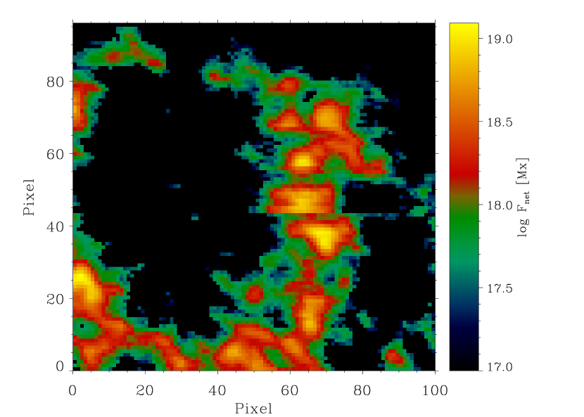
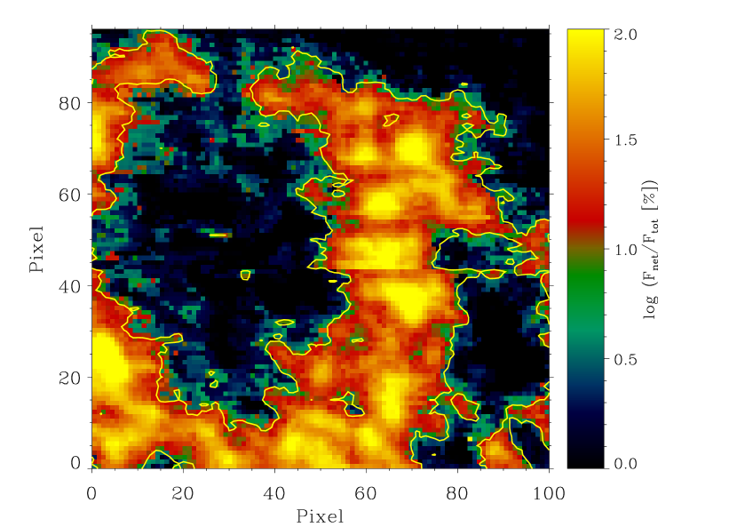
Figure 16: The left panel shows the flux in the network in a logarithmic scale. Note that the values of the flux are in accordance with the typical values. The right panel shows the ratio (in percentage) between the net flux and the total flux in the network and in the internetwork. A value of 2 (i.e., 100%) means that the no flux is cancelled, while a small value means that some flux is cancelled. The total flux is obtained from the field strength calculated from the Stokes $I$ peak ratio. The net flux has been obtained in two different ways. The points inside the contour, having Stokes $V$ profiles that clearly show clear indications of Zeeman saturation, we use Eq. (11). For the rest of points, we use a net flux associated with each class of the SOM classification using the weak-field approximation.

where $R^{2}$ is the area of the resolution element, in our case of the order of 1.4”$\times$1.4”. The magnetic field strength $B_{\mathrm{V}}$ has been obtained from the peak separation of the Stokes $V$ profile (represented in the the right panel of Fig. 10). The left panel of Fig. 16 presents the flux in logarithmic scale. The obtained values are in accordance with the typical values found in the network and in small pores (e.g., Zwaan, 1987). These results can be compared against those obtained from the peak ratio in Stokes $I$. Assuming that the value of the magnetic field obtained from the peak ratio (we call it $B_{\mathrm{I}}$) is representative of a volume filling field (with filling factor unity), the ratio

$$\frac{F_{\mathrm{net}}}{F_{\mathrm{tot}}}=\frac{2V_{0}}{(I_{\mathrm{c}}-I_{0})}\frac{B_{\mathrm{V}}}{B_{\mathrm{I}}}$$ (13)

gives us information about the cancellation of magnetic flux in those regions where Eq. (11) can be applied (i.e., the network, pores, etc.).

The ratio between the net and total fluxes is shown in the right panel of Fig. 16. The network presents ratios always above $\sim$10%. This indicates that the cancellation of flux in the network is always below 90%. The variation of the flux cancellation in the network is smooth. The pores present values of the ratios close to 100%, giving the indication that almost all the field in these strongly magnetized regions is in the form of a field with a well established direction. In these regions, the magnetic field strength diagnosed with Stokes $I$ and Stokes $V$ coincides. The cancellation ratio gets close to zero when moving towards the internetwork and it presents patches of equal value of the flux density (always below 10 Mx cm^-2). The contour shown in Fig. 16 indicates the separation between the points that belong to the network and those that belong to the internetwork. It is important to remind that, as already mentioned, the net flux in these regions has been obtained following a different approximation. However, it is interesting to point out that a smooth transition between the network and internetwork regions is found. The flux cancellation in the internetwork is such that the ratio between the net flux and the total flux is below 10% for more than 90% of the points.

In view of the approximations we have been forced to use due to the low Stokes $V$ signal of the Mn I line, it will be of great help to observe simultaneously this Mn I line together with other more magnetically sensitive lines so that the net flux can be estimated with more accuracy.

5 Conclusions

We have presented the results of a theoretical and observational investigation of a Mn I line located in the near-IR, which shows very attractive properties for magnetic field diagnostics. The combined effects of the larger Zeeman splitting present in the near-IR and the presence of strong perturbations on the Zeeman patterns due to the Paschen-Back effect, makes this line ideal for the diagnostic of magnetic fields in unresolved structures. The hyperfine structure produces modifications in the intensity profile of the line when a magnetic field is present, with a response that covers a large range of magnetic field strengths. The advantage over other Zeeman diagnostic tools is that it does not suffer from cancellation effects.

We have shown that the analysis of the ratio of the two peaks of the Stokes $I$ profiles measured in the quietest area of the observed field of view leads to a PDF of gaussian shape that is centered at 250-350 G, being unable to distinguish between granules and intergranules with our spatial resolution. This is a value that agrees with typical equipartition values in the photosphere and supports the Hanle-effect conclusion of Trujillo Bueno et al. (2004, 2006) that there is a substantial amount of hidden magnetic energy and unsigned flux in the quiet Sun. A theoretical investigation assuming different PDFs shows that the center of the inferred PDF gives information about the real PDF and that its gaussian shape is related to a degradation of the spatial resolution. Although higher signal-to-noise ratio observations are needed for obtaining better Stokes $V$ profiles, we have shown for the first time a map of how the flux cancels in unresolved magnetic elements.

In addition to the presence of pores and a magnetically active network, we must emphasize that the field of view of our observation contains an internetwork region where the net flux seldom amounts to 10% of the total flux. While the spatially average net flux found in very quiet internetwork regions (e.g., Khomenko et al., 2003; Martínez González et al., 2006b) is very close to zero (see, however, Domínguez Cerdeña et al., 2003, 2006a), we have a unipolar net flux in our internetwork region in accordance with the polarity of the surrounding network. The numerical experiments on turbulent dynamos and magnetoconvection carried out by Cattaneo and coworkers (Emonet & Cattaneo, 2001; Cattaneo et al., 2003; Cattaneo & Emonet, 2004) are initialized by a seed magnetic field that is then tangled up producing a mixed-polarity field with a distribution of field strengths such that the magnetic energy density is a significant fraction of the kinetic energy density. The field topology conserves any imbalance of net flux already present in the initial magnetic seed (Emonet & Cattaneo, 2001). In very quiet regions one can assume a random seed field resulting in a zero net magnetic flux. Our observations match, on the other hand, a scenario with an initial seed field with a non-zero net magnetic flux. Since the surrounding network of the observed field of view is magnetically enhanced and mostly unipolar, it is apparent that such a unipolar field may be ubiquitous through the encircled internetwork area and will play the role of a seed magnetic field with a non-zero net flux. Such a seed field might then be tangled up through dynamo action and/or magnetoconvection into the mixed-polarity fields that we find to constitute more than 90% of the total flux found in the observed internetwork region. The high level of mixing (90% at least) can be now qualitatively compared with simulations of magnetoconvection. Particularly instructive is Fig. 2 of Emonet & Cattaneo (2001) where their case 0 (whose seed field is a completely random field) results in a 100% cancellation, while their case 4 (with a seed field with a net flux equivalent to 200 G) results in a level of mixing smaller than 75%. The measured level of 90% would therefore translate into a seed field of a few G in apparent contradiction with the enhanced field found all around the internetwork area in our data. Such an apparent contradiction can be explained in two different ways. The first one is that the actual seed field through the internetwork is actually of just a few G and, therefore, results in a cancellation of 90% as predicted by simulations. The second possibility, and the one we prefer, is that solar magnetoconvection is more successful in mixing fields than present simulations, perhaps just because today’s numerical experiments are made with insuficient spatial resolution corresponding to relatively low Reynolds number as compared to the real values of the solar photosphere, at least in what concerns the magnetic description.

Another interesting conclusion is that the uncancelled flux reaches very high percentages (approaching 100%) in the pores and other magnetic concentrations over the network. In these regions Stokes V pointed toward kG fields, but Stokes I unveiled a greater contribution of weak fields under the 700 G threshold. Since both components appear to share the same polarity and there is not much cancellation, our analysis suggests that weak fields coexist with kG fields (carrying most part of the flux) even in these magnetically-enhanced regions.

The potential of this line has to be improved by simultaneously observing it with other lines, like the Fe I lines at 525 nm, 630 nm and 1.56 $\mu$m and the Mn I line at 5537 Å. Furthermore, other lines with hyperfine structure can be found in the red and near-IR that can be of great diagnostic potential if they can be observed simultaneously.

Finally, this IR Mn I line may be of great interest for diagnosing magnetic fields in other stars apart from the Sun. The line ratio we have developed can be obtained provided one observes with sufficiently high spectral resolution observation and for sufficiently slow rotators. With our line ratio technique, it should be possible to estimate the average magnetic field strength of the star.

Appendix A Self-organizing maps

Self-organizing maps (SOM) are one of the multiple variants of artificial neural networks. They are trained using unsupervised learning techniques and they produce a low-dimensional representation of the training sample. One of the most important characteristics is that the low-dimensional representation tries to preserve the topological properties of the input space (training samples), so that nearby samples are mapped into nearby neurons (Kohonen, 2001). They have been mostly applied to the visualization of high-dimensional data.

The self-organizing map consists on a single layer feedforward neural network. The output layer is arranged in a low-dimensional (usually 2D or 3D) grid of $N_{\mathrm{out}}\times N_{\mathrm{out}}$ neurons. The input layer is formed by a set of $N_{\mathrm{in}}$ neurons, where $N_{\mathrm{in}}$ is the dimensionality of the input training space. The network is fully connected, in the sense that every neuron of the output layer is connected to every neuron of the input layer. Each neuron of the output layer is associated with a weight vector $\mathbf{W}\in\mathbb{R}^{N_{\mathrm{in}}}$, i.e., with the dimensionality of the input space.

Motivated by how sensory information is handled in different parts of the brain, the goal of the unsupervised learning algorithm is to associate different parts of the map to different parts of the input space. Therefore, similar parts of the map will produce larger response when several input data that share a given property is shown to the neural network.

The iterative scheme is started by initializing the weights with small random numbers (it is also possible to initialize by uniformly sampling the subspace generated by the first two largest principal components of the input space). The iteration number is accounted for by the discrete index $t$. Each iteration needs to repeat the following update rule for each input data (Kohonen, 2001):

$$\mathbf{W}_{i}(t+1)=\mathbf{W}_{i}(t)+h_{i}(t)\Big{[}\mathbf{X}(t)-\mathbf{W}_{i}(t)\Big{]},$$ (A1)

where $\mathbf{W}_{i}(t+1)$ is the weight associated with each neuron $i$ at iteration $t+1$, $\mathbf{X}(t)$ represents the input vector, while $\mathbf{h}_{i}(t)$ is the so-called neighborhood function. The neighborhood function is built in the following way. First of all, the euclidean distances between all the neuron’s weights and the input vector are calculated. The neuron with the smallest distance is known as the best-matching node, whose distance with the input vector is $r_{c}$. The neighborhood function is used for propagating the information of the input vector to the surrounding neurons, and it is usually written as:

$$h_{i}(t)=\alpha(t)\exp\Bigg{(}-\frac{\parallel r_{c}-r_{i}\parallel^{2}}{2\sigma^{2}(t)}\Bigg{)},$$ (A2)

where $r_{i}$ is the euclidean distance between the weight of neuron $i$ an the input vector. The functions $\alpha(t)$ (learning rate) and $\sigma(t)$ (width of the kernel) are some monotonically decreasing function of the index $t$ that control the spread of the neighborhood kernel. For the initial iterations, the large width of the kernel leads to a convergence in the global scale. When the width of the kernel is reduced, the convergence tends to be more local.

After a large number of iterations, convergence of the map is obtained. The weights of the neurons tend to be associated with patterns in the input data, with similar patterns being located in nearby neurons. Finally, it is possible to use the map to classify any input vector, whether it was in the learning set or not. The euclidean distance is calculated between the input vector and all the neuron’s weights. The neuron whose weight lies closest to the input vector will give the location in the map of the group in which the input vector has been classified.

Table 1: Peak ratio for each profile in the 4$\times$4 SOM.

Noisy	Noisy	Noisy	0.791
profile	profile	profile	(457 G)
0.9895	1.0425	1.129	1.219
(592 G)	(623 G)	(671 G)	(717 G)
0.747	0.757	$>$1kG	$>$1kG
(421 G)	(429 G)
0.814	0.843	$>$1 kG	$>$1 kG
(474 G)	(496 G)

Figure 1: Splitting (in cm^-1 of the upper and lower levels of the Mn I transition at 15262.702 Å. When the hyperfine structure is taken into account, both fine structure levels have six $F$ levels. Note that level crossings are present at fields as low as 200 G, thus leading to strong perturbations in the Zeeman patterns due to the incomplete Paschen-Back effect.

Figure 2: Zeeman pattern of the 15262.702 Å transition of Mn I for two different values of the magnetic field strength. The $\Delta M_{F}=-1$ components are in the upper panel pointing upwards, the $\Delta M_{F}=+1$ components are in the upper panel pointing downwards and the $\Delta M_{F}=0$ components are in the lower panel. The zero-field case shows only the allowed transitions between the $F$ levels of the upper and lower fine structure level. When the field increases, the degeneracy of the magnetic sublevels is broken and a large amount of components appear. The number of components is 171 for the $\Delta M_{F}=\pm 1$ transitions and 176 for the $\Delta M_{F}=0$ transitions.

Figure 3: Milne-Eddington synthetic profiles obtained for 100, 600, 900 and 1300 G. The thermodynamical parameters that have been employed ($v_{\mathrm{th}}=0.1$ Å, $\beta=1$, $\eta_{0}=2$) approximately fit the observed Stokes $I$ profiles in the internetwork regions. Focusing on Stokes $V$, the presence of a blue peak weaker than a red peak (both in the blue lobe of the Stokes $V$ profile) indicates fields below $\sim$700 G. Furthermore, the detection of peaks in the blue lobe indicates the presence of fields below $\sim$1000 G.

Figure 4: Ratio of the peaks produced by the hyperfine structure in the Stokes $V$ profile (left panel) and in the Stokes $I$ profile (right panel). The ratio of the peaks in Stokes $V$ cannot be correctly defined for fields above 1000 G because the hyperfine features disappear. Nevertheless, their presence in an observed Stokes $V$ profile is indicative of fields well below 1000 G. The ratio of the peaks in Stokes $I$ has a unicity problem for fields above $\sim$600 G, although one of the two possible solution can be chosen in terms of the peak separation shown in Fig. 5.

Figure 5: Separation of the peaks in the Stokes $I$ profile (left panel) and in the Stokes $V$ profile (right panel). The peak separation for Stokes $I$ remains constant for fields below $\sim$600 G and increases linearly for stronger fields. For Stokes $V$, the peak separation (defined only above $\sim$900 G) increases also linearly in the strong field regime.

Figure 9: Location of the profiles belonging to each class in the 4x4 classification.

Figure 13: Histograms of the peak ratio (left panels) and magnetic field strength using the calibration presented in the paper (right panels). We present the results obtained for the two selected values of the continuum. We also include the histogram of the points that belong to the internetwork.

Figure 14: Histograms of peak ratios for the granular and intergranular pixels separately. Both panels have been calculated with different values of the continuum. Note that the histograms are similar, giving an indication that we are not able to distinguish between granules and intergranules.

Figure 15: Histogram of the magnetic field recovered by using the peak ratio of Stokes $I$ in the numerical experiment. The original PDFs are exponentials with $B_{0}=200$ G and $B_{0}=350$ G (shown in all the panels with dashed lines) and is representative of the internetwork and network results, respectively. The solid line represents the recovered PDF using different values of $f$ that reproduces the loss of spatial resolution. Note that the slope and the behavior for weak fields is correctly recovered when all the points are taken into account. When the resolution gets worse, the retrieved PDF tends to a Gaussian centered at $B_{0}=200$ G for the first case and $B_{0}=350$ G for the second case.

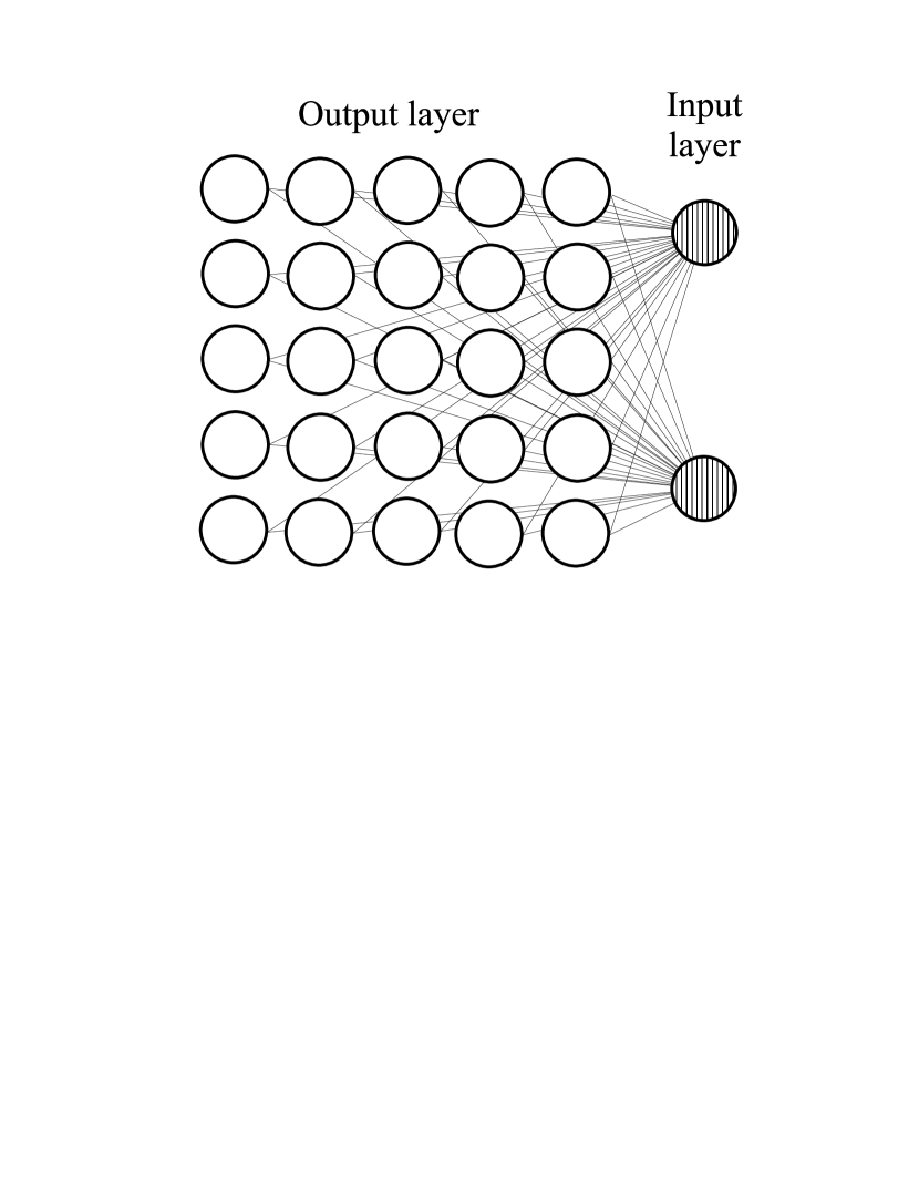
Figure 17: Topology of the self-organizing map. The input layer has dimension $N_{\mathrm{in}}$ and the output layer consists on a $N_{\mathrm{out}}\times N_{\mathrm{out}}$ map of neurons. A weight vector of dimension $N_{\mathrm{in}}$ is associated with each neuron.

References

- Brett et al. (2004) Brett, D. R., West, R. G., & Wheatley, P. J. 2004, MNRAS, 353, 369
- Casimir (1963) Casimir, H. B. G. 1963, On the Interaction Between Atomic Nuclei and Electrons (San Francisco: Freeman)
- Cattaneo (1999) Cattaneo, F. 1999, ApJ, 515, L39
- Cattaneo & Emonet (2004) Cattaneo, F., & Emonet, T. 2004, in 35th COSPAR Scientific Assembly, 4443
- Cattaneo et al. (2003) Cattaneo, F., Emonet, T., & Weiss, N. 2003, ApJ, 588, 1183
- Domínguez Cerdeña et al. (2003) Domínguez Cerdeña, I., Sánchez Almeida, J., & Kneer, F. 2003, A&A, 407, 741
- Domínguez Cerdeña et al. (2006a) —. 2006a, ApJ, 646, 1421
- Domínguez Cerdeña et al. (2006b) —. 2006b, ApJ, 636, 496
- Emonet & Cattaneo (2001) Emonet, T., & Cattaneo, F. 2001, ApJ, 560, L197
- Khomenko et al. (2003) Khomenko, E. V., Collados, M., Solanki, S. K., Lagg, A., & Trujillo Bueno, J. 2003, A&A, 408, 1115
- Kohonen (2001) Kohonen, T. 2001, Self-organizing maps (Berlin: Springer)
- Kurucz (1993a) Kurucz, R. 1993a, Phys. Scr., 47, 110
- Kurucz (1993b) —. 1993b, Atomic data for opacity calculations (Kurucz CD-ROM No.1)
- Landi Degl’Innocenti & Landolfi (2004) Landi Degl’Innocenti, E., & Landolfi, M. 2004, Polarization in Spectral Lines (Kluwer Academic Publishers)
- Lefèbvre et al. (2003) Lefèbvre, P.-H., Garnir, H.-P., & Biémont, E. 2003, A&A, 404, 1153
- Lin (1995) Lin, H. 1995, ApJ, 446, 421
- Lin & Rimmele (1999) Lin, H., & Rimmele, T. 1999, ApJ, 514, 448
- Lites & Socas-Navarro (2004) Lites, B. W., & Socas-Navarro, H. 2004, ApJ, 613, L600
- López Ariste et al. (2002) López Ariste, A., Tomczyk, S., & Casini, R. 2002, ApJ, 580, 519
- López Ariste et al. (2006) —. 2006, A&A, 454, 663
- Maehoenen & Hakala (1995) Maehoenen, P. H., & Hakala, P. J. 1995, ApJ, 452, L77
- Martínez González et al. (2006a) Martínez González, M. J., Collados, M., & Ruiz Cobo, B. 2006a, A&A, 456, 1159
- Martínez González et al. (2006b) Martínez González, M. J., Collados, M., & Ruiz Cobo, B. 2006b, in Solar Polarization 4, ed. R. Casini & B. W. Lites, ASP Conf. Ser., in press
- Martínez Pillet et al. (1999) Martínez Pillet, V., Collados, M., Bellot Rubio, L. R., Rodríguez Hidalgo, I., Ruiz Cobo, B., & Soltau, D. 1999, in Astronomische Gesselschaft Meeting Abstracts, vol. 15
- Press et al. (1986) Press, W. H., Teukolsky, S. A., Vetterling, W. T., & Flannery, B. P. 1986, Numerical Recipes (Cambridge: Cambridge University Press)
- Priest (2006) Priest, E. 2006, in The Many Scales of the Universe, ed. J. C. del Toro Iniesta
- Sánchez Almeida (2004) Sánchez Almeida, J. 2004, in ASP Conf. Ser. 325: The Solar-B Mission and the Forefront of Solar Physics, ed. T. Sakurai & T. Sekii, 115
- Sánchez Almeida et al. (2003) Sánchez Almeida, J., Emonet, T., & Cattaneo, F. 2003, ApJ, 585, 536
- Schrijver (2005) Schrijver, C. J. 2005, in ESA SP-596: Chromospheric and Coronal Magnetic Fields, ed. D. E. Innes, A. Lagg, & S. A. Solanki
- Semel (1981) Semel, M. 1981, A&A, 97, 75
- Socas-Navarro et al. (2004) Socas-Navarro, H., Martínez Pillet, V., & Lites, B. W. 2004, ApJ, 611, 1139
- Socas-Navarro & Sánchez Almeida (2002) Socas-Navarro, H., & Sánchez Almeida, J. 2002, ApJ, 565, 1323
- Stein & Nordlund (2003) Stein, R. F., & Nordlund, A. 2003, in Stellar Atmosphere Modeling, ed. I. Hubeny, D. Mihalas, & K. Werner, ASP Conf. Ser. 288 (San Francisco: ASP), 519
- Stenflo (1994) Stenflo, J. O. 1994, Solar Magnetic Fields. Polarized Radiation Diagnostics (Dordrecht: Kluwer Academic Publishers)
- Stenflo & Lindegren (1977) Stenflo, J. O., & Lindegren, L. 1977, A&A, 59, 367
- Trujillo Bueno (2001) Trujillo Bueno, J. 2001, in ASP Conf. Ser. 236: Advanced Solar Polarimetry – Theory, Observation, and Instrumentation, ed. M. Sigwarth, 161
- Trujillo Bueno (2005) Trujillo Bueno, J. 2005, in ESA SP-600: The Dynamic Sun: Challenges for Theory and Observations, ed. D. Danesy, S. Poedts, A. De Groof, & J. Andries, 7
- Trujillo Bueno et al. (2006) Trujillo Bueno, J., Asensio Ramos, A., & Shchukina, N. 2006, in Solar Polarization 4, ed. R. Casini & B. W. Lites, ASP Conf. Ser., in press
- Trujillo Bueno et al. (2004) Trujillo Bueno, J., Shchukina, N., & Asensio Ramos, A. 2004, Nature, 430, 326
- Vögler (2003) Vögler, A. 2003, PhD thesis, Göttingen University
- Zwaan (1987) Zwaan, C. 1987, ARA&A, 25, 83