The XMM–Newton wide-field survey in the COSMOS field. III:
optical identification and multiwavelength properties of a large sample of X–ray selected sources

Abstract

We present the optical identification of a sample of 695 X-ray sources detected in the first 1.3 deg² of the XMM-COSMOS survey, down to a 0.5-2 keV (2-10 keV) limiting flux of $\sim 10^{-15}$ erg cm^-2 s^-1 ($\sim 5\times 10^{-15}$ erg cm^-2 s^-1). In order to identify the correct optical counterparts and to assess the statistical significance of the X-ray to optical associations we have used the “likelihood ratio technique”. Here we present the identification method and its application to the CFHT I-band and photometric catalogs. We were able to associate a candidate optical counterpart to $\sim$90% (626) of the X-ray sources, while for the remaining $\sim$10% of the sources we were not able to provide a unique optical association due to the faintness of the possible optical counterparts (I${}_{\rm AB}>$25) or to the presence of multiple optical sources, with similar likelihoods of being the correct identification, within the XMM–Newton error circles. We also cross-correlated the candidate optical counterparts with the Subaru multicolor and ACS catalogs and with the Magellan/IMACS, zCOSMOS and literature spectroscopic data; the spectroscopic sample comprises 248 objects ($\sim$40% of the full sample). Our analysis of this statistically meaningful sample of X–ray sources reveals that for $\sim$80% of the counterparts there is a very good agreement between the spectroscopic classification, the morphological parameters as derived from ACS data, and the optical to near infrared colors: the large majority of spectroscopically identified broad line AGN (BL AGN) have a point-like morphology on ACS data, blue optical colors in color-color diagrams, and an X–ray to optical flux ratio typical of optically selected quasars. Conversely, sources classified as narrow line AGN or normal galaxies are on average associated with extended optical sources, have significantly redder optical to near infrared colors and span a larger range of X–ray to optical flux ratios. However, about 20% of the sources show an apparent mismatch between the morphological and spectroscopic classifications. All the “extended” BL AGN lie at redshift $<$1.5, while the redshift distribution of the full BL AGN population peaks at z$\sim$1.5. The most likely explanation is that in these objects the nuclear emission is not dominant with respect to the host galaxy emission in the observed ACS band. Our analysis also suggests that the Type 2/Type 1 ratio decreases towards high luminosities, in qualitative agreement with the results from X–ray spectral analysis and the most recent modeling of the X–ray luminosity function evolution.

1. Introduction

The primary goals of the “Cosmic Evolution Survey” (COSMOS, Scoville et al. 2007a) is to trace star formation and nuclear activity along with the mass assembly history of galaxies as a function of redshift and environment. Although there were early theoretical suggestions (e.g. Silk & Rees 1998), it was the tight relation observed in local galaxies between the black holes mass and the velocity dispersion (the M_BH-$\sigma$ relation, see e.g. Ferrarese & Merritt 2000; Gebhardt et al. 2000) and the fact that the locally inferred black hole mass density appears to be broadly consistent with the estimates of the mass accreted during the quasar phase (Fabian & Iwasawa, 1999; Yu & Tremaine, 2002; Elvis, Risaliti, & Zamorani, 2002; Marconi et al., 2004; Merloni, 2004) that made it clear that BH–driven nuclear activity and the assembly of bulge masses are closely linked. This realization has led to a large number of theoretical studies, suggesting feedback mechanisms to explain this fundamental link between the assembly of black holes (BH) and the formation of spheroids in galaxy halos (Di Matteo et al. 2005; Menci et al. 2004 and reference therein).

In this framework, the hard X–ray band is by far the cleanest one for studying the history of accretion onto black holes in the Universe, being the only band in which emission from accretion processes clearly dominates the cosmic background. The detailed study of the nature of the hard X–ray source population is being pursued by complementing deep pencil beam observations with shallower, larger area surveys (see Brandt & Hasinger 2005 for a recent review). Indeed, in the recent years, large efforts have been dedicated to the optical to radio characterization of X–ray sources selected at different X–ray depths (see, among the most recent: the XBoötes survey (Brand et al., 2006), the Serendipitous Extragalactic X–ray Source Identification SEXSI (Eckart et al., 2006), the Extended Groth strip EGS (Georgakakis et al., 2006), the HELLAS2XMM survey (Cocchia et al., 2007)). In particular, sizable samples of objects detected at the bright X–ray fluxes ($\gtrsim 10^{-14}$ erg cm^-2 s^-1) over an area of the order of a few square degrees are needed to cover the high luminosity part of the Hubble diagram and to obtain, together with samples from narrower and deeper pencil–beam observations, a well constrained luminosity function with a similar number of sources per luminosity decade and redshift bin. The results from both deep (Alexander et al., 2003; Barger et al., 2003; Giacconi et al., 2002; Szokoly et al., 2004; Hasinger et al., 2001) and shallow surveys (Fiore et al., 2003; Green et al., 2004; Steffen et al., 2004) have unambiguously unveiled a differential evolution for the low– and high–luminosity AGN population (Ueda et al., 2003; Barger et al., 2005; Silverman et al., 2005; Hasinger, Miyaji & Schmidt, 2005; La Franca et al., 2005). However, in these studies, the evolution of the high-luminosity tail of the obscured AGN luminosity function remains a key parameter still to be determined. The best strategy to address this issue is to increase the area covered in the hard X–ray band, and the corresponding optical-NIR photometric and spectroscopic follow-up, down to F${}_{2-10keV}\sim 5\times 10^{-15}$ erg cm^-2 s^-1, where the bulk of the XRB is produced.
Another important issue in AGN studies is the determination of the global Spectral Energy Distributions (SEDs), over the widest possible frequency range, of different types of AGN. Large samples of AGN have been assembled using different selection criteria at different frequencies (e.g. radio, infrared, optical-UV, X-ray); however, the lack of complete multi-wavelength coverage for many of these samples makes it difficult the comparison of the properties of different classes of AGN. For example, while the average SED of optically and radio selected bright quasars has been reasonably well known for more than a decade (Elvis et al., 1994), little is still known about the SEDs of lower luminosity X-ray selected AGNs and, in particular, of the obscured ones. This reflects into a significant uncertainty in the estimate of the bolometric correction ($k_{bol}$, i.e. the correction from the X–ray to the bolometric luminosity) to be applied to the observed luminosity of X-ray selected AGN and, in turn, on the estimates of the Eddington luminosities and of the masses of the central black holes (Fabian, 2004). Recent results on high–redshift quasars have shown that the overall X–ray to optical spectral slope ($\alpha_{\rm ox}$, usually measured between 2500 Å and 2 keV, e.g. Tananbaum et al. 1979) and the corresponding $k_{bol}$, is a function of the AGN luminosity, with the low luminosity objects having a lower $k_{bol}$ (Vignali, Brandt & Schneider, 2003; Fabian, 2004; Steffen et al., 2006). It is therefore clear that, in order to get a complete census of the luminosity output of AGN, a multi-wavelength project is needed: only in this way can the SEDs from radio to X-rays of a large sample of AGN, selected at different frequencies, be compiled.

The XMM–Newton wide-field survey in the COSMOS field (hereinafter: XMM-COSMOS) is an important step forward in addressing the topics described above. The $\sim 2$ deg² area of the HST/ACS COSMOS Treasury program (Scoville et al., 2007b), bounded by $9^{\rm h}57.5^{\rm m}<$R.A.$<10^{\rm h}03.5^{\rm m}$; $1^{\rm d}27.5^{\rm m}<$DEC$<2^{\rm d}57.5^{\rm m}$, has been surveyed with XMM–Newton for a total of $\sim$800 ks during AO3, and additional 600 ks have been already granted in AO4 to this project. When completed, XMM-COSMOS will provide an unprecedently large sample of X-ray sources ($\mathrel{\hbox to0.0pt{\lower 3.0pt\hbox{$\mathchar 536\relax$}\hss}\raise 2.0pt\hbox{$\mathchar 318\relax$}}2000$), detected on a large, contiguous area, with complete ultraviolet to mid-infrared (including Spitzer data) and radio coverage, and almost complete spectroscopic follow–up granted through the zCOSMOS (Lilly et al., 2007) and Magellan/IMACS (Impey et al., 2007) projects.
The XMM-COSMOS project is described in Hasinger et al. (2007). The X–ray point source counts from the first 800 ks of the XMM–Newton observations obtained so far are presented in Cappelluti et al. (2007), while the properties of extended and diffuse sources are described in Finoguenov et al. (2007). First results from the spectral analysis of AGN with known redshift and high counting statistics are presented in Mainieri et al. (2007).
This paper presents the optical identification of X–ray point sources detected in this first year of the XMM–Newton data, and the first results on the multiwavelength properties of this large sample of X-ray selected AGN.
The paper is organized as follows: Section 2 presents the multiwavelength datasets and describes the method used to identify the X-ray sources and its statistical reliability; the X–ray to optical and near infrared properties are presented in Sect. 3, along with preliminary results from the ongoing spectroscopic follow–up; in Sections 4 and 5 we discuss and summarize the most important results. Throughout the paper, we adopt the cosmological parameters $H_{0}=70$ km s^-1 Mpc^-1, $\Omega_{m}$=0.3 and $\Omega_{\Lambda}$=0.7 (Spergel et al., 2003).

Figure 1.— Observed magnitude distribution of all the optical objects detected in the $I$ band within a radius of 3″ around each of the 674 point-like X–ray sources fainter than I_AB=16 (solid histogram), together with the expected distribution of background objects in the same area (n(m), dashed histogram). The difference between these two distributions (dotted histogram) is the expected magnitude distribution of the optical counterparts. The smooth curve fitted to this histogram (dotted line) has been used as input in the likelihood calculation (q(m)).

2. X-ray source identification

2.1. Optical and X–ray datasets

The XMM-COSMOS X-ray source catalog comprises 1390 different point–like X–ray sources detected over an area of $\sim$2 deg² in the first-year XMM–Newton observations of the COSMOS field (Hasinger et al., 2007; Cappelluti et al., 2007). In this paper, we limit our analysis to the sources detected in the first 12 XMM-COSMOS observations (over a total of $\sim$1.3 deg²), for which both the X-ray source list and the optical catalogs were in place in June 2005, and a substantial spectroscopic follow-up already exists. These fields are flagged in Table 1 in Hasinger et al. (2007), and the average exposure time is of $\sim 25ks$ ($\sim 40$ ks in the overlapping region, see Hasinger et al. 2007 for more details). The catalog paper with the identification from the entire XMM-COSMOS survey is in preparation and will rely strongly on the identification procedure described here.
The 12 fields X-ray catalog (hereinafter: 12F catalog) comprises 715 X-ray sources detected over a total of $\sim$1.3 deg². From the 12F catalog we removed 20 sources classified as extended by the detection algorithm (see Cappelluti et al. 2007 for a description of the adopted detection algorithm). The observed X–ray emission from most of these sources is likely to be due either to groups/clusters of galaxies, or to the contribution of two or more X–ray sources close to each other. In both cases, an association with a unique optical counterpart is not possible. The total number of point-like X-ray sources in the 12F catalog, detected in at least one of the X-ray bands is therefore 695. Of these, 656 are detected in the soft band (0.5-2 keV), 312 in the medium band (2-4.5 keV; 38 only in the medium band), and 47 in the hard band (4.5-10 keV; 1 only in the hard). The X–ray centroids of these 695 point-like X-ray sources have been astrometrically calibrated using the SAS task eposcorr, as described in Cappelluti et al. (2007); the resulting shift of $\sim$1^′′ ($\Delta$($\alpha$)=0.99^′′; $\Delta$($\delta$)=0^′′) was applied to all source positions.
As a first step in the identification process, we used the I–band CFHT/Megacam catalog (Mc Cracken et al., 2007), which, although slightly shallower than other available data (e.g. the Subaru B,g,V,R,I and z photometric data, see Capak et al. 2007), has the advantage of having reliable photometry even at bright magnitudes (I${}_{\rm AB}\mathrel{\hbox to0.0pt{\lower 3.0pt\hbox{$\mathchar 536\relax$}\hss}\raise 2.0pt\hbox{$\mathchar 316\relax$}}19$), where the Subaru photometry starts to be significantly affected by uncertainties due to saturation.
At magnitudes brighter than I${}_{\rm AB}=16$, only $\sim$0.24 sources are expected by chance in a 3^′′ error-circle around all the 695 X-ray sources on the basis of the background counts of the Megacam catalog; therefore we considered as secure optical identifications all the 21 sources brighter than I_AB=16 in the CFHT catalog and within 3^′′ from the X–ray centroids. For all the remaining X–ray sources (674) we used the method described in Sect. 2.2.
Then, we have cross-correlated the optical counterparts with the multicolor photo-z catalog (June 22th 2005 release, Capak et al. 2007). All the magnitudes are in the AB system (Oke, 1971), if not otherwise stated.

2.2. The method

Typical error-circles of XMM–Newton data ($\sim 5^{\prime\prime}$ arcsec radius at 95% confidence level) often contain more than one source in deep optical images, so that the identification process is not always straightforward. Obviously, this is particularly true when the candidate counterparts are faint. We therefore decided to use the “likelihood ratio” ($LR$) technique, in order to properly identify the optical counterparts (Sutherland & Saunders, 1992; Ciliegi et al., 2003; Brusa et al., 2005). The $LR$ is defined as the ratio between the probability that the source is the correct identification and the corresponding probability of being a background, unrelated object (Sutherland & Saunders, 1992), i.e.:

$LR=\frac{q(m)f(r)}{n(m)}$

where q(m) is the expected probability distribution, as a function of magnitude, of the true counterparts, f(r) is the probability distribution function of the positional errors of the X–ray sources assumed to be a two–dimensional Gaussian, and n(m) is the surface density of background objects with magnitude m. For the calculation of the $LR$ parameters we followed and improved the procedure described in Brusa et al. (2005). For the f(r) calculation, we used the statistical error as computed from the detection procedure and tested against the pattern of observations with extensive Monte Carlo simulations presented by Cappelluti et al. (2007). We also added in quadrature a systematic error of 0.75^′′: as noticed by Loaring et al. (2005), this additional component may be due to residual uncertainties in the detector geometry, and may represent a fundamental limit to the positional accuracy of XMM–Newton. We adopted a 3^′′ radius for the estimate of q(m), obtained by subtracting the expected number of background objects (n(m)) from the observed total number of objects listed in the catalog around the positions of the X-ray sources. Since on the basis of several results in the literature (see e.g. Fiore et al. 2003; Della Ceca et al. 2004; Loaring et al. 2005), a large fraction of the possible counterparts are expected to be found within a 3^′′ radius, this choice maximizes the statistical significance of the over-density around the X-ray centroids, due to the presence of the optical counterparts. With this procedure, q(m) is well defined up to I${}_{\rm AB}\sim$23.0-23.5. At fainter magnitudes, the number of objects in the error boxes around the X-ray sources turns out to be smaller than that expected from the field global counts n(m). Formally, this would produce an unphysical negative q(m), which, in turn, would not allow the application of this procedure at these magnitudes. The reason for this effect is the presence of a large number of relatively bright optical counterparts (I_AB = 16-23) close to the X-ray centroids. These objects, which occupy a non-negligible fraction of the total area of the X-ray error boxes, make it difficult to detect fainter background objects in the same area. As a consequence, the n(m) estimated from the global field is an overestimate of the observed n(m) at faint magnitudes in the X-ray error boxes. In order to estimate the correct n(m) to be used at faint magnitudes in the likelihood calculation, we have randomly extracted from the Megacam catalog 1000 optical sources with the same expected magnitude distribution of the X-ray sources, and we computed the background surface density around these objects. As expected, we found that, indeed, the n(m) computed in this way is consistent with the global n(m) at I_AB$<$23.0, but is significantly smaller than it (and smaller than the observed counts in the error boxes) at fainter magnitudes. Therefore, the input n(m) in the likelihood procedure was the global one for I_AB$<$23 and that derived with this analysis around sources with the same magnitude distribution as the “bright” optical counterparts for I${}_{\rm AB}>$23.0. This allowed us to identify a few tens of very faint sources that would have been missed without this correction in the expected n(m).

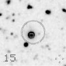
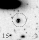
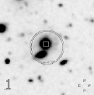
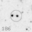
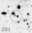
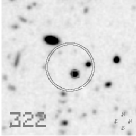
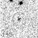
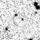
Figure 2.— (Upper panel): examples of I–band finding charts of sources with a unique optical counterpart or securely identified from the likelihood analysis. (Middle panel): examples of I–band finding charts of sources with ambiguous counterparts. (Lower panel): examples of K–band finding charts of sources identified from the K-band catalog. In all the panels, the circle is centered on the XMM–Newton position and has a radius of 5^′′.

Table 1Summary of optical identification of point-like X–ray sources

	all	identified		unidentified
Sources with I$<16$ (I bright)	21	21		-
Sources with I$>16$	674	587		87
Additional sources identified with K	-	46		-
Total	695	654		41
		reliable	ambiguous
		626	28

Fig. 1 shows the observed magnitude distribution of all optical objects present in the $I$ band catalog within a radius of 3″ around each X–ray source (solid histogram), together with the expected distribution of background objects in the same area, estimated using the procedure described above (dashed histogram). The difference between these two distributions (dotted histogram) is the expected magnitude distribution of the optical counterparts. The smooth curve fitted to this histogram (dotted curve) has been used as the input in the likelihood calculation q(m); the normalization of this curve has been set to 0.76, corresponding to the ratio between the integral of the q(m) distribution and the total number of the X–ray sources. For the threshold value in the likelihood ratio we adopted $LR_{\rm th}$=0.4, which maximizes the sum of sample reliability and completeness in the present sample (Sutherland & Saunders, 1992; Brusa et al., 2005).

Figure 3.— (Upper panel): Histogram of the distances between the X–ray and optical counterparts for all the 654 sources identified as discussed in Sect. 2.3 (solid histogram) and the subsample of sources with spectroscopic redshift and classification (shaded histogram). The inset in the top-right part of the plot shows the cumulative distribution of X–ray to optical distances for all the sources (bold curve) and for the subsample of sources with spectroscopic redshift (dashed curve). The dashed line at 3^′′ marks the radius which encloses 90% of the X–ray counterparts (see discussion in Section 2.2). (Lower panel): Histogram of the I-band magnitudes distribution for the 633 primary identifications fainter than I_AB=16. The solid and shaded histograms have the same meaning as in the upper panel. The dashed histogram shows the lower limit to the I_AB magnitudes, corresponding to the brightest objects in the error-circles, for the 41 X–ray sources without an optical identification. The inset in the top-right part of the plot shows the cumulative distribution of X–ray to optical distances for all the sources with I¿16 (bold curve) and for the subsample of sources with spectroscopic redshift (dashed curve).

Figure 4.— Redshift distribution for the sample of 243 sources with “secure” spectroscopic information from Magellan/IMACS data (Trump et al., 2007)), zCOSMOS project (Lilly et al., 2007) and from the SDSS archive (Adelman-McCarthy et al., 2005). The black filled histogram shows the contribution of spectroscopically classified Broad Line AGN. The redshift windows in which each broad line (H$\alpha$, H$\beta$, MgII, CIII], CIV) is visible in the IMACS/zCOSMOS spectra (wavelength range $\sim$5400-9000 Å) are also reported in the upper part of the Figure.

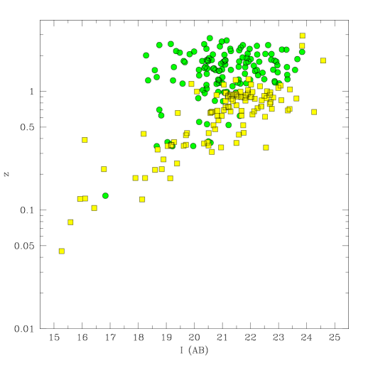
Figure 5.— Redshift versus I-band magnitude for sources spectroscopically classified as BL AGN (green circles) and NOT BL AGN (yellow squares).

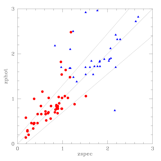
Figure 6.— Photometric redshifts versus spectroscopic redshifts for the sources with secure redshifts in the 12F sample. Red circles mark extended sources, blue triangles mark point-like objects, on the basis of the ACS data. The dotted lines limit the locus for which $|z_{spec}-z_{phot}|<0.15\times(1+z_{\rm spec})$

.

2.3. Results

We computed the likelihood ratio for all the optical sources within 7″ of the 674 X-ray centroids (a total of 2158 sources), finding 730 optical sources with LR$>$LR_th. The expected number of true identifications among these objects, computed by summing the reliability of each of them, is $\sim$524 ($\sim$78% of the total number of X-ray sources). The number of X-ray sources which have at least one optical source with LR$>$LR_th is 587 (87% of the sample). The remaining 87 X-ray sources either are associated with LR$<$LR_th counterparts (74) or do not have any optical counterpart in the catalog within 7″ from the X-ray centroids (13). We have therefore visually checked these 87 unidentified sources. In 24 cases we found a clear, relatively bright optical source within the X-ray error-circle in the I-band image. These objects were missing in the input CFHT catalog used to compute the likelihood ratio (mainly because close to bright objects and/or in CCD masked regions) or they were present but incorrectly associated with a much fainter magnitude. The I–band magnitudes of these 24 sources were therefore retrieved from the Subaru multicolor catalog, and added to our list of possible counterparts. It is important to note that this problem affects only a minority of the X–ray source counterparts ($\sim$3.5%, most of them close to bright stars and/or defects in the optical band images) and it can be easily solved with the adopted procedure.
We then ran the likelihood analysis again, this time using as input catalog the K-band (KPNO/CTIO) data extracted from the multicolor catalog (see Capak et al. 2007). The main advantage of using also this near-infrared catalog is due to the fact that the X-ray to near-infrared correlation for AGN is much tighter than the one in the optical bands (Mainieri et al., 2002; Brusa et al., 2005). Moreover, although the currently available K–band data are shallower than the optical ones, their use is potentially important to find the reddest optical counterparts, which are a not negligible fraction of the identifications of faint X–ray sources (see, e.g., Alexander et al. 2001).

Indeed, using this catalog and adopting the same value of LR_th=0.4, we found likely counterparts for 46 of the 87 unidentified sources, that include all the 24 discussed above and 22 additional red, faint sources with unambiguous identification in the K–band (see also Mignoli et al. 2004).
Summarizing, on the basis of the likelihood analysis applied to the I-band and K–band catalogs, we have possible counterparts for 633 out of 674 X-ray sources (654 out of 695 when the 21 sources brighter than I=16 are included). We have further tentatively divided the 654 proposed identifications in “reliable” and “ambiguous”. In the first class we include the 21 sources with I_AB$<$16, the 559 sources for which either there is only one object with LR$>LR_{\rm th}$ or the ratio between the highest and the second highest LR value in the I or K–band is greater than 3, and the 46 sources identified only in the K–band. The total number of objects in this class is therefore 626. The combined use of optical and NIR catalogs for the identification process led to a number of ”reliable” counterparts larger than that inferred from the use of the optical catalog only (524). However, we note that $\sim 5$% of these reliable counterparts can still be misidentifications. The other 28 sources comprise all the sources for which the ratio of LR values in the I– or K–band of the possible counterparts is smaller than 3, and they are considered as ambiguous. In the following we tentatively identify these 28 X–ray sources with the optical counterparts with the highest LR value.
Table 1 gives a summary of the identifications, while Figure 2 shows a few examples of finding charts for sources representative of the different types discussed above.

For the remaining 41 sources, the possible counterparts have on average faint or very faint optical magnitudes, none of them has LR$>$ LR_th, and most of them lie at $\Delta(X-O)>$2^′′. For a fraction of them the true counterpart of the X–ray source may indeed be very faint and/or undetected in the optical bands (see e.g. Koekemoer et al. 2004). Another possibility is that the X–ray emission originates from a group of galaxies at high-redshift with optically faint members: in this case, the X–ray extension of the putative group emission may be comparable to or smaller than the XMM–Newton PSF and the source can have been classified as point-like. Finally, a small fraction of these objects can be spurious X–ray sources, as suggested by the fact that the percentage of sources with low X–ray detection likelihood (e.g. DETML $<9$; see Cappelluti et al. 2007 for a definition of DETML) is significantly higher for these unidentified sources ($\sim 30$%) than for the optically identified X–ray sources ($\sim 10$%). A detection with Chandra  with significantly smaller error–circles, would definitively discriminate among these different possibilities.

2.4. Statistical properties

The distribution of the X-ray to optical distances and of the I-band magnitudes for the X–ray sources identified as described in Sect. 2.3 are shown in Fig. 3 (solid histograms). For the X-ray sources with more than one optical counterpart with LR$>$LR_th, the X-ray to optical distance and the I band magnitude of the optical object with the highest LR is plotted. In the lower panel the dashed histogram shows the lower limits to the I_AB magnitudes, corresponding to the brightest objects in the error circles, when the 41 X-ray sources without an optical identification are also added.
About 90% of the reliable optical counterparts have an X–ray to optical separation ($\Delta(X-O)$) smaller than $3^{\prime\prime}$ (see inset in the upper panel of Fig. 3), which is consistent with or even better than the $\sim 80$% within 3^′′ found in XMM–Newton data of comparable depth (see e.g. Fiore et al. 2003; Della Ceca et al. 2004; Loaring et al. 2005). The improvement is likely given by the combination of the accurate astrometry of the positions of the X-ray sources (tested with simulations in Cappelluti et al. 2007), and the full exploitation of the multiwavelength catalog (optical + K) for the identification process (that makes ”reliable” a larger number of sources). In addition, because of the geometry of the final mosaic, most of the X–ray sources are closer than 5’ to the center of at least one pointing, so that the corresponding PSF is not significantly deteriorated. The majority of the X-ray sources ($\sim$73%) have counterparts with I_AB magnitudes in the range $20<I_{\rm AB}<$24, with two tails at fainter ($\sim$12%) and brighter ($\sim$15%) magnitudes. The median magnitude of optical counterparts is I${}_{\rm AB}=$21.65.
These distributions do not change significantly if we make a different choice for the optical counterpart of the 28 “ambiguous” sources, i.e. the second most likely optical counterpart is considered. Therefore, from a statistical point of view the properties of these 654 X-ray sources (see Table 1) can be considered representative of the overall X-ray point source population, at the sampled X–ray fluxes.

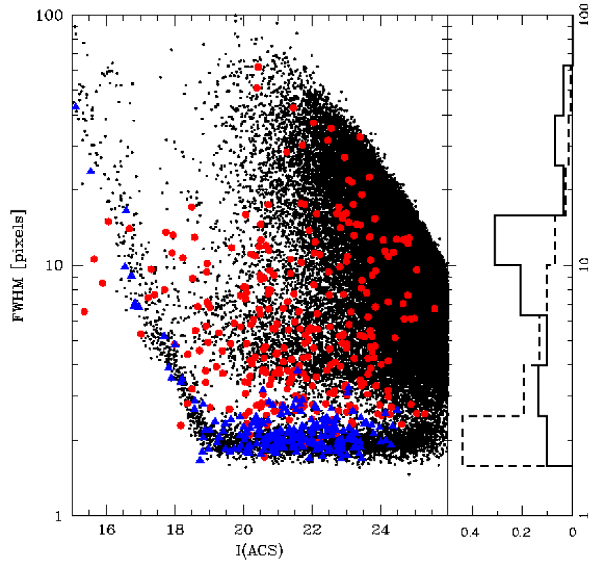
Figure 7.— Full Width Half Maximum (FWHM) vs. ACS I-band magnitude for all the sources (small black symbols) in the ACS photometric catalog. Overplotted as blue triangles (red circles) are the X-ray sources classified as point-like (extended) from ACS. The histograms on the right part of the figure show the distribution of FWHM for the sources detected only in the soft band (dashed histogram) and for the sources detected only in the hard band (solid histogram). Both histograms are normalized to the total number of sources in each class.

2.5. Redshift distribution

Spectroscopic redshifts for the proposed counterparts are available from the Magellan/IMACS observation campaign (193 objects, Impey et al. 2007; Trump et al. 2007) and the first run of zCOSMOS observations (25 objects, Lilly et al. 2007; J.P. Kneib, private communication) and/or were already present in the SDSS survey catalog (48 objects, Adelman-McCarthy et al. 2005; Kaufmann et al. 2003), for a total of 248 independent redshifts (five of them of galactic stars). Spectroscopic information and classification is therefore available for a substantial fraction of our optical/infrared counterparts (248/654, $\sim$38%). The X–ray to optical distances and the I–band magnitude distributions of the subsample with spectroscopic redshift are shown as shaded histograms in both panels of Fig. 3. The spectroscopic completeness is $\sim$50% at I${}_{\rm AB}\leq$22 and drops to $\sim$35% at 22$<$ I${}_{\rm AB}\leq$23 and to $\sim$18% at 23$<$ I${}_{\rm AB}\leq$24.
While a more detailed analysis of the optical spectra will be presented in future papers, based also on more data that are rapidly accumulating from the on-going projects, for the purposes of the present paper we divided the extragalactic sources (243 objects) in only two classes, following Fiore et al. (2003): objects with broad optical emission lines (BL AGN, 126 in total) and sources without a clear, broad emission signature in the optical band, but with narrow emission or absorption lines (NOT BL AGN, 117). The latter class is therefore a mixed bag of different types of objects, and comprises mainly narrow-lined AGN, low-luminosity AGN, starbursts and normal galaxies. Figure 4 shows the redshift distribution for all the extragalactic sources in the spectroscopic sample (solid empty histogram) along with the redshift distribution of the sources spectroscopically classified as BL AGN (filled histogram). At low redshift (z$<$1) the spectroscopic identifications are dominated by objects associated with NOT BL AGN, while at high redshifts (z$>$1.5) almost exclusively BL AGN are detected. As already noted by Eckart et al. (2006) and Cocchia et al. (2007), the small number of narrow line objects at z$>$1.5 is most likely due, at least in part, to selection effects: high-redshift narrow line AGN are on average fainter in the I-band than BL AGN and a significant fraction of them is expected to be below the optical magnitude limit for spectroscopic follow-up. This is shown in Fig. 5, where the spectroscopic redshifts are plotted versus the I–band magnitudes of the optical counterparts, for both BL AGN (green circles) and NOT BL AGN (yellow squares): while BL AGN show a large spread in I magnitudes over a large redshift range, the distribution of NOT BL AGN in this plane is much narrower and shows a rapid rise in I magnitude with redshift (see also Fig. 14 in Trump et al. 2007 paper). Conversely, the small number of BL AGN at low-z can be ascribed to several factors: 1) spectroscopic misclassification: given the wavelength range ($\sim$5400-9000 Å) of both the IMACS and the VIMOS zCOSMOS data, at low redshift (z $\mathrel{\hbox to0.0pt{\lower 3.0pt\hbox{$\mathchar 536\relax$}\hss}\raise 2.0pt\hbox{$\mathchar 316\relax$}}$1) broad emission lines are not well sampled (e.g. H$\alpha$ is not visible at z$\mathrel{\hbox to0.0pt{\lower 3.0pt\hbox{$\mathchar 536\relax$}\hss}\raise 2.0pt\hbox{$\mathchar 318\relax$}}0.4$, H$\beta$ is not visible at z$\mathrel{\hbox to0.0pt{\lower 3.0pt\hbox{$\mathchar 536\relax$}\hss}\raise 2.0pt\hbox{$\mathchar 318\relax$}}0.8$ and MgII enters the spectral window at z$\sim$1), while narrow lines (e.g. [OII]) and/or absorption features (e.g. Balmer break) can be more easily detected; 2) especially in the case of moderately weak Seyferts, the relative contribution of the host galaxy and the AGN can be such that the broad lines are diluted in the stellar light and can be revealed only in high S/N spectra (Moran, Filippenko & Chornock, 2002; Severgnini et al., 2003).

To obtain a complete redshift distribution for the X–ray sources, photometric redshifts should be computed for the sources without spectroscopic data. As a training sample, we used the code described in Bender et al. (2001) and tested it on the sample of objects with secure spectroscopic redshifts. For objects classified as “extended” in the ACS images (see Section 3.1), we applied the same semi–empirical templates of non–active galaxies that have been used to compute the photometric redshift in the Fornax Deep Fields (see Gabasch et al. 2004 and references therein) and GOODS-South field (Salvato et al., 2006); in both applications, a $\sigma$($\Delta z/(1+z)$) $\sim$0.05 has been obtained. For objects that have been classified as point-like sources, only AGN templates have been adopted (see also Mainieri et al. 2005 and reference therein). In Fig. 6 our best attempt so far is shown. Red circles are optically extended X-ray selected sources, while blue triangles represent point-like objects. A relatively high fraction of both extended ($\sim$73%) and point-like ($\sim$66%) sources have $|z_{spec}-z_{phot}|<0.15\times(1+z_{\rm spec})$.

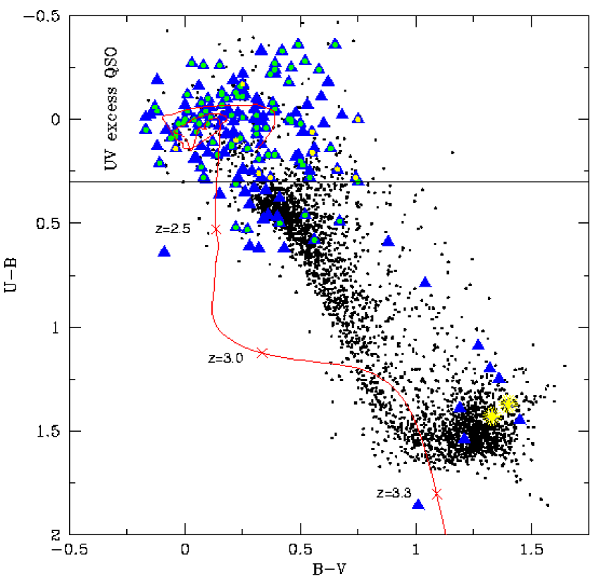
Figure 8.— U-B vs. B-V diagram for all the fields objects with B$>19$ (small black points) classified as point-like in the full ACS catalog and with an error in all the three optical bands smaller than $<0.15$ (Capak et al., 2007). The locus occupied by stars is clearly defined in this diagram, with the two densely populated regions in the blue (upper left of the black points envelope; hot subdwarf stars) and red (lower right; dwarf M stars) parts of the sequence. The horizontal solid line marks the color cut for the selection of ultraviolet excess objects. Overplotted as blue triangles are the counterparts of X–ray sources classified as point-like from ACS, which satisfy the same selection in the photometric errors. Spectroscopically confirmed BL AGN and NOT BL AGN are also indicated (green and yellow symbols overplotted on the blue ones, respectively). Finally, the expected tracks of quasars from redshift 0 to $\sim$3.5 in this color-color diagram is also reported (see text for further details).

3. Multiwavelength properties

3.1. ACS morphology: stellar vs. extended objects

The catalog of the primary optical counterparts of the X–ray sources was then cross-correlated with the June 2005 version of the ACS catalog (Leauthaud et al., 2007; Koekemoer et al., 2007), from the first HST cycle (Cycle 12), in order to gather some preliminary information on the morphological classification of the X-ray sources. Since the available ACS catalog does not cover the entire XMM-COSMOS area analyzed here, we could use ACS information only for 524 optical sources, out of the total of 654. For these sources, we retrieved from the catalog the measure of the Full Width Half Maximum (FWHM, in image pixels), the ACS I–band magnitude and a parameter that defines the morphological classification (stellar or extended) on the basis of the analysis of the available data. Following Leauthaud et al. (2007), objects were divided in “stellar/point-like” (hereinafter: point-like) and “optically extended”’ (hereinafter: extended) on the basis of their position in the plane defined by the peak surface brightness above the background level and the total magnitude (see Fig. 6 in Leauthaud et al. 2007). The FWHM versus the I-band magnitude is shown in Fig. 7; in this figure, the blue triangles indicate sources classified as “point-like”, and red circles sources classified as “extended”. More than 50% of the primary IDs have stellar (or almost stellar; FWHM $<$ 3 pixels) profile on ACS data. This is particularly true for the very soft sources (i.e. detected only in the soft band, see dashed histogram in Fig. 7). The situation is completely different for the really hard sources (i.e. no detection in the soft band, solid histogram in Fig. 7), for which most of the counterparts ($\sim$80%) are associated with extended sources.
A subsample of 214 objects (108 BL AGN, 101 NOT BL AGN, 5 stars) has both spectroscopic information and ACS classification. In agreement with the expectations, we find a good correspondence between ACS and spectroscopic classification: the majority of BL AGN are classified as point-like by ACS (86/108, $\sim$80%), while the majority of NOT BL AGN are classified as extended by ACS (85/101, $\sim$85%). A total of 38 sources show a “mismatch” between the morphological and spectroscopic classification and we will come back to these sources later in the paper.

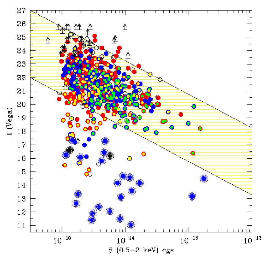
Figure 9.— The I-band magnitude (Vega system) vs. the soft (0.5-2 keV) flux for all the primary counterparts in the sample (all symbols), and the subsamples of objects classified as point-like (blue circles) and extended (red circles) from ACS morphology. The shaded area represents the region typically occupied by known AGN (e.g. quasars and Seyferts) along the correlation log$(X/O)=0\pm 1$. Spectroscopically confirmed BL AGN and NOT BL AGN are also indicated (green and yellow symbols, respectively). Asterisks mark the objects tentatively identified with stars (see Sect. 3.2 and 3.3). Lower limits to the I band magnitude correspond to the magnitude of the brightest objects in the error-circles of the unidentified X–ray sources.

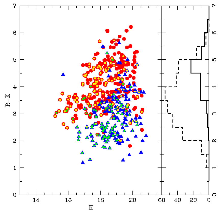
Figure 10.— R-K color vs. K band magnitude (Vega system) for the X-ray sources counterparts with ACS information. Symbols as in Fig. 9. Sources spectroscopically identified with BL AGN (green) and NOT BL AGN (yellow) are also highlighted. The histogram on the right part of the figure shows the distribution of R-K colors for the sources with HR$>-0.3$ (i.e. candidate X–ray obscured AGN, solid histogram) and the sources detected only in the soft band (HR=$-1$, dashed histogram).

3.2. Optical color-color diagrams for point-like objects

Figure 8 shows the U-B vs. B-V diagram for all field objects (small black points) with B$>$19 classified as point-like in the full ACS catalog and with an error in all the three optical bands smaller than 0.15 magnitude (Capak et al., 2007). The locus occupied by stars is very well defined in this diagram, with the two densely populated regions in the blue (upper left of the black points envelope; hot subdwarf stars) and red (lower right; dwarf M stars) parts of the sequence. Most of the points at U-B$<$0.3 (UVX objects) are expected to be AGN at z$\mathrel{\hbox to0.0pt{\lower 3.0pt\hbox{$\mathchar 536\relax$}\hss}\raise 2.0pt\hbox{$\mathchar 316\relax$}}$2.3, while the objects on the right of the stellar sequence are likely to be compact galaxies classified as point-like. Overplotted as blue triangles are the X–ray sources classified as point-like from ACS which satisfy the same selection in the photometric errors. Spectroscopically confirmed BL AGN and NOT BL AGN are also indicated (following Fig. 5, green and yellow symbols overplotted on the blue ones, respectively). Finally, the expected track of quasars from redshift 0 to 3.5 in this color-color diagram is also reported, computed using the SDSS AGN template from (Budavari et al. 2001; see also Capak et al. 2007 for further details).
It is quite reassuring that the majority ($\mathrel{\hbox to0.0pt{\lower 3.0pt\hbox{$\mathchar 536\relax$}\hss}\raise 2.0pt\hbox{$\mathchar 318\relax$}}80$%) of X-ray selected point-like quasars occupy the classical QSO locus and would have been selected as outliers from the stellar locus in this color-color plot. A few (5 to 8) sources are within or close to the locus of “red” stars. So far we have spectroscopic data only for two of these objects and both of them are stars. All these sources are detected only in the soft X-ray band and show a low ($<$0.1) X-ray to optical flux ratio (X/O) and are therefore likely to be stars. A similar number (8 to 10) of X-ray sources are within or close to the locus of blue stars. The spectroscopic identifications available for these objects include three BL AGN at z$\geq 1.4$; a fourth object is likely to be a star on the basis of the bright I band magnitude and low X/O ratio.

3.3. X–ray to optical flux ratio

Another independent check on the agreement between optical identification, morphological analysis and spectroscopic breakdown is shown in Fig. 9, where the I-band magnitude (Vega system) is plotted versus the soft X-ray flux for all the X-ray sources (black empty symbols), ACS-point-like objects (blue symbols) and ACS-extended sources (red symbols).
As discussed in Sect 2.1, the sources brighter than I_AB=16 are identified “a priori”: all of them have been visually inspected and the majority of them turned out to be associated with bright stars and have point-like morphology from ACS. A sample of 8 additional stars has been tentatively identified on the basis of the information from U$-$B vs. B$-$V diagram, the bright optical magnitudes and the low X–ray to optical flux ratio. All the sources identified with stars (a total of 25) are plotted as asterisks in Fig. 9 and they constitute $\sim$4% of the soft X–ray selected sample. This value is similar to that reported in the ROSAT Deep Survey (Lehmann et al., 2001) and in the ChaMP survey (Green et al., 2004), from the optical identification of large samples (100–300) of soft X–ray selected sources at limiting fluxes similar to that of COSMOS.

If objects associated with stars are removed, point-like sources occupy preferentially the locus in this plane with X/O in the range 0.1$\div$10, where most of the broad line quasars from previous optical and soft X–ray selected surveys lie (hatched region in Fig. 9). Also most of the extended sources are within the same range of X/O ratio, but with more significant tails toward both low and high values of X/O. For most of these sources, thanks to the superb ACS resolution, it will be possible to resolve the nucleus and the host galaxy. Optically bright (i.e. X/O$<$0.1) extended sources are preferentially identified with nearby galaxies, in which the optical luminosity is mainly due to the integrated stellar light; for the majority of them, the high-level of observed X–ray flux suggests that some activity is taking place in their nuclei (see, e.g. Comastri et al. 2002).

3.4. Optical to near-infrared colors

Figure 10 shows the R$-$K vs. K–band magnitude (Vega magnitudes) for the subsample of objects with ACS morphological information (excluding spectroscopically confirmed stars). In addition, sources spectroscopically identified with BL AGN are marked with green symbols, while sources identified with NOT BL AGN are marked by yellow symbols. A significant difference in the R$-$K distributions for point-like and extended sources is present : while the widths of the two distributions are similar ($\sigma\sim$0.8 for both of them), extended sources are significantly redder ($\langle R-K\rangle$=4.05$\pm 0.05$) than point-like sources ($\langle R-K\rangle$=2.91$\pm 0.06$). When the spectroscopic information is also considered, objects with red $R-K$ colors are preferentially associated with NOT BL AGN (yellow circles), while blue objects are preferentially associated with BL AGN (green circles).

We have then investigated the distribution of the $R-K$ colors as a function of the X–ray hardness ratio (HR), a widely used tool to study the general X-ray spectral properties of X-ray sources when the number of counts is inadequate to perform a spectral fit. Mainieri et al. (2007) (paper IV of this series) have shown that 99% of the sources with HR$>-0.3$ in their subsample can be fit by a $\Gamma$=1.8-2 power-law continuum absorbed by a column density (N_H) larger than $10^{22}$ cm^-2. Conversely, sources detected only in the soft band (i.e. HR=-1) are most likely unobscured.
The hardest sources (HR$>-0.3$, solid histogram in the right part of Fig. 10) are mostly associated with red and very red objects (R-K$>$4). This indicates an excellent consistency between optical obscuration of the nucleus as inferred from ACS (extended morphology), optical to near infrared colors, and the presence of X–ray obscuration as inferred from the hardness ratio (see also Alexander et al. 2001; Giacconi et al. 2002; Brusa et al. 2005; Mainieri et al. 2007). Conversely, sources detected only in the soft band (i.e. HR=$-1$, dashed histogram) have preferentially blue R-K colors ($>60\%$ of the sources have $R-K<4$), typical of those of optically selected, unobscured quasars (Barkhouse & Hall, 2001). It is interesting to note, however, that the observed correspondence between hard (soft) X–ray colors and red (blue) optical to near infrared colors is not a one-to-one correlation (see also, e.g., Georgantopoulos et al. 2004; Brusa et al. 2005). In fact, as shown for example by the tail toward high R-K colors of the dashed histogram in Fig. 10, a non-negligible fraction of red objects is associated with very soft X–ray sources.

Figure 11.— Distribution of the absolute B–band magnitude for BL AGN (solid histogram, upper panel) and NOT BL AGN (solid histogram, lower panel) in the subsample of objects with ACS information and spectroscopic classification. In both panels the shaded histograms give the contribution of outliers in each class, i.e. “extended” BL AGN and “point–like” NOT BL AGN, respectively. The dashed line at M_B=-23 marks the “classic” separation between Seyfert and Quasars.

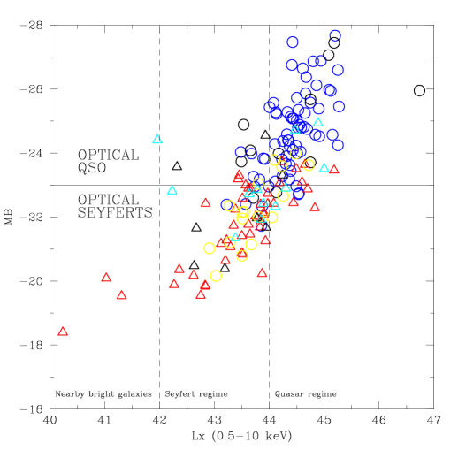
Figure 12.— Absolute rest frame B-band magnitude vs. the logarithm of the full (0.5-10 keV) X–ray luminosity (erg s^-1). Symbols are as follows: Blue circles = spectroscopically confirmed BL AGN classified as point-like from ACS; Yellow circles = spectroscopically confirmed BL AGN classified as extended from ACS; Cyan triangles = spectroscopically confirmed NOT BL AGN classified as point-like from ACS; Red triangles = spectroscopically confirmed NOT BL AGN classified as extended from ACS. The horizontal solid line marks the “classic” optical transition between Seyfert and Quasars.

3.5. Outliers: mismatch between morphological and spectroscopic classification

As discussed in Sect. 3.1, there is a relatively good agreement (of the order of 80%) between the morphological and spectroscopic classifications for the subsample of sources for which these informations are available. However, there are 22 ($\sim 20$%) BL AGN classified as “extended” in ACS and 16 ($\sim 16$%) NOT BL AGN classified as point-like by ACS.
The absolute magnitude is an obvious quantity to examine in order to try to understand why for these sources the morphological and spectroscopic classifications do not agree with each other. Figure 11 shows the distribution of rest–frame, absolute B–band magnitude for the 209 extragalactic sources which have both morphological (ACS) and spectroscopic classification, separately for BL AGN (upper panel) and NOT BL AGN (lower panel). The black filled histograms show the observed distribution for the “outliers”, i.e. “extended” BL AGN and “point-like” NOT BL AGN, respectively. In order to minimize the uncertainties in the K-correction, the absolute B–band magnitudes have been computed from the apparent magnitude in the optical filter closest to the rest-frame B band at any given redshift.
All the “extended” BL AGN lie at redshift $<$1.5, while the redshift distribution of the full BL AGN population peaks at z$\sim$1.5 (see Figg. 4 and 5). The fact that ACS reveals an extended component is likely to be due to the fact that the nuclear emission in these objects is not dominant with respect to the host galaxy emission, at least in the observed ACS band. Indeed, the average M_B of the extended BL AGN sources lies in the low-tail of the M_B distribution of the entire BL AGN population and typically in the Seyfert regime, taking M${}_{B}=-23$ as the “classical” separation between Seyferts and QSO (Schmidt & Green, 1983).
The unresolved nature of “point-like” NOT BL AGN is more puzzling. It can be due, at least in part, to the definition we adopted for the segregation of stellar objects: especially at high redshift, the ratio between the peak flux and the total magnitude cannot be such to define them ”extended”. However, we note that most of them occupy the high-luminosity tail of the distribution of M_B of the overall population of NOT BL AGN, and therefore can be classified as high-luminosity, type 2 quasars from the available optical spectroscopy (see also Mainieri et al. 2007 for a more detailed analysis of the rest–frame X–ray properties). Moreover, they tend to be “bluer” (i.e. less absorbed) in the optical to near infrared colors (yellow symbols on blue points in Fig. 10), suggesting that we are seeing more directly the emitting nucleus.

Fig. 12 shows the absolute B magnitude as a function of the 0.5-10 keV luminosity (as computed in Mainieri et al. 2007) for the subsample of sources with spectroscopic redshift and good X–ray counting statistics. Circles mark BL AGN (blue for the point-like and yellow for the extended sources) while triangles mark NOT BL AGN (cyan for the point-like and red for the extended sources). Sources with L${}_{X}<10^{42}$ erg s^-1 are mostly associated with bright (I$<$18), extended objects (red triangles) at z$<$0.2; two of them are detected only in the soft band. Among the two sources detected also at higher energies, there is source the candidate Compton Thick AGN discussed in Hasinger et al. (2007).
The region at luminosities higher than 10⁴⁴ erg s^-1 is mainly populated by point-like, BL AGN (blue circles). Only 8 sources classified as NOT BL AGN lie in this part of the diagram: the high X–ray luminosity classifies them as candidate Type 2 QSO (Mainieri et al., 2007). Conversely, the majority of the sources in the middle part of the X–ray luminosity region are associated with extended, NOT BL AGN (red triangles) and low redshifts BL AGN (Seyfert 1 galaxies, yellow circles).

4. Discussion

Comparing the optical color-color properties of AGNs in the COSMOS field with those of field objects (see Fig. 8), we estimate that X–ray data with a flux limit of S${}_{\rm 0.5-2keV}\sim 10^{-15}$ erg cm^-2 s^-1 recover at least half (50%) of the AGN candidates which would be selected on the basis of their ultraviolet excess (U-B$<$0.3) at B$\mathrel{\hbox to0.0pt{\lower 3.0pt\hbox{$\mathchar 536\relax$}\hss}\raise 2.0pt\hbox{$\mathchar 316\relax$}}$23 (see Zamorani et al. 1999 for a similar estimate at a somewhat brighter X–ray flux from ROSAT observations in the Marano field). This fraction of 50% has been obtained assuming that all objects with ultraviolet excess are AGN. Since at these magnitudes blue stars and compact galaxies may represent $\sim 30$% of the samples of point–like objects with ultraviolet excess (Mignoli & Zamorani, 2001), we conclude that the efficiency of present X–ray data in detecting AGN with ultraviolet excess at B$\leq$23 is likely to be as high as 70%. We note that the large majority of the BL AGN selected via the UV excess method have MB$<-23$ (see Fig. 11) and are therefore classified as quasars, confirming previous results (see e.g Zamorani et al. 1999 and reference therein). We also note, however, that the photometric catalog we use has deeper limiting magnitudes with respect to all the previous studies on optically selected UV-excess QSO and therefore we start to explore and pick up lower-luminosity (e.g. Seyfert-like) objects up to z$\sim 1.5$. On the other hand, a significant fraction ($\sim$40%) of the X-ray selected AGNs, especially those without broad lines in their optical spectra, would have not been easily selected as AGN candidates on the basis of purely optical criteria, either because of colors similar to those of normal stars or field galaxies at z$\sim$1-3, or because of morphological classification not consistent with that of point–like sources (see Fig. 10). These results highlight the need for a full multiwavelength coverage to properly study and characterize the AGN population as a whole.
With the current spectroscopic coverage ($\sim$38%) the observed redshift distribution and spectroscopic classification of identified X–ray sources could be biased against low-redshift BL AGN and high-redshift NL AGN (see Sect. 2.5 and Trump et al. 2007 for a more detailed discussion on AGN selection effects in COSMOS; see also Treister et al. 2004). However, according to the most recent modeling of the X–ray luminosity function evolution (e.g. Ueda et al. 2003; Barger et al. 2005; Hasinger, Miyaji & Schmidt 2005; La Franca et al. 2005), the paucity of low-redshift BL AGN and high–redshift obscured NL AGN may be at least partly real and due to a luminosity dependent evolutionary behaviour of X–ray selected sources. The space density of high luminosity (L${}_{\rm X}>10^{44}$ erg s^-1) quasars decreases steeply below z$\simeq$1, while the decrease of the space density of lower luminosity objects in the same redshift range is much slower (see, e.g., Fig. 9 in Fiore et al. 2003). Moreover, there are now increasing evidences that the relative ratio between obscured and unobscured AGN is a decreasing function of the X–ray luminosity (Ueda et al., 2003; Hasinger, 2004; La Franca et al., 2005; Akylas et al., 2006). As a consequence, at low redshifts the X–ray source population is dominated by low luminosity, often obscured AGN, while at higher redshifts luminous unobscured quasars take over. This is in qualitative agreement with the observed change of the Type 2/ Type 1 ratio (R) in the present sample when the typical Seyferts (32/33, R$\sim$1 at L${}_{X}\sim 10^{42}-10^{44}$ erg s^-1) and Quasars (8/44, R$\sim$0.18 at L${}_{X}>10^{44}$ erg s^-1) luminosities are considered (see Fig. 12).

At a limiting flux of 2$\times 10^{-15}$ erg cm^-2 s^-1 in the soft band, where the sky coverage has decreased to 50% of the total 1.3 deg² area covered by the 12F pointings, no object at z$>$3 is present so far in our current spectroscopic sample. On the one hand, the lack of high redshift sources could be due, at least in part, to the still limited spectroscopic completeness, which is of the order of 50% at I_AB$<$22 and about 25% at fainter magnitudes, with no spectroscopic redshifts for I_AB$>$24. As a comparison, Murray et al. (2005) have 14 z$>3$ quasars in their 9 deg² X-Bootes survey, at a limiting flux about one order of magnitude brighter than our survey and with a similar spectroscopic completeness. By rescaling the area and the limiting fluxes, this would translate in $\sim 3$ z$>3$ quasars in the XMM-COSMOS 12F area, that is still consistent with zero being observed. On the other hand, the number of AGN at z$>$3 expected from population synthesis models (see also Hasinger et al. 2007; Gilli, Comastri & Hasinger 2007) is $\sim$30 and a random sampling at $\sim$25% completeness, to take into account the current follow-up spectroscopy, would therefore predict about 7 quasars at z$>$3, which are not observed. The forthcoming spectroscopic observations will increase the spectroscopic completeness, allowing to verify if a sizable number of high redshift (z$>$3) quasars is present among the optically faintest counterparts and among the optically unidentified X–ray sources, or if some of the model assumptions, mainly based on extrapolations of the lower redshift (z$<3$) luminosity functions, should be refined.

5. Summary

In this paper we presented the optical identifications for a large subsample ($\sim$700) of X–ray sources detected in the first 1.3 deg² of the XMM-COSMOS observations, down to a 0.5-2 keV limiting flux of $\sim 10^{-15}$ erg cm^-2 s^-1. The X-ray counterparts have been identified in optical (I–band) and near infrared (K–band) catalogs, making use of the “maximum likelihood” technique. The combined use of the two different catalogs allowed us to test the identification procedure and turned out to be extremely useful both for isolating input catalogs problems and for identifying optically faint counterparts. Overall, 90% (626) of the X–ray sources have been unambiguously associated with optical or near–infrared counterparts. Twenty eight X–ray sources have 2 possible optical counterparts with comparable likelihood of being the correct identification. These sources have been classified as “ambiguous” and we tentatively identify them with the optical counterpart with the highest LR value. The sample of proposed identifications therefore comprises 654 objects, while for the remaining 41 X–ray sources it was not possible to assign a candidate counterpart. We will use the forthcoming Chandra data (granted in AO8) to definitively discriminate the ambiguous and false associations and we also predict that a large fraction of these very faint, unidentified objects will be resolved with the inclusion of Spitzer (IRAC and MIPS) data in the source identification.
We then cross-correlated our proposed optical counterparts with the Subaru multi-color catalog (Capak et al., 2007), the HST/ACS data (Leauthaud et al., 2007) and the first results from the massive spectroscopic campaigns in the COSMOS field (Trump et al., 2007; Lilly et al., 2007). Our analysis reveals that for $\sim$80% of the X–ray sources counterparts with spectroscopic redshifts (a total of 248) there is a good agreement between the spectroscopic classification, the morphological parameters, and optical to near infrared colors: the large majority of spectroscopically identified BL AGN have a point-like morphology on ACS data (see Sect. 3.1), blue optical colors in color-color diagrams (see Sect. 3.2), and an X–ray to optical flux ratio typical of optically selected quasars (see Sect. 3.3). Conversely, NOT BL AGN are on average associated with extended optical sources, have significantly redder optical to near infrared colors and span a larger range of X–ray to optical flux ratios (see Sect. 3.3 and 3.4). When the X–ray information is also considered, we found that hard X–ray sources are preferentially associated with extended sources and are “reddish” ($\sim$60% with R-K$>$4, see also Mainieri et al. 2007), while sources detected only in the soft band are mostly associated with point-like objects and have “blue” optical to near–infrared colors.
Comparing the optical color-color properties of AGNs in the COSMOS field with those of field objects (see Fig. 8), we estimate that X–ray data with a flux limit of S${}_{\rm 0.5-2keV}\sim 10^{-15}$ erg cm^-2 s^-1 recover $\sim 70$% of the AGN selected on the basis of their ultraviolet excess at B$\mathrel{\hbox to0.0pt{\lower 3.0pt\hbox{$\mathchar 536\relax$}\hss}\raise 2.0pt\hbox{$\mathchar 316\relax$}}$23. This fraction will rise up to (90-100)% at S${}_{\rm 0.5-2keV}\sim 5\times 10^{-16}$ erg cm^-2 s^-1, the final depth of the XMM–COSMOS survey.
About 20% of the sources show an apparent mismatch between the morphological and spectroscopic classifications. Our analysis indicates that, at least for BL AGN, the observed differences are largely explained by the location of these objects in the redshift–luminosity plane (see sect. 3.5). Our analysis also suggests a change of the Type 2/Type 1 ratio as a function of the X–ray luminosity, in qualitative agreement with the results from X–ray spectral analysis (Mainieri et al., 2007) and the most recent modeling of the X–ray luminosity function evolution (Figg. 5 and 12).
Although the Magellan/IMACS and VIMOS/zCOSMOS spectroscopic campaigns will continue to obtain redshifts for AGN in the COSMOS field, we expect that a fraction of the order of 30% of the sources will not have spectroscopic redshifts, due to the faintness of their optical counterparts ($\sim 15$%) and the limitation of multi-slit spectroscopy due to mask efficiency (Impey et al., 2007). We have tested a photometric code specifically designed to obtain redshifts for X–ray selected sources on the subsample of sources with spectroscopic data, and showed that it is possible to obtain a reasonable estimate of the sources redshifts ($|z_{spec}-z_{phot}|<0.15\times(1+z_{\rm spec})$), for $\sim$70% of the sources. We plan to use the same code to derive the redshifts for the faintest X–ray counterparts.

Summarizing, we were able to perform a combined multicolor, spectroscopic and morphological analysis on a statistical and meaningful sample of X–ray sources, and this work represents one of the most comprehensive multiwavelength studies to date of the sources responsible of most of the XRB (see also Eckart et al. 2006). This work is just the first phase of COSMOS AGN studies; the results presented in this paper clearly show the need for a full multiwavelength coverage to properly study and characterize the AGN population as a whole. As more data will become available, the selection of COSMOS AGNs by all available means - X-ray, UV, optical, near-IR, and radio - will build up to give the first bolometric selected AGN sample, fulfilling the promise of many years of multi-wavelength studies of quasars.

References

- Adelman-McCarthy et al. (2005) Adelman-McCarthy, J.K., Agüeros, M.A., Allam, S.S. et al., 2006, ApJS, 162, 38
- Akylas et al. (2006) Akylas, A., Georgantopouls, I., Georgakakis, A., Kitsionas, S. & Hatziminaoglou, E., 2006, A&A, in press, [astro-ph/0606438]
- Alexander et al. (2001) Alexander, D.M., Brandt, W. N., Hornschemeier, A.E., Garmire, G.P., Schneider, D.P., Bauer, F.E., & Griffiths, R.E., 2001, AJ, 122, 2156
- Alexander et al. (2003) Alexander, D.M., Bauer, F.E., Brandt, W.N., et al. 2003, AJ, 126, 539
- Barger et al. (2003) Barger, A.J., Cowie, L.L., Capak, P., et al. 2003, AJ, 126, 632
- Barger et al. (2005) Barger, A.J., Cowie, L. L., Mushotzky, R., et al. 2005, AJ, 129, 578
- Barkhouse & Hall (2001) Barkhouse, W.A., & Hall, P.B., 2001, AJ, 121, 2843
- Bender et al. (2001) Bender, R., Appenzeller, I.. Böhm, A. et al. 2001, Deep Fields, Proceedings of the ESO/ECF/STScI Workshop, Stefano Cristiani, Alvio Renzini, Robert E. Williams (eds.). Springer, 2001, p. 96.
- Brand et al. (2006) Brand, K., Brown, M.J., Dey, A., et al., 2006, ApJ, 641, 140 ARAA, 43, 827
- Brandt & Hasinger (2005) Brandt, N.W. & Hasinger, G., 2005, ARAA, 43, 827
- Brusa et al. (2005) Brusa, M., Comastri, A., Daddi, E., et al. 2005, A&A, 421, 69
- Budavari et al. (2001) Budavari, T., Csabai, I., Szalay, A.S., et al. 2001, AJ, 121, 3266
- Capak et al. (2007) Capak, P., et al. 2007, ApJS, this volume
- Cappelluti et al. (2007) Cappelluti, N., Hasinger, G., Brusa, M., et al., 2007, ApJS, this volume
- Ciliegi et al. (2003) Ciliegi, P., Zamorani, G., Hasinger, G., Lehmann, I., Szokoly, G., & Wilson, G. 2003, A&A, 398, 901
- Cocchia et al. (2007) Cocchia, F., Fiore, F., Vignali, C. et al. 2007, A&A in press, astro-ph/0612023
- Comastri et al. (2002) Comastri, A., Mignoli, M., Ciliegi, P., et al., 2002, ApJ, 571, 771
- Della Ceca et al. (2004) Della Ceca, R., Maccacaro, T., Caccianiga, A., et al., 2004, A&A, 428, 383
- Di Matteo et al. (2005) Di Matteo, T., Springel, V., & Hernquist, L., 2005, Nature, 433, 604
- Eckart et al. (2006) Eckart, M.E., Stern, D., Helfand, D.J., et al., 2006, ApJS, 156, 35
- Elvis et al. (1994) Elvis, M., Wilkes, B.J., McDowell, J.C., et al. 1994, ApJS, 95, 1
- Elvis, Risaliti, & Zamorani (2002) Elvis, M., Risaliti, G., & Zamorani, G., 2002, ApJ, 565, L75
- Fabian & Iwasawa (1999) Fabian, A.C. & Iwasawa, K., 1999, MNRAS, 303, L34
- Fabian (2004) Fabian, A.C., 2003, in ”Coevolution of Black Holes and Galaxies”, Carnegie Observatories Astrophysics Series, Vol. 1, ed. L.C. Ho (Cambridge Univ. Press), p. 447
- Ferrarese & Merritt (2000) Ferrarese, L., & Merrit, D., 2000, ApJ, 539, L9
- Finoguenov et al. (2007) Finoguenov, A., Guzzo, L., Hasinger, G., et al. 2007, ApJS, this volume, astro-ph/0612360
- Fiore et al. (2003) Fiore, F., Brusa, M., Cocchia, F. et al. 2003, A&A, 409, 79
- The First XMM-Newton Serendipitous Source Catalogue: 1XMM User Guide to the Catalogue (2003) The First XMM-Newton Serendipitous Source Catalogue: 1XMM User Guide to the Catalogue, Release 1.2 15 April 2003, Associated with Catalogue version 1.0.1, Prepared by the XMM-Newton Survey Science Centre Consortium [http://xmmssc-www.star.le.ac.uk/]
- Gabasch et al. (2004) Gabasch, A., Salvato, M., Saglia, R.P., et al., 2004, ApJ, 616, L83
- Gebhardt et al. (2000) Gebhardt, K., Kormendy, J., Ho, L., et al. 2000, ApJ, 543, L5
- Georgakakis et al. (2006) Georgakakis, A., Nandra, K., Laird, E.S., et al., 2006, MNRAS, 371, 221
- Georgantopoulos et al. (2004) Georgantopoulos, I., Georgakakis, A, Akylas, A., Stewart, G.C., Giannakis, O., Shanks, T., & Griiffiths, R.E., 2004, MNRAS, 352, 91
- Giacconi et al. (2002) Giacconi, R., Zirm, A., Wang, J., et al. 2002, ApJS, 139, 369
- Gilli, Comastri & Hasinger (2007) Gilli, R., Comastri, A., & Hasinger, G. 2007, A&A, in press, astro-ph/0610939
- Green et al. (2004) Green, P., Silverman, J.D.,, Cameron, R.A., et al. 2004, ApJS, 150, 43
- Hasinger et al. (2001) Hasinger, G., Altieri, B., Arnaud, M., et al. 2001, A&A, 365, L45
- Hasinger (2004) Hasinger, G., 2004, NuPhS, 132, 86
- Hasinger, Miyaji & Schmidt (2005) Hasinger, G., Miyaji, T., & Schmidt, M., 2005, A&A, 441, 417
- Hasinger et al. (2007) Hasinger, G., Cappelluti, N., Brunner, H. et al., 2007, ApJS, this volume, astro-ph/0612311
- Impey et al. (2007) Impey, C.D., Trump, J.R., McCarthy, P.J., et al. 2007, ApJS, this volume
- Kaufmann et al. (2003) Kauffmann, G., Heckman, T., Tremonti, C., et al., 2003, MNRAS, 346, 1055
- Koekemoer et al. (2004) Koekemoer, A. M., Alexander, D.M., Bauer, F.E. et al. 2004, ApJ, 600, L123
- Koekemoer et al. (2007) Koekemoer, A. M., et al., 2007, ApJS, this volume
- La Franca et al. (2005) La Franca F., Fiore F., Comastri A., et al., 2005, ApJ, 635, 864
- Leauthaud et al. (2007) Leauthaud, A., et al. 2007, ApJS, this volume
- Lehmann et al. (2001) Lehmann, I., Hasinger, G., Schmidt, M., et al. 2001, A&A, 371, 833
- Lilly et al. (2007) Lilly, S.J., Le Fèvre, O., Renzini, A., et al., 2007, ApJS, this volume, astro-ph/0612291
- Loaring et al. (2005) Loaring, N.S., Dwelly, T., Page, M.J, et al. 2005, MNRAS, 362, 1371
- Mainieri et al. (2002) Mainieri, V., Bergeron, J., Hasinger, G., et al. 2002, A&A, 393, 425
- Mainieri et al. (2005) Mainieri, V., Rosati, P., Tozzi, P., et al., 2005, A&A, 437, 805
- Mainieri et al. (2007) Mainieri, V., Hasinger, G., Cappelluti, N., et al., 2007, ApJS, this volume, astro-ph/0612361
- Marconi et al. (2004) Marconi, A., Risaliti, G., Gilli, R., Hunt, L.K., Maiolino, R., & Salvati, M., 2004, MNRAS, 351, 169
- Mc Cracken et al. (2007) Mc Cracken, H.J., et al., 2007, ApJS, this volume
- Menci et al. (2004) Menci, N., Fiore, F., Perola, G.C., & Cavaliere, A., 2004, ApJ, 606, 58
- Merloni (2004) Merloni, A., 2004, MNRAS, 353, 1035
- Mignoli & Zamorani (2001) Mignoli, M. & Zamorani, G., 2001, Mem. Soc. Astron. Ital., Vol. 72, p. 175
- Mignoli et al. (2004) Mignoli, M., Pozzetti, L., Comastri, A., et al. 2004, A&A, 418, 827
- Moran, Filippenko & Chornock (2002) Moran, E.C., Filippenko, A. V., & Chornock, R., 2002, ApJ, 579, L71
- Murray et al. (2005) Murray, S.S., Kenter, A., Forman, W.R., et al. 2005, ApJS 161, 1
- Oke (1971) Oke, J.B., 1970, ApJ, 170, 193
- Salvato et al. (2006) Salvato, M., Gabasch, A., Drory, N., et al., 2006, submitted to A&A
- Schmidt & Green (1983) Schmidt, M., & Green, R.F., 1983, ApJ, 269, 352
- Scoville et al. (2007a) Scoville, N.Z., Aussel, H., Brusa, M., et al., 2007, ApJS, this volume, astro-ph/0612305
- Scoville et al. (2007b) Scoville, N.Z., Abraham, R.G., Aussel, H., et al., 2007, ApJS, this volume, astro-ph/0612306
- Severgnini et al. (2003) Severgnini, P., Caccianiga, A., Braito, V., et al. 2003, A&A, 406, 483
- Silk & Rees (1998) Silk, J. & Rees, M., 1998, A&A, 331, L1
- Silverman et al. (2005) Silverman, J.D., Green, P.J., Barkhouse, W. A., et al., 2005, ApJ, 624, 630
- Spergel et al. (2003) Spergel, D.N., Verde, L., Peiris, H.V., et al. 2003, ApJS, 148, 175
- Steffen et al. (2004) Steffen, A.T., Barger, A.J., Capak, P. et al. 2004, AJ, 128, 1483
- Steffen et al. (2006) Steffen, A.T., Strateva, I., Brandt, W.N. et al., 2006, AJ 131, 2826
- Sutherland & Saunders (1992) Sutherland, W. & Saunders, W. 1992, MNRAS, 259, 413
- Szokoly et al. (2004) Szokoly, G.P., Bergeron, J., Hasinger, G., et al. 2004, ApJS, 155, 271
- Tananbaum et al. (1979) Tananbaum, H., Avni, Y., Branduardi, G., et al. 1979, ApJ, 234, L9
- Treister et al. (2004) Treister, E., Urry, C.M., Chatzichristou, E., et al., 2004, ApJ, 616, 123
- Trump et al. (2007) Trump, J.R., Impey, C.D., McCarthy, P.J., et al. 2007, ApJS, this volume, astro-ph/0606016
- Ueda et al. (2003) Ueda, Y., Akiyama, M., Ohta, K., & Miyaji, T., 2003, ApJ598, 886
- Vignali, Brandt & Schneider (2003) Vignali, C., Brandt, W.N., & Schneider, D.P., 2003, AJ, 125, 433
- Yu & Tremaine (2002) Yu, Q. & Tremaine, S., 2002, MNRAS, 335, 965
- Zamorani et al. (1999) Zamorani, G., Mignoli, M., Hasinger, G. et al. 1999, A&A, 346, 731
- Zombeck (1990) Zombeck, M.V., 1990, Handbook of Space Astronomy and Astrophysics, 249, 1314