Tentative detection of the gravitational magnification of type Ia supernovae

Abstract

The flux from distant type Ia supernovae (SN) is likely to be amplified or de-amplified by gravitational lensing due to matter distributions along the line-of-sight. A gravitationally lensed SN would appear brighter or fainter than the average SN at a particular redshift. We estimate the magnification of 26 SNe in the GOODS fields and search for a correlation with the residual magnitudes of the SNe. The residual magnitude, i.e. the difference between observed and average magnitude predicted by the “concordance model” of the Universe, indicates the deviation in flux from the average SN. The linear correlation coefficient for this sample is $r=0.29$. For a similar, but uncorrelated sample, the probability of obtaining a correlation coefficient equal to or higher than this value is $\sim 10\%$, i.e. a tentative detection of lensing at $\sim 90\%$ confidence level. Although the evidence for a correlation is weak, our result is in accordance with what could be expected given the small size of the sample.

Keywords: gravitational lensing, supernova type Ia

1 Introduction

Matter inhomogeneities in the Universe, such as galaxies, groups, and clusters of galaxies, give rise to gravitational fields which affect the path of light rays emitted from distant sources. Gravitational bending of light, so called gravitational lensing, can amplify or de-amplify the flux from distant sources. A gravitationally lensed standard candle, such as a type Ia supernovae (SN), at a particular redshift would thus appear brighter or fainter to an observer than the average standard candle at this redshift. Using observations of the matter in the foreground, we can estimate the magnification factor $\mu$, which describes the amplification ($\mu>1$) or de-amplification ($\mu<1$) relative to a homogeneous universe, of a line-of-sight. The amplified flux of a point source with flux $f$ is given by $\mu f$. If our estimates of the amplification are correct, we expect to find a correlation between standard candle brightness and magnification. In this letter we use SNe to search for this correlation. Gravitational lensing adds extra scatter, which is expected to grow with redshift [1], to the intrinsic dispersion of SN brightness. However, most of this dispersion is due to a few highly magnified SNe and a large portion of the SNe are slightly de-magnified. The effects of intrinsic scatter and measurement errors are thus larger than the effect of gravitational lensing for most SNe and the correlation might consequently be hard to reveal.

The correlation between foreground matter and SN brightness has been searched for earlier. Williams and Song [2] reported a correlation between luminosity of SNe and the density of foreground galaxies within $5-15$ arcminutes radius from the position of the SN. Ménard and Dalal [3] searched for a correlation on scales $1-10$ arcminutes, but could not find any correlation. In this letter we search for a correlation between SN brightness and the magnification due to foreground galaxies within $\sim 1$ arcminute. Since we use spectroscopic or photometric redshifts of the galaxies, we take the spatial distribution of matter into account. The possible confusion of foreground and background galaxies have been incorporated in our error estimation.

2 Data

In order to reconstruct the amplification along a line-of-sight we need galaxy positions, redshifts, and luminosities. Hubble Deep Field North (HDFN) and Chandra Deep Field South (CDFS) observed within the Great Observatories Origins Deep Survey (GOODS) are ideal for our purposes, since they have been extensively imaged in many wavelength bands [4, 5] and have been extensively searched for SNe [6, 7, 8]. We use the information from the GOODS to estimate the magnification of $26$ SNe observed in these fields. Since most of the galaxies lack spectroscopic redshifts (especially high redshift galaxies) we have to rely on photometric redshifts which depend on observations in many different wavelength bands. The galaxy data we have used have been described in detail in Section 3 in [9].

3 Estimating the magnification factor

To compute the magnification factor of the SNe we have used the prescription described in [9]. Since each galaxy along the line-of-sight can influence the path of a light ray, we use a numerical code (QLET)[10] utilizing the multiple lens plane formalism and include all foreground galaxies within $1$ arcminute from the SN in the calculations. Galaxies are modelled as truncated Singular Isothermal Spheres (SIS) or truncated Navarro, Frenk, and White profiles (NFW)[11]. The mass of the galaxy halos were estimated using the luminosities of the galaxies via empirical Tully-Fisher and Faber-Jackson relations. The discrepancy between the total mass of the galaxies in the fields and the total amount of matter ($\Omega_{\rm M}\sim 0.3$) in the Universe, is distributed homogeneously. Errors in the magnification factor of each SN were estimated using Monte-Carlo simulations, taking into account photometric redshift uncertainties and scatter in the Tully-Fisher and Faber-Jackson relations, following the method outlined in Section 4 in [9]. However, the largest uncertainty is due to the uncertainty in the halo model, which is reflected by the differences in $\mu$ calculated using SIS or NFW halo profiles. We have estimated the magnification factor for $26$ SNe in the GOODS fields for which the distance modulus have been accurately measured [8]. For 14 of these SNe magnification factors were presented already in [9]. Magnification factors in logarithmic units, $\Delta_{\rm\mu}=-2.5\log_{10}\mu$, estimated for each SN assuming galaxy halos to be described by NFW- or SIS-profiles are listed in Table 3.

Table 1: Residual magnitudes and magnification of supernovae.

		Magnificationa (mag)
Supernova	Residual (mag)	NFW	SIS
1997ff	$-0.48\pm 0.35$	$-0.177\0\pm 0.052$	$-0.130\0\pm 0.040$
2002fw	$\m 0.04\pm 0.20$	$\m 0.027\0\pm 0.017$	$\m 0.022\0\pm 0.016$
2002hp	$-0.52\pm 0.30$	$\m 0.006\0\pm 0.025$	$\m 0.010\0\pm 0.020$
2002kd	$-0.34\pm 0.19$	$\m 0.001\0\pm 0.017$	$\m 0.002\0\pm 0.013$
2002ki	$\m 0.05\pm 0.29$	$\m 0.053\0\pm 0.010$	$\m 0.0539\pm 0.0094$
2003bd	$-0.05\pm 0.24$	$\m 0.006\0\pm 0.011$	$\m 0.0035\pm 0.0089$
2003be	$-0.10\pm 0.25$	$-0.0018\pm 0.0094$	$\m 0.0039\pm 0.0077$
2003dy	$-0.17\pm 0.31$	$\m 0.017\0\pm 0.018$	$\m 0.017\0\pm 0.015$
2003eb	$-0.39\pm 0.25$	$\m 0.031\0\pm 0.010$	$\m 0.0235\pm 0.0094$
2003eq	$-0.17\pm 0.21$	$\m 0.0398\pm 0.0089$	$\m 0.0355\pm 0.0081$
2003es	$\m 0.12\pm 0.27$	$-0.035\0\pm 0.014$	$-0.016\0\pm 0.012$
2003lv	$-0.16\pm 0.20$	$\m 0.054\0\pm 0.013$	$\m 0.048\0\pm 0.013$
HST04Eag	$\m 0.16\pm 0.19$	$-0.075\0\pm 0.043$	$-0.050\0\pm 0.035$
HST04Gre	$-0.22\pm 0.31$	$-0.061\0\pm 0.051$	$-0.043\0\pm 0.039$
HST04Man	$\m 0.07\pm 0.29$	$\m 0.0440\pm 0.0073$	$\m 0.0433\pm 0.0071$
HST04Mcg	$\m 0.07\pm 0.25$	$\m 0.040\0\pm 0.026$	$\m 0.039\0\pm 0.022$
HST04Omb	$-0.03\pm 0.26$	$\m 0.0387\pm 0.0092$	$\m 0.0358\pm 0.0079$
HST04Rak	$-0.12\pm 0.22$	$\m 0.006\0\pm 0.018$	$\m 0.010\0\pm 0.014$
HST04Sas	$-0.29\pm 0.19$	$-0.029\0\pm 0.032$	$-0.019\0\pm 0.023$
HST04Tha	$-0.33\pm 0.27$	$-0.024\0\pm 0.019$	$-0.021\0\pm 0.016$
HST04Yow	$-0.01\pm 0.32$	$\m 0.0181\pm 0.0029$	$\m 0.0180\pm 0.0022$
HST05Fer	$-0.37\pm 0.27$	$-0.009\0\pm 0.015$	$-0.007\0\pm 0.014$
HST05Gab	$\m 0.05\pm 0.18$	$\m 0.041\0\pm 0.015$	$\m 0.038\0\pm 0.013$
HST05Lan	$\m 0.11\pm 0.20$	$-0.088\0\pm 0.046$	$-0.063\0\pm 0.034$
HST05Spo	$-0.39\pm 0.20$	$\m 0.006\0\pm 0.016$	$\m 0.005\0\pm 0.013$
HST05Str	$\m 0.43\pm 0.19$	$\m 0.0573\pm 0.0078$	$\m 0.0542\pm 0.0081$

^a Quoted errors are root mean square deviations from the mean.

4 The correlation

Since flux is conserved, the average flux from a large number of lensed standard candles, all at the same distance from the observer, is expected to be the same as the flux from a standard candle in an homogeneous universe. The average brightness or distance modulus of a standard candle can thus be predicted from a cosmological model of a homogeneous universe. We take the “concordance model”, a flat universe with a cosmological constant and matter density $\Omega_{\rm M}=0.29$, to be our model of the Universe. In Table 3 residual magnitudes, $\Delta$, of the SNe calculated by subtracting the predicted distance moduli from the observed value are presented. SNe brighter than average thus have negative residuals, while fainter than average SNe have positive residuals.

Figure 1 shows a scatter plot of residuals vs magnifications, the latter computed using NFW-profiles and expressed in logarithmic units $\Delta_{\rm\mu}=-2.5\log_{10}\mu$. For the sample considered here the linear correlation coefficient is $r=0.29$ (the correlation coefficient is slightly larger, $r=0.34$, if the magnification is computed using SIS-profiles). If we instead compute a rank-order correlation coefficient (Spearman), we get a slightly lower value $r_{\rm s}=0.27$ ($r_{\rm s}=0.31$ for the SIS case). For a linear correlation between magnification and residuals, the data should give a reasonable fit to a straight line, $\Delta=a+b\Delta_{\mu}$. Errors are large in both residuals and magnifications, therefore we take into account errors in both coordinates. The best fit to the data is indicated by the solid line in Figure 1. For this line ($a=-0.098\pm 0.048$ and $b=1.4\pm 1.4$) the chi-square is $\chi^{2}=24.09$ for $24$ degrees of freedom. If there is no correlation we expect a line with $a=0$ and $b=0$, indicated by the dashed line in the figure, to be a good fit to the data. The chi-square for this line is $\chi^{2}=29.24$, indicating a weak preference ($\sim 90\%$ confidence level) for a positive correlation.

Figure 1: Residuals vs magnifications. The solid line shows the best fit straight line to the data. The dashed line corresponds to the case of no correlation.

5 Discussion

The evidence for a correlation between residuals and magnifications is rather weak. Considering the low statistics, what could we expect to measure? Even if there exists a complete positive correlation between magnifications and residuals, the intrinsic dispersion in SN luminosity and measurement errors would hide the correlation. The strength of the correlation we can expect to measure depend on the size and quality of the data set. To examine the strength of the correlation we have made the following simple experiment. We assumed a complete positive correlation between magnification and residuals. The residual of a SN, the magnification of which is $\mu$, would then be given by $\Delta=\Delta_{\mu}$. To this residual we added normally distributed noise according to the measurement error of the SN magnitude and an error in the cosmological model used to predict the average distance modulus which was subtracted from the observed value. The error in the cosmological model corresponds to $10\%$ uncertainty in $\Omega_{\rm M}$. This noise hides the otherwise complete correlation. We repeated this experiment several times and the result is shown as the dashed curve in Figure 2. The most likely linear correlation coefficient is $r=0.18$. As can be seen from the figure a large range of correlation coefficients can be expected for a sample of the size considered here. The measured correlation coefficient ($r=0.29$), indicated by the vertical solid line, is in accordance with the expected strength of the correlation.

We can also asses the probability of measuring the value of the correlation coefficient we obtain, if there were no correlation. The solid curve in Figure 2 shows the result of computing the correlation coefficient for a large number of simulated data sets where SN residuals and magnifications are uncorrelated. The probability of obtaining a correlation factor of $r=0.29$ or higher is $9.2\%$. Since the probability of no correlation is $9.2\%$, the confidence level of our detection of the correlation is $90.8\%$. In the case where the magnification was computed using SIS-profiles the probability of obtaining a correlation factor higher or equal to the measured value ($r=0.34$) is $5.8\%$.

If we assume the uncertainty in our “concordance model” to be $10\%$ in $\Omega_{\rm M}$, the resulting distribution of linear correlation coefficients would be a normal distribution with a standard deviation of $0.01$ (irrespective of the halo model used). The probability of finding a correlation coefficient 3 standard deviations higher ($r=0.32$) or lower ($r=0.26$) than the measured value ($r=0.29$) for an uncorrelated data set is $7.2\%$ and $12.0\%$, respectively. Our results are thus not very sensitive to errors in the cosmology used to predict the average SN brightness.

The evidence we find for a correlation between SN residuals and magnifications are weak and should be regarded as tentative at the best. However, the effect should be detectable at higher confidence given a larger data set. To find a correlation of $r=0.18$ (the most likely value if we model galaxies as NFW-profiles) at the $99\%$ confidence level requires $220$ SNe with the same distribution of redshift ($0.4\lesssim z\lesssim 1.8$) and similar uncertainties as the small sample considered here.

Trustworthy evidence of a correlation would indicate that our models of the matter inhomogeneities in the Universe are reliable and would explain some of the scatter in the distance-redshift relation. This scatter could then be reduced, at least partially, by correcting for the magnification of individual SNe as suggested by [12].

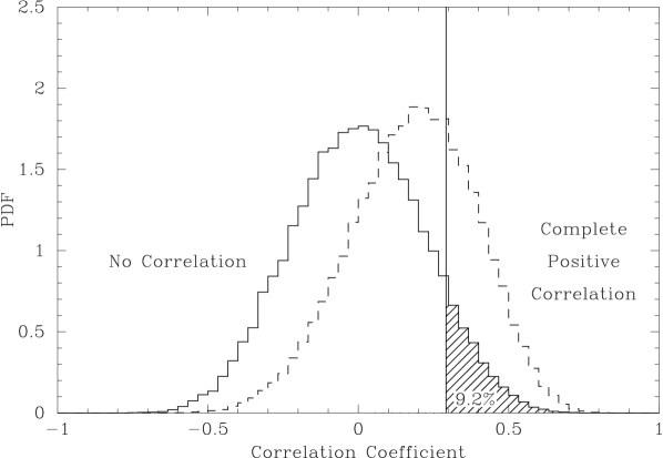
Figure 2: Probability distribution functions (PDF) of linear correlation coefficient for simulated data sets. The solid curve shows the distribution obtained for uncorrelated simulated data. The dashed curve shows the distribution obtained for simulated data with a complete positive correlation between magnifications and residuals. The value of the linear correlation coefficient obtained for the data ($r=0.29$) is indicated by the vertical solid line. The probability of obtaining a correlation coefficient higher than this value in the case of no correlation is $9.2\%$.

References

- [1] Holz D and Linder E 2005 Astrophys. J. 631 678
- [2] Williams L L R and Song J 2004 Mon. Not. R. Astron. Soc. 351 1387
- [3] Ménard B and Dalal N 2005 Mon. Not. R. Astron. Soc. 358 101
- [4] Capak P, et al2004 Astron. J. 107 180
- [5] Giavalisco M, et al2004 Astrophys. J. 600 L93
- [6] Strolger L, et al2004 Astrophys. J. 613 200
- [7] Riess A, et al2004 Astrophys. J. 607 665
- [8] Riess A, et al2007 To appear in Astrophys. J [astro-ph/0611572]
- [9] Jönsson J, Dahlén T, Goobar A, Gunnarsson C, Mörtsell E, and Lee K 2006 Astrophys. J. 639 991
- [10] Gunnarsson C 2004 J. Cosmol. Astropart. Phys. 0403 002
- [11] Navarro J F, Frenk C S and White S D M 1997 Astrophys. J. 490 93
- [12] Gunnarson C, Dahlén T, Goobar A, Jönsson J, and Mörtsell E 2006 Astrophys. J. 640 417