The Shape of the Gravitational Potential in Cold Dark Matter Halos

Abstract

We use a set of cosmological N-body simulations to investigate the structural shape of galaxy-sized cold dark matter (CDM) halos. Unlike most previous work on the subject—which dealt with shapes as measured by the inertia tensor—we focus here on the shape of the gravitational potential, a quantity more directly relevant to comparison with observational probes. A further advantage is that the potential is less sensitive to the effects of substructure and, as a consequence, the isopotential surfaces are typically smooth and well approximated by concentric ellipsoids. Our main result is that the asphericity of the potential increases rapidly towards the centre of the halo. The radial trend is more pronounced than expected from constant flattening in the mass distribution, and reflects a strong tendency for dark matter halos to become increasingly aspherical inwards. Near the centre the halo potential is approximately prolate on average ($(c/a)_{0}=0.72\pm 0.04$, $(b/a)_{0}=0.78\pm 0.08$), but it becomes less axisymmetric and more spherical in the outer regions. The principal axes of the isopotential surfaces remain well aligned, and in most halos the angular momentum tends to be parallel to the minor axis and perpendicular to the major axis. This suggests that galactic disks may form in a plane where the potential is elliptical and where its ellipticity varies rapidly with radius. This can result in significant deviations from circular motion in systems such as low surface brightness galaxies (LSBs), even for relatively minor deviations from circular symmetry. Simulated long-slit rotation curves often appear similar to those of LSBs cited as evidence for constant density “cores”. This suggests that taking into account the 3D shape of the dark mass distribution might help to reconcile such evidence with the cuspy mass profile of CDM halos.

1 Introduction

The flat rotation curves of disk galaxies (Rubin & Ford, 1970; Roberts & Whitehurst, 1975), together with the anomalously high velocity dispersion of galaxies in clusters (Zwicky, 1933), constituted the first compelling evidence for the existence of a massive dark matter component in the Universe. Since the interpretation of these data depends on the structure of dark matter halos, many theoretical studies have focused on the radial distribution of mass within virialized dark matter halos, both analytically (Gunn & Gott, 1972; Fillmore & Goldreich, 1984; Hoffman & Shaham, 1985) and numerically (Frenk et al., 1985, 1988; Quinn et al., 1986; Dubinski & Carlberg, 1991; Crone et al., 1994). This effort culminated in the realization that, in the prevailing cold dark matter (CDM) paradigm, the spherically averaged mass profile of dark halos is accurately described by scaling an approximately “universal” profile (Navarro et al., 1996, 1997, NFW). The fitting formula proposed by NFW has enabled a simple means of testing the theoretical expectations against observations. Overall, these studies have shown that the mass profile of cold dark matter halos is broadly consistent with observations of X-ray clusters, gravitational lensing, satellite dynamics, and galaxy group properties (Pointecouteau et al., 2005; Comerford et al., 2006; Prada et al., 2003; Mandelbaum et al., 2006), although problems remain, especially on the scale of galaxies.

A particularly contentious debate has centred on the inner slope of the density profile inferred from rotation curves of low surface brightness (LSB) disk galaxies. Many authors have argued for the presence of a constant density ‘core’ at the centre of galactic dark matter halos, in direct contradiction with the ‘cuspy’, centrally divergent density profile of simulated CDM halos (see, e.g., Flores & Primack, 1994; Moore, 1994; McGaugh & de Blok, 1998; de Blok et al., 2001). This conclusion relies on the assumption that the disk is in circular motion and, therefore, that the observed rotation velocity is a fair tracer of the circular velocity of the halo. This assumption holds only for thin, cold, gaseous disks in spherically symmetric potentials and, while this is a convenient assumption for preliminary studies, it has long been known that CDM halos are not spherically symmetric objects (Frenk et al., 1988; Dubinski & Carlberg, 1991; Warren et al., 1992; Thomas et al., 1998; Jing & Suto, 2002; Bailin & Steinmetz, 2005; Bett et al., 2006).

Recently, Hayashi & Navarro (2006, hereafter HN) investigated the kinematics of a gaseous disk in a triaxial halo potential using analytic solutions for closed loop orbits. The shape of the disk rotation curve, as measured by a long-slit spectrum, depends on the orientation of the slit, the inclination of the disk, and the radial dependence of the departures from spherical symmetry. HN show that significant deviations from circular motion may result even in very mildly triaxial potentials, since the orbital shape is controlled by the ratio of escape to circular velocities, a quantity that increases steadily inwards in CDM halos.

Few signatures of the halo triaxial structure—which may be recognised in 2D velocity fields—are discernible in long-slit observations. Linearly-rising “core-like’ rotation curves may occur if (i) the slit samples velocities near the long axis of the (elliptical) closed orbits and if (ii) the deviations from spherical symmetry in the halo potential become more pronounced towards the centre. As noted above, the shapes of CDM halos have been studied previously; however, these studies have focused on inertia-tensor shapes rather than on the potential, thus it is still unclear whether the radial dependence of halo triaxiality is quantitatively consistent with the latter requirement.

Establishing the typical radial dependence of triaxiality in the potential of CDM halos is therefore one of the main concerns of this paper. The interest of this study goes beyond the topic of LSB rotation curves, since the non-spherical nature of CDM halos affects the interpretation of a variety of observational probes, including the kinematics of polar ring galaxies (Sackett et al., 1994), the warping and flaring of galactic disks (Teuben, 1991; Olling & Merrifield, 2000), and the morphology of tidal streams. In a spherical potential, tidal streams remain confined to a plane, whereas the plane of motion will precess gradually in non-spherical halos. Ibata et al. (2001) use this to interpret tidal debris from the Sagittarius dwarf galaxy, and conclude that the halo of the Milky Way is spherical and therefore possibly in conflict with CDM predictions. However, Helmi (2004) argues that the Sagittarius stream may be too dynamically young to be sensitive to the shape of the dark matter halo, and hence may be consistent with a Milky Way halo as triaxial as a typical simulated CDM halo (see also Law et al., 2005; Johnston et al., 2005).

In galaxy clusters, the hot intracluster gas is in equilibrium with the gravitational potential of the cluster, and the isodensity surfaces of the gas coincide with the isopotential surfaces of the cluster halo (BUOTE94; BUOTE02; LEE03; FLORES05). Observations of X-ray emission and Sunyaev-Zel’dovich (S-Z) decrement measure the integrated density along the line-of-sight though the cluster, therefore the shape of the X-ray isophotes and S-Z contours reflects the shape and orientation of the underlying dark matter halo potential. Models of the projected surface brightness profiles as a function of cluster orientation and triaxiality have been developed by LEE04 and WANG04, but these are based on a constant triaxiality in the gas isodensity surfaces, which may not be an accurate representation of the distribution of gas in equilibrium with a realistic CDM halo potential

There is therefore considerable interest in firming up the theoretical expectation for the shape and radial dependence of the gravitational potential in CDM halos, and this paper aims to provide guidance for such modelling. We focus here on the shape of the isopotential surfaces of galaxy-sized dark matter halos using high-resolution cosmological N-body simulations.

The outline of the paper is as follows. In Section 2 we describe the simulations and methods we use to calculate halo shapes. In Section 3 we present our measurements of the shapes of halos and of the internal alignment of halo shapes. In Section 4 we investigate the flattening of the mass distribution required to reproduce the radial dependence of the halo potential shapes, and we present a simple fitting formula to approximate the potential of a triaxial CDM halo. Finally, we apply this result in Section 5 to the kinematics of disks in realistic triaxial CDM halo potentials. We conclude with a brief summary in Section 6.

2 Simulations and Methods

This study is based on a suite of cosmological N-body simulations of seven Milky Way-sized galaxy halos and four dwarf galaxy-sized halos. The concordance $\Lambda$CDM cosmology is adopted for these simulations, with $\Omega_{0}=0.3$, $\Omega_{\Lambda}=0.7$, $\sigma_{8}=0.9$. and either $h=0.65$ (runs labelled G1, G2 and G3) or $h=0.7$ (the rest). These simulations make use of the techniques described in detail in Power et al. (2003) and Navarro et al. (2004) for resimulating halos at high resolution using nested regions of particles with different mass resolution and gravitational softening lengths in order to maximize the number of particles which end up in the target halo at $z=0$.

Each halo contains about $N\simeq 10^{6}$ particles within the virial radius, $r_{200}$, defined as the radius of a sphere of mean density equal to $200$ times the critical density for closure. The spherically-averaged mass profile of these halos is robust down to $r_{\rm conv}\simeq 0.01~{}r_{200}$ according to the convergence criteria described in Power et al. (2003). Table LABEL:tab:halos summaries the main properties of the simulated halos; a full description of the numerical details of these simulations and an analysis of the halo mass profiles is presented in Hayashi et al. (2004) and Navarro et al. (2004).

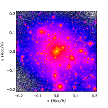
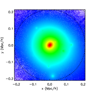
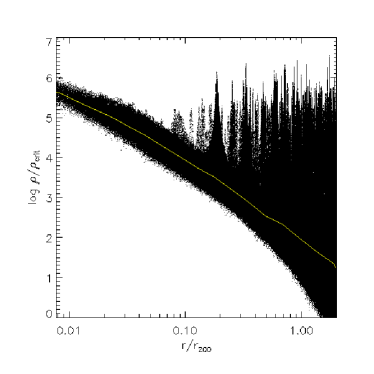
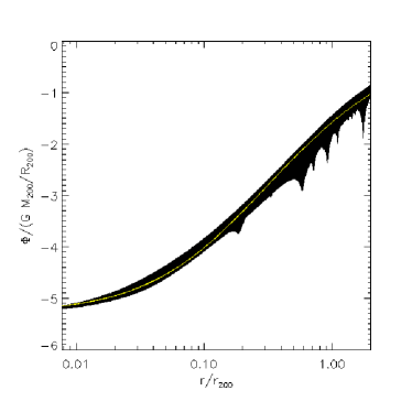
Figure 1: Upper panels: Halo G3/$256^{3}$ coloured by local density (left) and potential (right). Color scheme is logarithmic for density and linear for the potential. The virial radius, $r_{200}$, is shown by the dashed circle. Lower panels: Local density (left) and potential (right) of particles as a function of radius. Thin solid lines show the average local density (left panel) and best fit NFW potential (right panel).

Figure 1 shows one galaxy-sized halo from our set of simulations. The upper panels show the halo with its particles coloured according to the values of their local density (left) and gravitational potential (right). The local density of each particle is computed by averaging over its 64 nearest neighbour particles with a spline kernel similar to that used in Smoothed Particle Hydrodynamics (SPH) calculations. The gravitational potential of each particle is computed using all particles within $4~{}r_{200}$ of the halo centre, determined using an iterative technique in which the centre of mass of particles within a shrinking sphere is computed recursively until a few thousand particles are left (Power et al., 2003). The bottom panels plot the values of the density and gravitational potential of each particle as a function of its distance from the halo centre.

The most striking feature of this figure is that the wealth of halo substructure readily apparent in local density, is much less prevalent in the gravitational potential. This is not only because the potential is an integral (and therefore more uniform) quantity, but also because the total amount of mass associated with substructure is typically only $5-10\%$ of the mass within $r_{200}$ (see, e.g., De Lucia et al., 2004). The lower left panel of Figure 1 shows that particles within substructures (subhalos) appear as sharply defined “spikes” which can exceed the mean local density at the radius of the subhalo by many orders of magnitude. This can cause undesirable biases when measuring halo shapes. For instance, Jing & Suto (2002) estimate shapes using isodensity surfaces, a procedure that requires a careful, and somewhat arbitrary, removal of substructure as a preliminary step, and that may thus introduce ambiguities in the results.

In comparison, as emphasised by Springel et al. (2004), the isopotential surfaces are much smoother and relatively insensitive to the presence of substructure. The lower right panel of Figure 1 shows that the gravitational potential of particles in subhalos deviates from the mean value at the subhalo radius by at most a factor of two. Furthermore, it is the gravitational potential and not the local density that is the more relevant quantity in most dynamical studies of halo structure.

In order to measure the three-dimensional shape of a halo’s isopotential surfaces, we adopt the method described by Springel et al. (2004). The gravitational potential is first computed on three uniform grids covering orthogonal planes which intersect at the location of the minimum gravitational potential of the halo. In our standard set-up, these meshes have $1024^{2}$ cells and extend to a distance of $2~{}r_{200}$. We use a hierarchical tree algorithm to compute the potential efficiently and include all the mass out to a radius of $4~{}r_{200}$ when processing an individual halo, while more distant particles are ignored.

If the isopotential surfaces are ellipsoids, then their intersections with the three principal planes are ellipses, and the full shape information of each ellipsoid can be recovered uniquely from the shapes of the intersections. Compared to a full 3D grid, using just three planes has the important advantage of allowing a much finer mesh while reducing the memory and computational requirements by several orders of magnitudes.

In our actual fitting procedure, we first determine in each plane the intersections of 360 radial rays with constant angular separation with the isopotential ellipses for a chosen value of the potential. We define the potential at every point in the planes by bi-linear interpolation in the corresponding two-dimensional grid. We adopt the centre-of-mass of the resulting set of points as the centre of the isopotential ellipsoid, and identify its principal axes with the eigenvectors of the moment-of-inertia tensor of the sample of points. To determine the axis lengths $(a,b,c)$ , we first express the coordinates of the points in the orthonormal basis of the principal axis relative to the ellipsoid’s centre. Denoting these coordinates with $(x_{i},y_{i},z_{i})$ we then define a normalized radius $r_{i}$ for each point as

$$\frac{x_{i}^{2}+y_{i}^{2}+z_{i}^{2}}{r_{i}^{2}}=\frac{x_{i}^{2}}{a^{2}}+\frac{y_{i}^{2}}{b^{2}}+\frac{z_{i}^{2}}{c^{2}}.$$ (1)

If a point lies on the ellipsoid, $r_{i}$ would just equal the Cartesian distance $\sqrt{x_{i}^{2}+y_{i}^{2}+z_{i}^{2}}$, and the left-hand-side of equation (1) would be unity. To determine the best-fitting axis lengths, we therefore minimize the quantity

$$S=\sum_{i}\left(r_{i}-\sqrt{x_{i}^{2}+y_{i}^{2}+z_{i}^{2}}\right)^{2}$$ (2)

with respect to $(a,b,c)$. In practice, we use a Newton-Raphson method to alternatingly find the roots in $\frac{\partial S}{\partial a}=0$, $\frac{\partial S}{\partial b}=0$, and $\frac{\partial S}{\partial c}=0$, cycling through the equations until no further reduction of $S$ can be achieved.

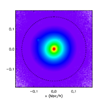
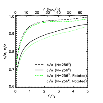
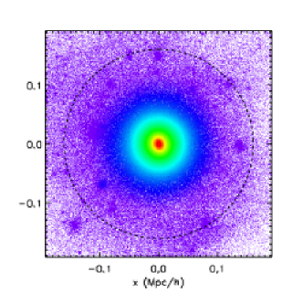
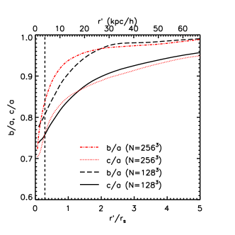
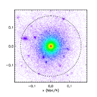
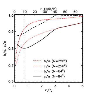
Figure 2: Halo G7 simulated at three different resolutions. The number of particles varies by a factor of 8 between each realization. Left panels: Halo particles coloured by gravitational potential. Right panels: Axial ratios $b/a$ and $c/a$ measured by fitting ellipsoids to isopotential contours on three orthogonal planes through the halo as a function of the elliptical radius $r^{\prime}=(a^{2}+b^{2}+c^{2})^{1/2}$. The vertical dashed line shows the minimum converged radius in the mass profile, $r_{\rm conv}$, in each simulated halo. The top right panel shows the axial ratios calculated using two sets of orthogonal planes rotated by an arbitrary angle. The axial ratios measured in both cases are in good agreement and differ by $\mathrel{\hbox{\hbox to0.0pt{\hbox{\lower 4.0pt\hbox{$\sim$}}\hss}\hbox{$<$}}}~{}3\%$ at all radii.

Figure 2 shows the results of this procedure applied to galaxy halo G7. The right panels show the ratio of the semimajor axes of the best fitting ellipsoids, $b/a$ and $c/a$, where $c<b<a$, as a function of the radius $r^{\prime}=\sqrt{a^{2}+b^{2}+c^{2}}$. The radius is plotted in units of the NFW scale radius, $r_{s}$ (where the logarithmic slope of the density profile is equal to the isothermal value of $-2$), determined by fitting the spherically-averaged density profile with the NFW fitting formula.

The top panels show the highest resolution realization, G7/256³, which has $N_{200}\simeq 3.5\times 10^{6}$ particles within $r_{200}$ (shown by a circle in the left panels). Both the minor-to-major ($c/a$) and intermediate-to-major ($b/a$) axial ratios decrease gradually inwards, with evidence of a sharp decrease inside the scale radius. The top right panel also illustrates the uncertainty in the shape measurements by plotting the axial ratios calculated using two sets of orthogonal planes rotated by an arbitrary angle. The axial ratios measured in both cases are in good agreement and differ by $\mathrel{\hbox{\hbox to0.0pt{\hbox{\lower 4.0pt\hbox{$\sim$}}\hss}\hbox{$<$}}}~{}3\%$ at all radii, confirming the applicability of approximating the isopotential surfaces as ellipsoids.

The middle and lower panels of Figure 2 show the results for two lower resolution simulations of the same halo G7. The realizations labelled $N=128^{3}$ and $N=64^{3}$ have $N_{200}\simeq 3.3\times 10^{5}$ and $4.2\times 10^{4}$, respectively. The axial ratios of G7/$128^{3}$ are in good agreement with those of the high resolution $N=256^{3}$ run, with maximum deviations of $\simeq 4\%$. In the lowest resolution run, however, although the general trend in the axial ratios is reproduced, large deviations are apparent at small radii. Near the centre, G7/64³ is significantly more spherical than higher resolution realizations, suggesting that the steep inward increase in asphericity seen in G7/128³ and G7/256³ is a result of the inner structure of the halo, which is poorly resolved in the case of G7/64³. The two-body relaxation timescale depends on the number of particles and the gravitational softening length and therefore is shortest near the centre. This may result in a more spherical distribution of particles, which in turn can cause the potential to be more spherical near the centre of low resolution halos. We investigate this possibility in Section 4, but for the rest of the analysis we use only simulations of resolution comparable to the 256³ realization of halo G7.

3 Halo Shapes and Internal Alignment

3.1 Radial dependence of isopotential shapes

Because the monopole dominates in the outer regions of a centrally concentrated mass distribution, the isopotential surfaces are expected to become more spherical in the outer regions. The precise radial variation of the shape depends on the distribution of mass within the halo and on the radial dependence of its flattening.

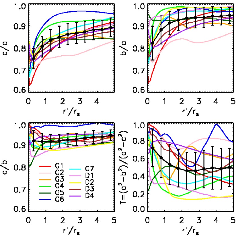
Figure 3: Isopotential shapes of all halos as a function of radius, where $c$, $b$, and $a$, are the lengths of the minor, intermediate and major axes, respectively, and the radius is given in units of the NFW scale radius of the density profile, $r_{s}$. The triaxiality parameter $T=(a^{2}-b^{2})/(a^{2}-c^{2})$ is equal to 0 (1) for a perfectly oblate (prolate) spheroid. Points with error bars show the mean $\pm 1~{}\sigma$ of all axial ratio profiles. Halos clearly tend to become more aspherical towards the centre, a gradual trend that becomes increasingly steep inside $r_{s}$. On average, halos are very nearly prolate at the centre, but become more spherical and less axisymmetric in the outer regions.

Figure 3 shows the axial ratio profiles for all of the simulated halos in our sample along with the average profile (computed after scaling each profile to its scale radius, $r_{s}$) with 1$\sigma$ error bars to indicate the scatter. The slow approach to spherical symmetry in the outer regions is clear in all cases (the average minor-to major axial ratio at $r=5~{}r_{s}$ is $c/a\simeq 0.9$), as is the sharp inward increase in asphericity inside the scale radius. Near the centre, $c/a$ and $b/a$ approach similar values, $0.72$ and $0.78$, respectively, but the system becomes more spherical and less axisymmetric in the outer regions. Figure 3 also shows the triaxiality parameter, defined as $T=(a^{2}-b^{2})/(a^{2}-c^{2})$, where $T=0~{}(1)$ for a perfectly oblate (prolate) spheroid. On average, $T>0.5$ for $r<r_{s}$ indicating that halos tend toward prolate shapes near the centre. The $c/b$ profiles remain relatively flat from the centre outwards, increasing from a central value of $\sim 0.92$ to $\sim 0.94$ in the outer parts of the halo.

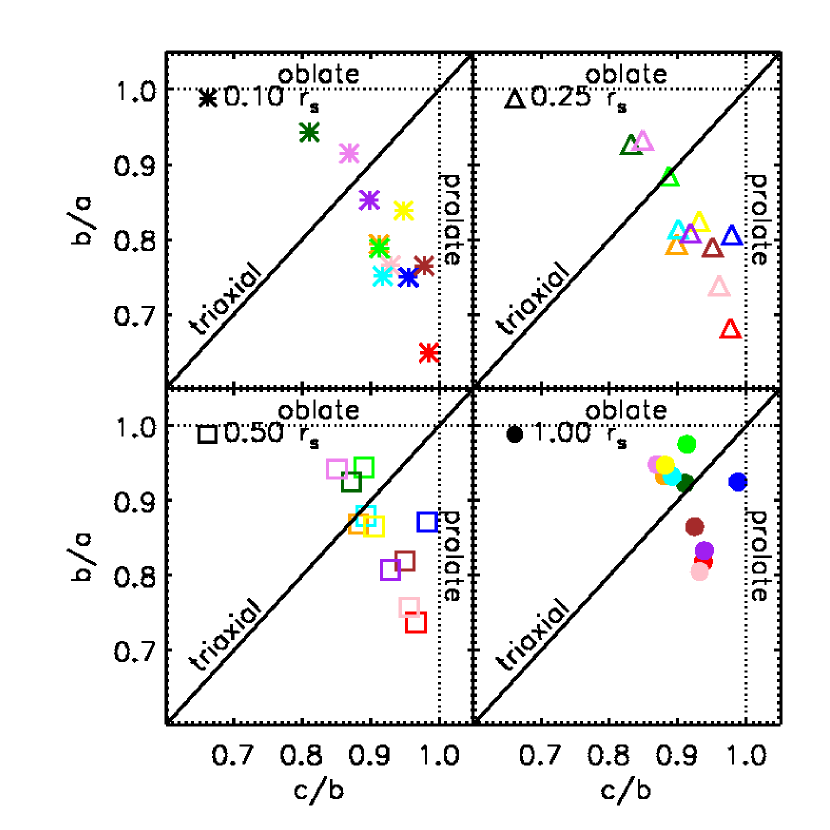
Figure 4: Intermediate-to-major ($b/a$) versus minor-to-intermediate $(c/b)$ axial ratios at four different radii within $r_{s}$. Perfectly oblate (prolate) halos have $b/a=1$ ($c/b=1$) and “maximally triaxial” halos have $b/a=c/b$. Halos tend to become more prolate inwards.

A more detailed view of this inner region is shown in Figure 4, where we plot $b/a$ versus $c/b$ at four different radii, $r=0.1,0.25,0.5$, and $1.0~{}r_{s}$. Note that a perfectly oblate spheroid corresponds to $b/a=1$, whereas a prolate spheroid corresponds to $c/b=1$. There is a clear trend for halos to become increasingly prolate near the centre. At $r=r_{s}$, five out of eleven halos are more prolate than oblate, but at $r=0.1~{}r_{s}$, all but two of the halos are more prolate than oblate.

The significant variation in the shape of the halo potential with radius may complicate detailed comparisons of the shapes of simulated halos with those inferred from X-ray and S-Z observations. In the model of LEE04, for example, this variation is neglected in order to simplify the calculation of the projected surface brightness profile of a galaxy cluster. The large range in axial ratio values at $r\mathrel{\hbox{\hbox to0.0pt{\hbox{\lower 4.0pt\hbox{$\sim$}}\hss}\hbox{$<$}}}2~{}r_{s}$ suggests that comparing axial ratios measured at large radii might be a more straightforward test of the distribution of shapes. Observing an increase in the ellipticity of X-ray isophotes or S-Z isodecrement contours towards the centre in individual cluster systems would also provide strong evidence for the existence of an underlying CDM halo potential.

3.2 Alignments

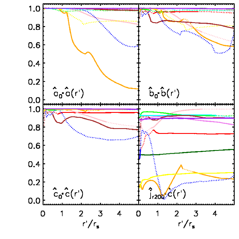
Figure 5: Alignment of principal axes as a function of radius. Vector $\hat{a}(r^{\prime})$ represents the unit vector along the major axis of the halo, and $\hat{a}_{0}=\hat{a}(r^{\prime}\simeq r_{\rm conv})$. Dotted lines indicate radii where $c/b>0.95$ and/or $b/a>0.95$. For these nearly axisymmetric systems two of the axes’ directions are poorly determined. In eight of the eleven halos, the principal axes are well aligned with radius throughout the main body of the halo. In most halos $\hat{j}_{r200}\cdot\hat{c}(r)\simeq 0.9$, indicating alignment of $25^{\circ}$ or better between the minor axis and the angular momentum vector of the halo.

The alignment of the isopotential surfaces as a function of radius is illustrated in Figure 5, which shows the cosine of the angle between the principal axes of the isopotential at the “converged” radius and the corresponding axis at larger radii. Since orientations between some axes will be poorly determined in cases where $b\simeq a$ or $c\simeq b$, we plot the results using solid (dotted) curves in Figure 5 when the length of the axis plotted differs by more (less) than $5\%$ from the lengths of the other axes. Taking this into account, we find that in most cases where the axes are well determined the isopotential surfaces appear to be reasonably well aligned as a function of radius, with the possible exception of halos G2, G3, and D3.

The bottom-right panel of Figure 5 also shows the relative alignment between the potential and the angular momentum of the halo, by plotting the cosine of the angle between the minor axis and the total angular momentum, computed using all particles within $r_{200}$. We find that the minor axis tends to be aligned with the angular momentum vector in most halos; in six of the eleven halos, the alignment between the minor axis and the angular momentum vector is better than $25^{\circ}$ out to $\simeq 5~{}r_{s}$.

The latter result has important implications for the dynamics of disk galaxies since baryons and dark matter are expected to have acquired similar (specific) angular momenta, and, therefore, the rotation axis of a galactic disk would be aligned with the halo’s net angular momentum (see, e.g., Fall & Efstathiou, 1980; van den Bosch et al., 2002; Navarro et al., 2004; Abadi et al., 2006). Such a disk would be confined to a plane containing the major and intermediate axes of the halo. In a nearly prolate halo the potential in such plane would deviate significantly from circular symmetry.

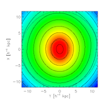
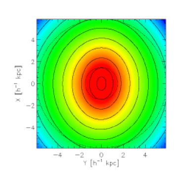
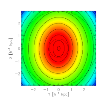
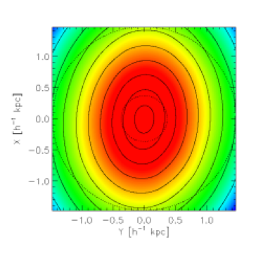
Figure 6: Gravitational potential of halo D3 on the plane perpendicular to its minor axis, corresponding to the plane in which a disk might form. The radii of the outer dotted circles are $4,2,1,$ and $0.5~{}r_{s}$ in the top left, top right, bottom right panels, respectively, where $r_{s}=2.94~{}\>h^{-1}{\rm kpc}$. The radius of the inner circles is $0.25\times$ that of the outer circle. The ellipticity of the isopotential contours (solid curves) clearly increases towards the centre of the halo.

We show this explicitly in Figure 6 where we plot the potential of halo D3 on the plane containing its major and intermediate axes. The isopotential contours are clearly noncircular but are well-approximated by ellipses. The four panels in Figure 6 show the halo on increasingly small scales in order to highlight the increase in the ellipticity of the isopotential contours towards the centre of the halo. We investigate the consequences of this for the dynamics of a gaseous disk in Section 5.

4 A Simple Model for Halo Triaxiality

The radial dependence of the shape of the potential is dictated by both the flattening and the mass profile of the halo. Here we explore the effects of each in order to shed light on the steep radial dependence of the halo asphericity discussed in the previous section.

To this aim, we generate a spherically symmetric NFW halo model with $N=10^{6}$ particles out to a maximum radius of $10~{}r_{s}$. We set the gravitational softening length to $0.05~{}r_{s}$. We turn this into a prolate halo of constant flattening by multiplying the x- and y-coordinates of all particles by a factor of $0.4$. We then use the ellipsoid fitting method described in the previous section to measure the shapes of the isopotential surfaces as a function of radius. We also measure the shape of the mass distribution by diagonalizing the inertia tensor according to the iterative procedure of Katz (1991). This method measures the shape using all particles within an ellipsoid whose volume is approximately equal to the volume of a sphere of radius $r$.

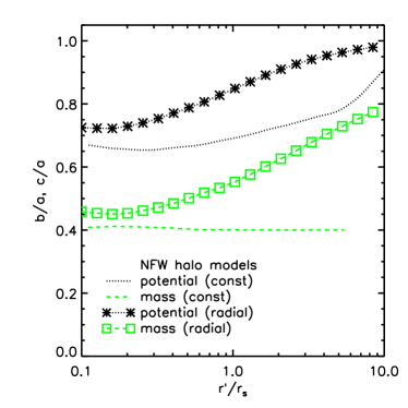
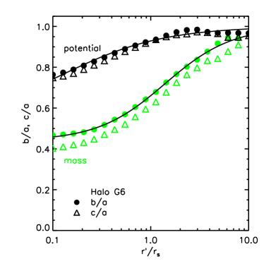
Figure 7: Left panel: Axial ratios of NFW halo models with constant (lines without symbols) and radially varying (symbols) flattening in the mass distribution as a function of radius. Right panel: Axial ratios of halo G6 as a function or radius. Solid curves show fits to the axis ratio profiles with eq. (3). Halo models with constant flattening cannot reproduce the axial ratio profiles of simulated halos like G6, which require increasing asphericity towards the centre.

Figure 7 compares the shape of the self-similar prolate NFW halo (left panel) and halo G6 (right panel). The dashed curve (without symbols) in the left panel shows the axial ratio measured using the inertia tensor; as expected, a constant value of $\approx 0.4$ is recovered for the prolate NFW model. The potential axial ratio (dotted curve without symbols) is not constant, but the radial dependence is much gentler than seen in halo G6. Within $r_{s}$ the shape of the potential of the prolate NFW model remains more or less constant at $\sim 0.65$; and becomes gradually more spherical outside $r_{s}$. This differs from the radial behaviour of the axial ratios in halo G6 (right panel) where both the potential and inertia shapes within $r_{s}$ increase from the centre outwards. These results indicate that the sharp increase in the asphericity of the halo potential is inconsistent with a constant flattening in the mass distribution and reflects the presence of a radially varying distortion in the mass distribution as well.

A convenient approximation of the shape profiles is provided by the following formula:

$$\log\left({b\over a}\ {\rm or}\ {c\over a}\right)=\alpha\left[\tanh\left(\gamma\log\frac{r}{r_{\alpha}}\right)-1\right].$$ (3)

Here $\alpha$ parameterizes the central value of the ratio, such that $(b/a)_{0}$ or $(c/a)_{0}$ is given by $10^{-2~{}\alpha}$, $r_{\alpha}$ indicates the characteristic radius at which the axial ratio rises a significant amount from its central value, and $\gamma$ regulates the sharpness of the transition. This fitting formula gives a reasonably accurate description of the axial ratio profiles of both the mass distribution and the isopotential surfaces in the simulations, as shown by the fits to the G6 shape profiles in Figure 7 (lines through symbols in its right panel). The best fit parameter values for fits to the mass and isopotential shapes are given in Table LABEL:tab:halos.

An NFW halo model with a radially varying flattening is a much better approximation to the radial behaviour of the shapes seen in the simulations. This is shown in the left panel of Figure 7, where the same (initially spherical) NFW model is modified by multiplying the x- and y- coordinates of particles at radius $r$ by eq. (3) evaluated with ($\alpha,r_{\alpha},\gamma$) = $(0.2,1.0~{}r_{s},1.3)$. This choice is motivated by the best fit to the $b/a$ profile of the mass distribution of halo G6.

The axial ratio profiles of the resulting halo model are shown by the symbols in the left panel of Figure 7. The distortion in the shape of the isopotential surfaces of this halo is clearly reminiscent of that of halo G6. The agreement is not exact, however, because the inertia tensor measures the shape using all particles within a given volume and therefore does not correspond to a transformation applied to the coordinates of particles as a function of radius. However, the model does demonstrate that a distortion in the mass distribution which increases towards the centre of the halo can reproduce the radial variation observed in the isopotential shapes of halos like G6.

We also find that in all cases, the potential axial ratio profile becomes flat, or increases slightly, toward the centre of the halo. In G6 and the radially varying NFW model, this coincides with a similar trend in the mass axial ratio profile. However, in the NFW model with a constant flatenning, the shape of the potential becomes more spherical near the centre, but the shape of the mass distribution remains constant at all radii. This suggests that the finite gravitational softening length may be responsible for making the potential more spherical near the centre, although two-body relaxataion effects may also play a role near the centres of simulated halos like G6 and the low resolution versions of G7 shown in Figure 2.

We note that the ratio of the potential axial ratio to the mass axial ratio varies as a function of radius for both the constant and radially varying flatenning models. In terms of the eccentricity parameter used in the models of LEE03 and LEE04, $e=\sqrt{1-(b/a)^{2})}$, the ratio of potential eccentricity to the mass eccentricity varies from $\sim 0.8$ to $\sim 0.6$, and $\sim 0.8$ to $\sim 0.3$, in the constant and radially varying cases, respectively. In comparison, the eccentricity ratio of the LEE03 model varies from $0.77$ to $0.4$, however, LEE04 approximate this with a constant value of $0.49$ in order to calculate the projected surface brightness distribution of their model. Since this ratio varies over roughly the same range for the model with a radially varying flatenning, we conclude that the assumption of a constant ratio is no worse in this case than it is for models with constant flatenning.

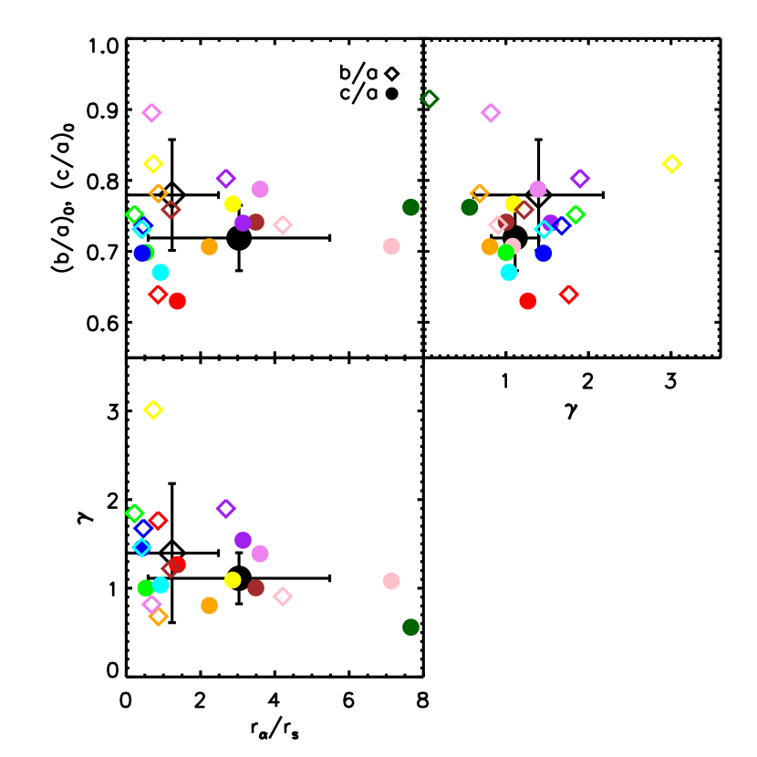
Figure 8: Values of central axial ratios, $(b/a)_{0}$ and $(c/a)_{0}$, and parameters $r_{\alpha}$ and $\gamma$ obtained by fitting eq. (3) to the $b/a$ and $c/a$ axial ratio profiles plotted in Figure 3. Large symbols with error bars show the average and standard deviation for all halos. The average transition scale for the $c/a$ profiles is about twice that of the $b/a$ profiles, indicating that the former tend to increase more gradually than the latter profiles

The best fit parameters using eq. (3) to approximate the potential axial ratio profiles of all our simulated halos are listed in in Table LABEL:tab:halos and shown in Figure 8. Although there is substantial halo-to-halo scatter, several trends are apparent. The large symbols with “error bars” in Figure 8 show the average value of each parameter and the 1-sigma scatter. The central axial ratios scatter about $(b/a)_{0}=0.78\pm 0.08$ and $(c/a)_{0}=0.72\pm 0.04$. The average transition radius, expressed in units of the scale radius, $r_{\alpha}/r_{s}$, is $1.2\pm 1.2$ for the $b/a$ profiles (excluding halo G5 which has an almost flat $b/a$ profile, and therefore an extremely large and poorly defined value of $r_{\alpha}$) and $3.0\pm 2.4$ for the $c/a$ profiles. The average value of $\gamma$ is $1.4\pm 0.8$ for the $b/a$ profiles and $1.1\pm 0.3$ for the $c/a$ profiles. On average, $c/a$ profiles tend to increase more gradually than $b/a$ profiles, and profiles become more spherical and less axisymmetric at larger radii.

Our results may be used to construct a model for the gravitational potential of a triaxial CDM halo by using eq. (3) to modify the potential of a spherical NFW model.

$$\Phi(x,y,z) = \Phi_{\rm NFW}(r^{t})$$ (4)

$$r^{t} = r\sqrt{\left(\frac{x}{a(r)}\right)^{2}+\left(\frac{y}{b(r)}\right)^{2}+\left(\frac{z}{c(r)}\right)^{2}}$$ (5)

$$\Phi_{\rm NFW}(r) = -\frac{GM_{200}}{r_{s}f(c_{200})}\frac{\ln(1+r/r_{s})}{r/r_{s}},$$ (6)

where the concentration parameter $c_{200}=r_{200}/r_{s}$ and $f(u)=\ln(1+u)-u/(1+u)$. Since eq. (3) describes only the ratios between the lengths of the principal axes, the normalisation is set by assuming that at each radius $r$, the volume of the ellipsoid with semi-axis lengths $a(r),b(r)$ and $c(r)$ is equal to $4\pi r^{3}/3$, i.e., $a(r)b(r)c(r)={r^{3}}$, which implies

$$a(r)=r\ (b/a)^{-1/3}(c/a)^{-1/3},$$ (7)

where $b/a$ and $c/a$ are functions of $r$ given by eq 3. This ensures that the spherically-averaged potential of the triaxial model will be similar to that of a spherically symmetric NFW model with the same mass and scale radius.

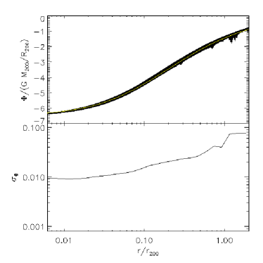
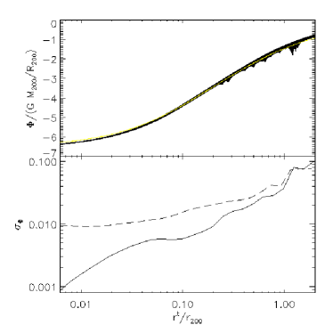
Figure 9: Left panels: Potential versus radius of particles in halo G5. The solid line shows the profile of a best fit NFW potential. The lower panel shows the residuals from the fit, $\sigma_{\Phi}$ as a function of radius. Right panel: Same as left but plotted versus the reduced radius $r^{t}$ of the best fitting ellipsoid (see eq. 5). The dashed line in the lower panel indicates the same residuals, $\sigma_{\Phi}$, as in the left panel. The residuals are significantly reduced at small radii where substructure does not dominate the scatter.

We show that this model provides a good description of the potential of simulated halos in Figure 9 where we compare the gravitational potential of particles in halo G5 plotted against their radius, $r$, and against the reduced radius, $r^{t}$, given by eq. (5). The reduced radius is calculated by rotating the halo so that its principal axes are aligned with the x-, y-, and z-coordinate axes. The bottom panels of this figure show that the dispersion in the potential profile is significantly reduced when expressed in terms of the reduced radius; in the inner regions, $r\mathrel{\hbox{\hbox to0.0pt{\hbox{\lower 4.0pt\hbox{$\sim$}}\hss}\hbox{$<$}}}2~{}r_{s}$, the dispersion is reduced by a factor of two. At larger radii, the presence of substructure dominates the scatter in the potential and the triaxial modelling has less impact.

We conclude that taking into account halo triaxiality provides a substantial improvement over spherically symmetric CDM halo models. The fitting formula given by eq. (3) along with parameter values in the ranges we find for simulated halos, listed in Table LABEL:tab:halos, provides a simple analytic model for a realistic, triaxial CDM halo potential. This model may be of practical use for N-body simulations of tidal streams like those of Ibata et al. (2001) and Helmi (2004), and in calculations of the X-ray and S-Z surface brightness distributions of triaxial galaxy clusters as in LEE04.

5 Disk Kinematics in Triaxial CDM Halos

We explore now the kinematics of disks in CDM halos with radially varying triaxiality. We assume that the disk lies in one of the principal planes of the potential, and therefore the problem is reduced to two dimensions. Our approach follows closely the formalism presented in HN, where analytic closed loop orbit solutions are found to describe the orbits in a thin, filled, gaseous disk. These solutions use the epicyclic approximation to find closed orbits in a potential of the form:

$$\Phi(R,\phi)=\Phi_{0}(R)+\Phi_{m}(R)\cos(m\phi_{0})$$ (8)

where $\Phi_{0}(R)$ is the unperturbed (circularly-symmetric) potential, $\Phi_{m}(R)$ is a stationary perturbation to that potential, and $\phi$ is the azimuthal angle. For $m=2$ and small perturbations, the perturbation is periodic in $180^{\circ}$ and the isopotential contours are roughly elliptical in shape. The closed loop orbits solutions are also roughly elliptical, but are oriented with their major axes perpendicular to those of the isopotential contours.

The tangential velocity along the orbit oscillates about the circular velocity of the unperturbed potential, $V_{c}(R)=({R\,{\rm d}\Phi_{0}/{\rm d}R})^{1/2}$, and the deviations from $V_{c}$ will be maximal at pericentre and apocentre of the orbit. Long-slits aligned with these directions would yield rotation curves whose shape will systematically deviate from the true circular velocity profile.

HN showed that even small perturbations to the potential (i.e., $\Phi_{m}\ll\Phi_{0}$) may result in substantial deviations to the orbital shapes and thus to the tangential velocities; rotation curves that differ from the halo’s $V_{c}$ profile may thus be matched by choosing a specially tailored function $\Phi_{m}(R)$. In particular, HN compute the perturbation needed to match a pseudo-isothermal velocity profile (corresponding to a isothermal sphere with a constant density core) in a cuspy NFW profile.

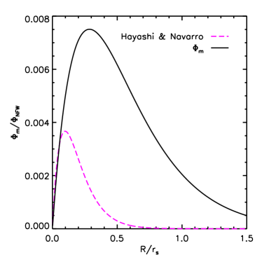
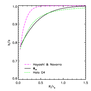
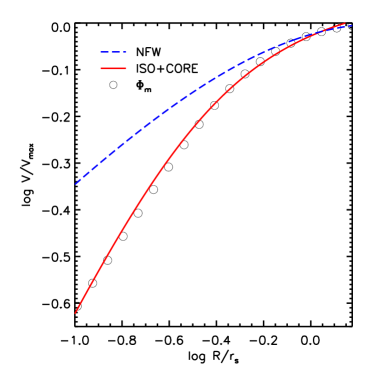
Figure 10: Upper left panel: The potential plotted versus azimuthal angle for halo G4 on a ring of radius $0.5~{}r_{s}$. The potential is well fit by a sinusoidal function whose mean value and amplitude reflect the magnitude of the perturbation relative to a spherically-symmetric potential. Upper right panel: The magnitude of the “perturbing” potential required to yield “core-like” long-slit rotation curves in NFW halos, as presented by Hayashi & Navarro (2006) (dashed curve). The dot-dashed curve corresponds to the perturbation calculated for halo G4, as measured in the plane that contains the major and intermediate axes. The solid curve represents a fit to this perturbation using eq. (9). Lower left panel: Axial ratios of isopotential contours as a function of radius. The dashed, dot-dashed, and solid curves correspond to the HN solution, halo G4, and the fit to halo G4, respectively. Lower right panel: Rotation curve of a disk in the perturbed potential given by the fit to halo G4, produced when a slit samples velocities near the major axis of the disk (open circles). The dashed line shows the circular velocity profile corresponding to the unperturbed, spherically symmetric NFW halo. The solid line shows the best fitting pseudo-isothermal profile with a constant density core.

This is shown by the dashed curve in the upper right panel of Figure 10. The perturbation has a characteristic shape: it increases inwards to a well defined peak that occurs well inside the scale radius of the NFW halo, before decreasing nearer the origin. This behaviour can be approximated by the following fitting formula:

$$\left|\frac{\Phi_{m}}{\Phi_{\rm NFW}}\right|=a_{m}~{}\left({{R}\over{r_{m}}}\right)\exp\left(-\frac{R}{r_{m}}\right),$$ (9)

where $r_{m}\sim 0.098\,r_{s}$ and $a_{m}\sim 9.8\times 10^{-3}$. Note that $r_{m}\ll r_{s}$, as required to affect the rising part of the NFW rotation curve (which peaks at $\sim 2\,r_{s}$), and that the overall perturbation is relatively minor (everywhere less than $0.4\%$).

Is this perturbation consistent with the radially-varying triaxial structure of CDM halos described in the previous section? We calculate $\Phi_{m}$ for a simulated halo with the following procedure. We compute the potential on concentric rings on the plane containing the intermediate and major axes (the most likely one to contain the disk given the alignment between angular momentum and minor axis). The top left panel of Figure 10 shows the potential plotted versus azimuthal angle for halo G4 on a ring of radius $0.5~{}r_{s}$. The potential is periodic in $\pi$ radius, and is reasonably well fit by a sinusoid with three free parameters which describe its phase, amplitude and mean value, i.e., $A\cos(2\phi+\phi_{0})+B$. At each radius, we fit such a sinusoid to the potential and use the best fit parameters to calculate the magnitude of the perturbation, $|\Phi_{m}/\Phi_{\rm NFW}|=|A/B|$. The result is shown for halo G4 as the dot-dashed in the top right panel of Figure 10.

The magnitude of the perturbation peaks at $r\simeq 0.2~{}r_{s}$ and is about $2.5$ times as large as the minimum needed to reconcile a “core-like” rotation curve with a cuspy NFW profile. Unlike the solution presented in HN, however, the magnitude of the perturbation for halo G4 does not decrease to zero at large radii and in this case the closed orbit solutions based on the epicyclic approximation break down. We approximate the perturbation of halo G4 by fitting it over the range $R<0.5~{}r_{s}$ with eq. (9). This fit is shown as the solid line labelled $\Phi_{\rm fit}$ in the top right panel of Figure 10, and the fit parameter value are $a_{m}=0.027$ and $r_{m}=0.21~{}r_{s}$.

The bottom left panel of Figure 10 shows the $b/a$ axial ratio profiles corresponding to halo G4 and the perturbed NFW potential models. The axial ratio profile of the $\Phi_{\rm fit}$ perturbation is quite similar to that of halo G4 and is well fit by eq. (3) with parameter values ($\alpha,r_{\alpha},\gamma$) = $(0.079,0.24~{}r_{s},2.68)$, compared to $(0.062,0.22~{}r_{s},1.85)$ for halo G4.

The lower right panel of Figure 10 shows as open circles the rotation curve that would be obtained by a long slit sampling tangential velocities along the major axis of the disk ($\phi_{a}=0^{\circ}$ in the notation of HN) in the perturbed potential given by the fit to halo G4. The slope of the inner rotation curve is significantly modified from that of the initial NFW profile, and is well fit by a pseudo-isothermal velocity profile (solid line), given by $V_{\rm iso}^{2}(r)=V_{\infty}^{2}[1-({r_{\rm core}}/{r})\tan^{-1}({r}/{r_{\rm core}})]$, where $V_{\infty}$ is the asymptotic velocity and $r_{\rm core}$ is the radius of the constant density core in this model. The best fitting value of the core radius in this case is $r_{\rm core}=0.38~{}r_{s}$, comparable to the characteristic radius of the perturbation, $r_{m}\approx 0.45~{}r_{\alpha}\approx 0.24~{}r_{s}$.

Extending this comparison to the other halos in our simulation suite is not straightforward, because the rather large deviations from spherical symmetry present in many cases preclude the use of the epicyclic approximation to compute closed orbits. Our set of 11 simulations is also too small to allow for a statistically meaningful comparison between simulated halos and LSB rotation curves. The case of G4 is nevertheless encouraging, as it signals that perturbations of the right magnitude and the right shape can result in “core-like” rotation curves such as those observed in some LSB galaxies.

6 Conclusions

We have examined the three-dimensional shape of the gravitational potential in seven Milky Way-sized halos and four dwarf galaxy-sized halos simulated in the concordance $\Lambda$CDM cosmology. We use the ellipsoid fitting method of Springel et al. (2004) to measure the shape of isopotential surfaces as a function of distance from the centre of the halo. The isopotential surfaces are well described by concentric ellipsoids whose principal axes remain aligned across the whole halo, and whose minor axes tend to be parallel to the angular momentum of the halo.

We find that the axial ratios of the isopotential surfaces decrease sharply inwards inside the characteristic scale radius of the halo mass profile, approaching central values of $(c/a)_{0}=0.72\pm 0.04$ and $(b/a)_{0}=0.78\pm 0.08$. The potential becomes more spherical and less axisymmetric from the centre outwards, as $c/a$ increases more gradually than $b/a$. Such radial dependence is well captured by a simple fitting formula, eq. (3), where the characteristic radial scale for $c/a$ is about twice that of $b/a$. Incorporating the radial variation in shape in models of CDM halos represents a significant improvement over the analytic halo potentials generally implemented in N-body simulations.

We use the analytic closed loop orbit solutions presented in Hayashi & Navarro (2006) to investigate the kinematics of thin, filled gaseous disks embedded in such halos. We find that the radially-dependent ellipticity of the potential on the principal planes of the halo generally resembles the perturbation needed to reconcile “core-like” rotation curves with cuspy halo profiles. The amplitude of the ellipticity in the potential is typically larger than needed to obtain linearly-rising long-slit rotation curves according to the treatment presented in HN.

This is important, as the simulations do not include baryons, and the assembly of a baryonic disk will tend to circularize the potential, by (i) inducing changes in the actual mass distribution of the dark halo (Dubinski, 1994; Gustafsson et al., 2006, Abadi et al, in preparation), and by (ii) “opposing” the halo ellipticity—the disk would itself be elliptical but rotated by 90^o relative to the halo potential. The magnitude of the corrections implied by these two effects is at present quite uncertain, and will require simulations more precisely tailored to reproducing the formation of a system with the observed properties of an LSB galaxy.

Because of these uncertainties it would be premature to conclude that halo triaxiality is the main cause of both the wide variety in LSB rotation curve shapes and the existence of rotation curves suggestive of the presence of constant-density cores (Hayashi et al., 2004). Still, our results demonstrate that radially-varying ellipsoidal potentials are expected to be the rule rather than the exception in CDM halos; and indicate that this “natural” feature of CDM halo structure needs to be included in more sophisticated analyses of LSB rotation curves and of other observational probes of the shape of CDM halos.

Table 1: Main parameters of simulated halos

Label	$\epsilon$	$N_{200}$	$M_{200}$	$r_{200}$	$r_{\rm conv}$	$r_{s}$	potential $c/a$			potential $b/a$			mass $c/a$			mass $b/a$
	[$h^{-1}$ kpc]		[$h^{-1}\,M_{\odot}$]	[$h^{-1}$ kpc]	[$h^{-1}$ kpc]	[$h^{-1}$ kpc]	$\alpha$	$r_{\alpha}/r_{s}$	$\gamma$	$\alpha$	$r_{\alpha}/r_{s}$	$\gamma$	$\alpha$	$r_{\alpha}/r_{s}$	$\gamma$	$\alpha$	$r_{\alpha}/r_{s}$	$\gamma$
D1	$0.0625$	$784980$	$7.81\times 10^{9}$	$32.3$	$0.34$	$2.59$	0.052	3.60	1.39	0.024	0.69	0.82	0.15	12.75	0.95	0.08	2.19	0.88
D2	$0.0625$	$778097$	$9.21\times 10^{9}$	$34.1$	$0.37$	$2.43$	0.058	2.87	1.09	0.042	0.73	3.01	0.15	17.69	1.14	0.12	1.42	1.57
D3	$0.0625$	$946421$	$7.86\times 10^{9}$	$32.3$	$0.33$	$2.94$	0.065	3.49	1.00	0.060	1.20	1.22	0.20	12.18	0.78	0.16	3.90	1.42
D4	$0.0625$	$1002098$	$9.72\times 10^{9}$	$34.7$	$0.32$	$2.06$	0.065	3.14	1.54	0.048	2.68	1.90	0.16	9.09	1.34	0.12	6.44	1.57
G1	$0.15625$	$3447447$	$2.29\times 10^{12}$	$214.4$	$1.42$	$23.2$	0.100	1.37	1.27	0.097	0.86	1.76	0.20	9.08	1.04	0.19	2.30	1.56
G2	$0.5$	$4523986$	$2.93\times 10^{12}$	$232.6$	$1.25$	$16.8$	0.075	7.14	1.08	0.066	4.21	0.91	0.19	12.31	2.83	0.16	8.86	1.45
G3	$0.45$	$2661091$	$2.24\times 10^{12}$	$212.7$	$1.65$	$28.0$	0.075	2.24	0.81	0.053	0.87	0.68	0.17	5.04	1.25	0.13	1.56	1.27
G4	$0.3$	$3456221$	$1.03\times 10^{12}$	$164.0$	$1.01$	$12.3$	0.078	0.53	1.00	0.062	0.22	1.85	0.23	1.34	0.81	0.16	0.42	1.29
G5	$0.35$	$3913956$	$1.05\times 10^{12}$	$165.0$	$1.02$	$13.8$	0.059	7.66	0.56	0.019	$\gg 10$	0.07	0.38	0.60	0.77	0.24	1.34	0.93
G6	$0.35$	$3739913$	$9.99\times 10^{11}$	$162.5$	$1.03$	$15.3$	0.078	0.43	1.45	0.066	0.46	1.68	0.21	0.97	1.26	0.16	1.18	1.53
G7	$0.35$	$3585676$	$9.58\times 10^{11}$	$160.3$	$1.02$	$13.4$	0.087	0.92	1.04	0.068	0.41	1.46	0.22	2.34	0.85	0.17	0.76	1.41

References

- Abadi et al. (2006) Abadi M. G., Navarro J. F., Steinmetz M., 2006, Mon. Not. R. Astron. Soc., 365, 747
- Bailin & Steinmetz (2005) Bailin J., Steinmetz M., 2005, Astrophys. J., 627, 647
- Bett et al. (2006) Bett P., Eke V., Frenk C. S., Jenkins A., Helly J., Navarro J., 2006, ArXiv Astrophysics e-prints
- Comerford et al. (2006) Comerford J. M., Meneghetti M., Bartelmann M., Schirmer M., 2006, Astrophys. J., 642, 39
- Crone et al. (1994) Crone M. M., Evrard A. E., Richstone D. O., 1994, Astrophys. J., 434, 402
- de Blok et al. (2001) de Blok W. J. G., McGaugh S. S., Rubin V. C., 2001, Astron. J., 122, 2396
- De Lucia et al. (2004) De Lucia G., Kauffmann G., Springel V., White S. D. M., Lanzoni B., Stoehr F., Tormen G., Yoshida N., 2004, Mon. Not. R. Astron. Soc., 348, 333
- Dubinski (1994) Dubinski J., 1994, Astrophys. J., 431, 617
- Dubinski & Carlberg (1991) Dubinski J., Carlberg R. G., 1991, Astrophys. J., 378, 496
- Fall & Efstathiou (1980) Fall S. M., Efstathiou G., 1980, Mon. Not. R. Astron. Soc., 193, 189
- Fillmore & Goldreich (1984) Fillmore J. A., Goldreich P., 1984, Astrophys. J., 281, 1
- Flores & Primack (1994) Flores R. A., Primack J. R., 1994, Astrophys. J., 427, L1
- Frenk et al. (1988) Frenk C. S., White S. D. M., Davis M., Efstathiou G., 1988, Astrophys. J., 327, 507
- Frenk et al. (1985) Frenk C. S., White S. D. M., Efstathiou G., Davis M., 1985, Nature, 317, 595
- Gunn & Gott (1972) Gunn J. E., Gott J. R. I., 1972, Astrophys. J., 176, 1
- Gustafsson et al. (2006) Gustafsson M., Fairbairn M., Sommer-Larsen J., 2006, ArXiv Astrophysics e-prints
- Hayashi & Navarro (2006) Hayashi E., Navarro J. F., 2006, Mon. Not. R. Astron. Soc., (HN)
- Hayashi et al. (2004) Hayashi E., Navarro J. F., Power C., Jenkins A., Frenk C. S., White S. D. M., Springel V., Stadel J., Quinn T. R., 2004, Mon. Not. R. Astron. Soc., 355, 794
- Helmi (2004) Helmi A., 2004, Mon. Not. R. Astron. Soc., 351, 643
- Hoffman & Shaham (1985) Hoffman Y., Shaham J., 1985, Astrophys. J., 297, 16
- Ibata et al. (2001) Ibata R., Lewis G. F., Irwin M., Totten E., Quinn T., 2001, Astrophys. J., 551, 294
- Jing & Suto (2002) Jing Y. P., Suto Y., 2002, Astrophys. J., 574, 538
- Johnston et al. (2005) Johnston K. V., Law D. R., Majewski S. R., 2005, Astrophys. J., 619, 800
- Katz (1991) Katz N., 1991, Astrophys. J., 368, 325
- Law et al. (2005) Law D. R., Johnston K. V., Majewski S. R., 2005, Astrophys. J., 619, 807
- Mandelbaum et al. (2006) Mandelbaum R., Seljak U., Cool R. J., Blanton M., Hirata C. M., Brinkmann J., 2006, Mon. Not. R. Astron. Soc., 372, 758
- McGaugh & de Blok (1998) McGaugh S. S., de Blok W. J. G., 1998, Astrophys. J., 499, 41
- Moore (1994) Moore B., 1994, Nature, 370, 629
- Navarro et al. (2004) Navarro J. F., Abadi M. G., Steinmetz M., 2004, Astrophys. J., 613, L41
- Navarro et al. (1996) Navarro J. F., Frenk C. S., White S. D. M., 1996, Astrophys. J., 462, 563 (NFW)
- Navarro et al. (1997) Navarro J. F., Frenk C. S., White S. D. M., 1997, Astrophys. J., 490, 493
- Navarro et al. (2004) Navarro J. F., Hayashi E., Power C., Jenkins A. R., Frenk C. S., White S. D. M., Springel V., Stadel J., Quinn T. R., 2004, Mon. Not. R. Astron. Soc., 349, 1039
- Olling & Merrifield (2000) Olling R. P., Merrifield M. R., 2000, Mon. Not. R. Astron. Soc., 311, 361
- Pointecouteau et al. (2005) Pointecouteau E., Arnaud M., Pratt G. W., 2005, Astron. & Astrophys., 435, 1
- Power et al. (2003) Power C., Navarro J. F., Jenkins A., Frenk C. S., White S. D. M., Springel V., Stadel J., Quinn T., 2003, Mon. Not. R. Astron. Soc., 338, 14 (P03)
- Prada et al. (2003) Prada F., Vitvitska M., Klypin A., Holtzman J. A., Schlegel D. J., Grebel E. K., Rix H.-W., Brinkmann J., McKay T. A., Csabai I., 2003, Astrophys. J., 598, 260
- Quinn et al. (1986) Quinn P. J., Salmon J. K., Zurek W. H., 1986, Nature, 322, 329
- Roberts & Whitehurst (1975) Roberts M. S., Whitehurst R. N., 1975, Astrophys. J., 201, 327
- Rubin & Ford (1970) Rubin V. C., Ford W. K. J., 1970, Astrophys. J., 159, 379
- Sackett et al. (1994) Sackett P. D., Rix H.-W., Jarvis B. J., Freeman K. C., 1994, Astrophys. J., 436, 629
- Springel et al. (2004) Springel V., White S. D. M., Hernquist L., 2004, in Ryder S., Pisano D., Walker M., Freeman K., eds, IAU Symposium The shapes of simulated dark matter halos. p. 421
- Teuben (1991) Teuben P. J., 1991, in Casertano S., Sackett P. D., Briggs F. H., eds, Warped Disks and Inclined Rings around Galaxies Velocity Fields of Disks in Triaxial Potentials. p. 40
- Thomas et al. (1998) Thomas P. A., Colberg J. M., Couchman H. M. P., Efstathiou G. P., Frenk C. S., Jenkins A. R., Nelson A. H., Hutchings R. M., Peacock J. A., Pearce F. R., White S. D. M., 1998, Mon. Not. R. Astron. Soc., 296, 1061
- van den Bosch et al. (2002) van den Bosch F. C., Abel T., Croft R. A. C., Hernquist L., White S. D. M., 2002, Astrophys. J., 576, 21
- Warren et al. (1992) Warren M. S., Quinn P. J., Salmon J. K., Zurek W. H., 1992, Astrophys. J., 399, 405
- Zwicky (1933) Zwicky F., 1933, Helvetica Phys. Acta, 6, 110