Oscillation effects on high-energy neutrino fluxes from astrophysical hidden sources

Abstract

High-energy neutrinos are expected to be produced in a vareity of astrophysical sources as well as in optically thick hidden sources. We explore the matter-induced oscillation effects on emitted neutrino fluxes of three different flavors from the latter class. We use the ratio of electron and tau induced showers to muon tracks, in upcoming neutrino telescopes, as the principal observable in our analysis. This ratio depends on the neutrino energy, density profile of the sources and on the oscillation parameters. The largely unknown flux normalization drops out of our calculation and only affects the statistics. For the current knowledge of the oscillation parameters we find that the matter-induced effects are non-negligible and the enhancement of the ratio from its vacuum value takes place in an energy range where the neutrino telescopes are the most sensitive. Quantifying the effect would be useful to learn about the astrophysics of the sources as well as the oscillation parameters. If the neutrino telescopes mostly detect diffuse neutrinos without identifying their sources, then any deviation of the measured flux ratios from the vacuum expectation values would be most naturally explained by a large population of hidden sources for which matter-induced neutrino oscillation effects are important.

I Introduction

High-energy ($\gtrsim 100$ GeV) neutrino emission has been predicted from several types of astrophysical sources such as active galactic nuclei (AGNs), gamma-ray bursts (GRBs), core-collapse supernovae (SNe), supernova remnants (SNRs), microquasars, etc. Dermer:2006xt . All these sources have been observed in electromagnetic wave bands ranging from radio to high-energy $\gamma$-rays. Low energy ($\sim 10$ MeV) thermal neutrinos have been detected from a nearby core-collapse SN 1987A Hirata:1987hu . High-energy neutrinos may be detected from a much longer distance because of an increasing interaction cross-section with energy Frichter:1994mx ; gqrs ; Gandhi:1998ri . Upcoming kilometer scale ice/water Cherenkov detectors such as IceCube Achterberg:2006md in Antarctica and its counterpart in the Mediterranean, called KM3NeT Katz:2006wv , will thus open up a new observation window in high-energy neutrinos.

Neutrinos, unlike their electromagnetic counterparts, may carry information on temperature, density, etc. from deep inside the astrophysical sources. Their detection may also be used to probe neutrino flavor oscillation parameters in matter and in vacuum as they propagate inside the sources and over astrophysical distances to reach Earth. The results will be complementary to accelerator and reactor based experiments. Particular examples have been carried out in detail for $\sim 10$ MeV thermal neutrinos from core-collapse SNe Dighe:1999bi .

Oscillations of high energy neutrinos have also been extensively discussed in Refs. Rodejohann:2006qq ; Winter:2006ce ; Serpico:2005sz ; serpico ; Costantini:2004ap ; Xing:2006uk ; Cirelli:2005gh ; Fogli:2006jk ; lunardinismirnov . The sensitivity of high energy neutrinos to oscillation parameters has been explored in Refs. Rodejohann:2006qq ; Winter:2006ce ; Serpico:2005sz ; serpico ; Costantini:2004ap ; Xing:2006uk Matter effects in the context of neutrinos from dark matter annihilation have been considered in Ref. Cirelli:2005gh . Oscillations of solar atmosphere neutrinos have been discussed in Ref. Fogli:2006jk . Matter effects for high energy neutrinos are generally small. In order to get significant effects it is necessary to encounter a resonant density, as well as to go through a minimum matter width, as shown in Ref. lunardinismirnov . These conditions are usually not satisfied for optically thin sources.

In this paper we explore flavor oscillation effects on high-energy neutrinos from optically thick sources where matter effects can be larger. These neutrinos are produced deep inside the astrophysical sources (so-called “hidden sources”) and as such their emission from the source is not accompanied by any high-energy electromagnetic component. Examples of hidden sources may be highly relativistic GRB jets as they are formed inside collapsed stars and start burrowing their way through the stellar envelope Meszaros:2001ms ; Razzaque:2003uv ; semi-relativistic jets inside core-collapse SNe which may impact and disrupt the envelope but choke inside Razzaque:2004yv ; and core dominated AGNs Alvarez-Muniz:2004uz ; Stecker:2005hn . The first two cases are motivated by the observation of a number of GRBs associated with supernovae which supports the collapsar model of GRBs MWH01 . The collapsar model ties the GRBs and supernovae in a common thread, both originating from core-collapse of massive stars. While observed GRBs are endowed with highly relativistic jets, many more such collapses are expected to produce mildly relativistic jets. In both cases the jet is launched from inside the star MWH01 ; MR01 ; WM03 and burrows through the stellar interior while the envelope is still intact. High energy neutrinos, produced by collisions of plasma materials (so called “internal shocks”) in the jet, are emitted following a density gradient while the jet itself may or may not break through the envelope. High-energy neutrinos are produced via decays of pions and kaons created by hadronic ($pp$) and/or photo-hadronic ($p\gamma$) interactions of shock-accelerated protons in these examples. We concentrate on matter enhancement of the electron (anti)neutrino flux due to the small mixing angle $\theta_{13}$ as these neutrinos propagate to the stellar surface from their production site. Matter effects have not been previously discussed for these sources and they provide an opportunity for identifying and studying such “hidden”sources through the neutrinos they emit. We show in particular the energy range where this effect may be detectable by neutrino telescopes, and we also comment on possible extraction of neutrino properties such as mass hierarchy and the CP violation phase.

The organization of the paper is as follows: We outline the astrophysical source model and neutrino flux parametrization in Sec. II. We discuss neutrino oscillations, our numerical approach to calculate the effects and analytic expectations in Sec. III. Detection and our results are given in Sec. IV and in Sec. V respectively. Conclusions and outlooks are given in Sec. VI.

II Astrophysics of the source

The particular hidden source model we employ for calculation purpose is a jetted core collapse supernova model in Ref. Razzaque:2004yv . Our treatment may however be applied to any generic case of a neutrino flux and matter density profile. The presupernova star is a blue supergiant (BSG) with a radiative hydrogen envelope which is capable to produce a Type II or Ib SN. The hydrogen envelope sits on a helium core of radius $r_{\rm He}\sim 10^{11}$ cm. In case of significant stellar mass loss, the presupernova stars may have no hydrogen envelope left at all and produce Type Ic SNe, a fraction of which are now strongly believed to produce GRBs as well. However, we do not investigate this case as the relativistic jet front ($r_{\rm jet}\sim 10^{10.8}$ cm) is too close to the stellar surface to have any significant amount of material in front Razzaque:2004yv .

An analytic form of the density distribution near the edge of each layer of a star with polytropic structure is given by $\rho=\rho_{1}(R_{\star}/r-1)^{n}$ matzmckee99 . Here $R_{\star}$ is the star’s radius and the polytropic index $n=3$ for a radiative envelope with constant Thomson opacity. For a helium star of $R_{\star}\approx 10^{11}$ cm, $\rho_{1}\approx 2$ g cm^-3 and $n=3$ were found by fitting data from SN 1998bw wooslangweav93 . The presupernova star of SN 1987A is a BSG with $R_{\star}\approx 3\cdot 10^{12}$ cm, $\rho_{1}\approx 3\cdot 10^{-5}$ g cm^-3 and $n=3$ shignom90 ; arnett91 . Below we write 3 models of the density profile that we use for a BSG of $R_{\star}=3\cdot 10^{12}$ cm. All models are normalized to give the same density $\rho=2(10^{11}/10^{10.8}-1)^{3}=0.4$ g cm^-3, as in the case of a helium star, at $r=r_{\rm jet}=10^{10.8}$ cm.

Model [A] corresponds to a polytropic hydrogen envelope with $\rho(r)\propto r^{-3}$, scaling valid in the range $r_{\rm jet}\lesssim r\lesssim R_{\star}$. Model [B] is a power-law fit with an effective polytropic index $n_{\rm eff}=17/7$ as done for SN 1987A in Ref. chevsok89 . Model [C] includes a sharp drop in density at the edge of the helium core. Note that our choice of different $n_{\rm eff}$ below and above the helium core, in this case, is motivated by Ref. matzmckee99 . The parameter ${\cal A}$ corresponds to the drop in density and its value is set by hand.

$${\rm[A]}~{}~{}\rho(r) = 4.0\cdot 10^{-6}\left(\frac{R_{\star}}{r}-1\right)^{3}~{}{\rm g~{}cm}^{-3}$$ (1)

$${\rm[B]}~{}~{}\rho(r) = 3.4\cdot 10^{-5}\times\begin{cases}(R_{\star}/r)^{17/7}~{};~{}10^{10.8}~{}{\rm cm}<r<r_{b}=10^{12}~{}{\rm cm}\cr(R_{\star}/r_{b})^{17/7}(r-R_{\star})^{5}/(r_{b}-R_{\star})^{5}~{};~{}r>r_{b}\end{cases}~{}{\rm g~{}cm}^{-3}$$ (2)

$${\rm[C]}~{}~{}\rho(r) = 6.3\cdot 10^{-6}{\cal A}\left(\frac{R_{\star}}{r}-1\right)^{n_{\rm eff}}~{}{\rm g~{}cm}^{-3}~{};~{}(n_{\rm eff},{\cal A})=\begin{cases}(2.1,20)~{};~{}10^{10.8}~{}{\rm cm}<r<10^{11}~{}{\rm cm}\cr(2.5,1)~{};~{}r>10^{11}~{}{\rm cm}\end{cases}$$ (3)

We have plotted the density profiles in Eqs. (1), (2) and (3) in Fig. 1. The number density of electrons is given by $N_{e}(r)=N_{A}\rho(r)Y_{e}$, where $Y_{e}\approx 1$ in our cases, is the number of electrons per nucleon or the electron fraction. As for reference, $N_{e}=2.4\cdot 10^{23}$ cm^-3 at $r=r_{\rm jet}=10^{10.8}$ cm for all models described above.

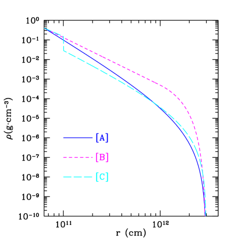
Figure 1: (Color online) Models of outer density profile of a blue supergiant star of radius $R_{\star}=10^{12.5}$ cm. The outermost hydrogen envelope sits on a helium envelope extending up to a radius of $\sim 10^{11}$ cm. High-energy neutrinos are produced at a radius $r_{\rm jet}=10^{10.8}$ cm by a relativistic jet. The models [A], [B] and [C] are described in Eqs. (1), (2) and (3) respectively.

We use the pion and kaon decay neutrino flux models from hadronic ($pp$) interactions by shock accelerated protons in the semi-relativistic hidden jets Razzaque:2004yv ; Ando:2005xi . The fluxes ($\Phi_{\nu_{\mu}}=\Phi_{\bar{\nu}_{\mu}}=2\Phi_{\nu_{e}}=2\Phi_{\bar{\nu}_{e}}$), from an isolated source, at the production site $r=r_{\rm jet}$ may be parametrized as rmw05

$$\Phi_{\pi,\nu_{\mu}}^{\rm s} = 4\cdot 10^{45}\left(\frac{d_{L}}{\rm cm}\right)^{-2}\left(\frac{E_{\nu}}{300~{}{\rm GeV}}\right)^{-4}$$ (4)

$$~{}{\rm GeV}^{-1}{\rm cm}^{-2}{\rm s}^{-1}~{};~{}$$

$$~{}100\lesssim E_{\nu}/{\rm GeV}\lesssim 3\cdot 10^{5},$$

$$\Phi_{K,\nu_{\mu}}^{\rm s} = 8\cdot 10^{38}\left(\frac{d_{L}}{\rm cm}\right)^{-2}\left(\frac{E_{\nu}}{5\cdot 10^{4}~{}{\rm GeV}}\right)^{-\kappa}$$ (5)

$$~{}{\rm GeV}^{-1}{\rm cm}^{-2}{\rm s}^{-1}~{};~{}$$

$$~{}\kappa=\begin{cases}3~{};~{}100\lesssim E_{\nu}/{\rm GeV}\lesssim 5\cdot 10^{4}\cr 4~{};~{}5\cdot 10^{4}\lesssim E_{\nu}/{\rm GeV}\lesssim 3\cdot 10^{5},\end{cases}$$

respectively from pion and kaon decays. Here $d_{L}$ is the luminosity distance of the source. Next we discuss oscillation effects on these neutrinos as they propagate from inside the stellar interior to the surface in dense media, from the source to Earth and through the Earth. Note that high energy neutrinos are produced in shocked material in the jet which has a density lower than the surrounding stellar material. However, the width of the shock is too small (jet radius divided by the Lorentz boost factor of the jet) to have any significant oscillation effect before the neutrinos start moving through the jet head (which is roughly in equilibrium with surrounding material) and the envelope. Also, the jet is well outside the stellar core which may be turbulent and the envelope is not disrupted yet.

III Neutrino oscillation in vacuum and in matter

Solar, atmospheric, accelerator and reactor neutrinos have provided ample evidence for neutrino oscillations. Neutrinos from astrophysical sources like those described above are affected by oscillations, which change the flavor composition of the fluxes between production and detection.

The neutrino flavor eigenstates $\nu_{\alpha}$, where $\alpha=e,\mu,\tau$ in the case of 3 flavor mixing, are related to the mass eigenstates $\nu_{j}$, where $j=1,2,3$ corresponding to the masses $m_{j}$, by the Maki-Nakagawa-Sakata (MNS) unitary mixing matrix $U$ as $\nu_{\alpha}=U_{\alpha j}\nu_{j}$. The sum over repeated indices is implied. We use the standard expression of $U$ from Ref. pdg04 .

We use standard oscillation parameters obtained from global fits to neutrino oscillations data:

$$\Delta m^{2}_{\rm sol} = \Delta m^{2}_{21}\sim 8\times 10^{-5}\hbox{ eV}^{2}$$

$$\theta_{\rm sol} = \theta_{12}\sim 33.83^{\circ}$$

$$|\Delta m^{2}_{\rm atm}| = |\Delta m^{2}_{32}|\sim 2.4\times 10^{-3}\hbox{ eV}^{2}$$

$$\theta_{\rm atm} = \theta_{23}\sim 45^{\circ}$$

$$\sin^{2}(2\theta_{13}) \buildrel<\over{{}_{\sim}} 0.15$$ (6)

The sign of the atmospheric mass difference has not been determined. Positive (negative) $\Delta m^{2}_{\rm atm}$ correspond to the normal (inverted) hierarchies.

Uncertainties in the oscillation parameters are still relatively large and small variations due to these uncertainties on the generic results we present here are to be expected. We will explore the impact of the expected errors of the oscillation parameters on our observable and we will discuss how these errors could affect an eventual measurement of the neutrino mass hierarchy (i.e normal vs inverted) via matter effects.

We will also consider the effects of a CP violating phase which is at present unconstrained. A precise approximation (for constant density and energies high enough such that $\Delta_{21}/V_{e}\ll 1$ and $\Delta_{21}L\ll 1$) for the $\nu_{e}\rightarrow\nu_{\mu}$ transition probability is given by golden :

$$P_{\nu_{e}\nu_{\mu}(\bar{\nu}_{e}\bar{\nu}_{\mu})}=$$

$$\sin^{2}\theta_{23}\sin^{2}2\theta_{13}\left(\frac{\Delta_{31}}{\tilde{V}_{\mp}}\right)^{2}\sin^{2}\left(\frac{\tilde{V}_{\mp}L}{2}\right)$$

$$+\cos^{2}\theta_{23}\sin^{2}2\theta_{12}\left(\frac{\Delta_{21}}{V_{e}}\right)^{2}\sin^{2}\left(\frac{V_{e}L}{2}\right)$$ (7)

$$+\tilde{J}\frac{\Delta_{21}}{V_{e}}\frac{\Delta_{31}}{\tilde{V}_{\mp}}\sin\left(\frac{V_{e}L}{2}\right)\sin\left(\frac{\tilde{V}_{\mp}L}{2}\right)\cos\left(\pm\delta-\frac{\Delta_{31}L}{2}\right)~{},$$

where $\Delta_{ij}=\Delta m^{2}_{ij}/2E_{\nu}$, $\tilde{V}_{\mp}\equiv|V_{e}\mp\Delta_{31}|$, the matter potential $V_{e}=V_{e}(r)$, $\tilde{J}$ is the Jarslog invariant and the sign minus (plus) refers to neutrinos (antineutrinos).

For the above values of $\Delta m^{2}$, even for the high energies of interest here, the distances relevant for the sources described above are so large that, after propagation through vacuum, only the averaged oscillation is observable for the simple two flavor case with the probability given by

$$P(\nu_{\alpha}\to\nu_{\beta})=\sin^{2}(2\theta)\sin^{2}\left(\frac{\Delta m^{2}L}{4E}\right)\longrightarrow\!\!\!\!\!\!\!\!\!\!\!\!{}_{{}_{{}_{L\to\infty}}}\frac{1}{2}\sin^{2}(2\theta)\,.$$ (8)

In the three flavor case, given fluxes at the surface of the source $\phi^{0}_{\nu_{e}}$, $\phi^{0}_{\nu_{\mu}}$ and $\phi^{0}_{\nu_{\tau}}$, the fluxes at Earth are given by:

$${}\!\!\!\phi_{\nu_{e}}\!\!\! = \!\!\!\phi^{0}_{\nu_{e}}-\frac{1}{4}\sin^{2}2\theta_{12}(2\phi^{0}_{\nu_{e}}-\phi^{0}_{\nu_{\mu}}-\phi^{0}_{\nu_{\tau}})$$ (9)

$$\!\!\!\phi_{\nu_{\mu}}\!\!\! = \!\!\!\phi_{\nu_{\tau}}\!\!=\!\!\frac{1}{2}(\phi^{0}_{\nu_{\mu}}+\phi^{0}_{\nu_{\tau}})+\frac{1}{8}\sin^{2}2\theta_{12}(2\phi^{0}_{\nu_{e}}-\phi^{0}_{\nu_{\mu}}-\phi^{0}_{\nu_{\tau}})$$

if we assume that $\theta_{23}$ is maximal and $\theta_{13}$ is very small (as indicated by neutrino oscillation data). If neutrinos are produced in pion and/or kaon decays, the initial flavor ratio is given by $\nu_{e}:\nu_{\mu}:\nu_{\tau}=1:2:0$. After propagation over very long distances in vacuum, neutrino oscillations change this ratio to $1:1:1$ because of the maximal $\nu_{\mu}\leftrightarrow\nu_{\tau}$ mixing. For the sources we are considering, in the low energy range, even the distance traveled inside the source is large enough that neutrinos oscillate many times and the phase information is lost. When the initial ratio $\nu_{e}:\nu_{\mu}:\nu_{\tau}$ is different from $1:2:0$, the flavor ratio at Earth is affected by the full three flavor mixing and is different from $1:1:1$.

In the case of interest here, even though neutrinos are produced by pion and kaon decays, the fluxes at Earth can have a flavor composition quite different from the standard $1:1:1$ ratio. This is because the neutrino flavor composition is affected by the propagation through matter inside the astrophysical object.

The fluxes at the surface of the star are given by the sum of products of the fluxes at the production site [Eqs.(4) and (5)] and the oscillation probabilities as

$$\phi^{0}_{\nu_{e}} = \phi^{\rm s}_{\nu_{e}}P(\nu_{e}\to\nu_{e})+\phi^{\rm s}_{\nu_{\mu}}P(\nu_{\mu}\to\nu_{e})$$

$$= \phi^{\rm s}_{\nu_{\mu}}\left(\frac{1}{2}P(\nu_{e}\to\nu_{e})+P(\nu_{\mu}\to\nu_{e})\right)$$

$$\phi^{0}_{\nu_{\mu}} = \phi^{\rm s}_{\nu_{\mu}}\left(\frac{1}{2}P(\nu_{e}\to\nu_{\mu})+P(\nu_{\mu}\to\nu_{\mu})\right)$$

$$\phi^{0}_{\nu_{\tau}} = \phi^{s}_{\nu_{\mu}}\left(\frac{1}{2}P(\nu_{e}\to\nu_{\tau})+P(\nu_{\mu}\to\nu_{\tau})\right)$$ (10)

The same type of relations apply to anti-neutrinos.

The $\nu_{\alpha}\leftrightarrow\nu_{\beta}$ oscillation probabilities $P_{\alpha\beta}$ on the stellar surface $r=R_{\star}$ can be obtained by solving, with the appropriate initial conditions, the evolution equation:

$$i\frac{d}{dr}\left(\begin{array}[]{c}\nu_{e}\\ \nu_{\mu}\\ \nu_{\tau}\end{array}\right)=\left[\frac{1}{2E}U\left(\begin{array}[]{ccc}0&0&0\\ 0&\Delta m_{21}^{2}&0\\ 0&0&\Delta m_{31}^{2}\end{array}\right)U^{\dagger}+\left(\begin{array}[]{ccc}V_{e}(r)&0&0\\ 0&0&0\\ 0&0&0\end{array}\right)\right]\left(\begin{array}[]{c}\nu_{e}\\ \nu_{\mu}\\ \nu_{\tau}\end{array}\right).$$ (23)

Here $V_{e}(r)=\sqrt{2}G_{F}N_{e}(r)$ is the matter-induced charged current potential for $\nu_{e}$ in a medium of electron number density $N_{e}(r)$ found from Eqs. (1), (2) and (3). For $\bar{\nu}_{e}$ the potential changes sign.

Matter effects are expected to be large when neutrinos go through a resonant density. For constant electron density, there would be two such resonances, corresponding to the two mass squared differences:

$$N_{e}^{L} = \frac{\Delta m^{2}_{\rm sol}\cos 2\theta_{12}}{2\sqrt{2}G_{F}E}\simeq\frac{3\times 10^{23}}{E[GeV]}{\rm cm}^{-3}$$ (24)

$$N_{e}^{H} = \frac{|\Delta m^{2}_{\rm atm}|\cos 2\theta_{13}}{2\sqrt{2}G_{F}E}\simeq\frac{9\times 10^{24}}{E[GeV]}{\rm cm}^{-3}$$ (25)

As can be seen from the previous section, these densities can be encountered in the sources of interest by neutrinos with the relevant energies.

Even if $\theta_{13}$ is very small, matter effects can be expected from the solar $\Delta m^{2}$ oscillations [see Eq. (24)]. If $\theta_{13}$ is non-negligible, larger matter effects can be expected from the atmospheric $\Delta m^{2}$ oscillations [see Eq. (25)]. These are non-negligible at a relatively higher energy.

Since the matter potential is different for anti-neutrinos, it is important to independently solve the evolution equations for neutrinos and anti-neutrinos and consider the averaging over the two fluxes only when reaching the detector, which cannot distinguish between the two. Note that if the hierarchy is normal (inverted) the resonant behavior occurs only in the neutrino (anti-neutrino) channel.

The matter density in the sources we are considering is varying rather strongly, such that a resonance is not directly observable. Adiabatic conditions are not usually satisfied, such that a full numerical treatment of the problem is necessary. The adiabatic approximation can still be used in some energy range. It is useful to understand some of the features introduced by matter effects by analyzing limiting regions of the models described in the previous section. The adiabaticity parameter is defined as (see Ref. Dighe:1999bi and references therein):

$$\gamma\equiv\frac{\Delta m^{2}}{2E}\frac{\sin^{2}2\theta}{\cos 2\theta}\frac{1}{(1/N_{e})(dN_{e}/dr)}~{},$$ (26)

i.e. the ratio of the resonance width and the neutrino oscillation length. In other words, the adiabaticity parameter represents the number of oscillations that occur in the resonance region. Adiabatic transition ($\gamma\gg 1$) means that the neutrino will remain in its particular superposition of initial instantaneous mass eigenstates as it crosses the resonance. The “flip” probability, that is, the probability that a neutrino in one matter eigenstate jumps to the other matter eigenstate is

$$P_{\rm flip}=\exp\left(-\frac{\pi}{2}\gamma\right)~{},$$ (27)

which means that, if the neutrino adiabaticity parameter is $\gamma\gg 1$, the “flip” probability $P_{\rm flip}\simeq 0$, many oscillations will take place at the resonance region and strong flavor transition will occur. On the other hand, if the adiabaticity parameter is $\gamma\geq 1$, only a few oscillations take place in the resonant region and the mixing between instantaneous matter eigenstates is important, and $P_{\rm flip}$ gives the jumping probability from one instantaneous mass eigenstate to another. For the solar transition, where the mixing angle is large, the appropriate expressions for the adiabaticity conditions and flip probabilities can be found in flipsolar . Since the main effects that we are interested in correspond to the small mixing angle, we limit our analitical discussion to this case. We would like to emphasize that in order to obtain the correct neutrino oscillation probabilities a full numerical treatment of the problem is necessary and our discussion based on flip probability serves only as a qualitative guide to understanding the solution in some limited energy ranges where adiabaticity is satisfied.

Figure 2 shows the flip probability corresponding to the atmospheric transition for the three density profiles we consider.

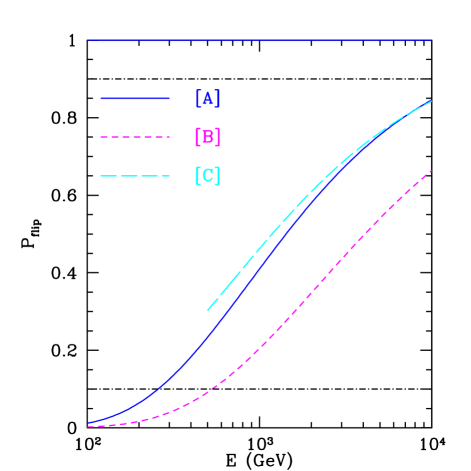
Figure 2: (Color online) Flip probability corresponding to the atmospheric transition for $\sin^{2}2\theta_{13}=0.15$, for the three density profiles in Fig. 1.

We explicitly delimit three different regions: the adiabatic region corresponds to very small flip probabilities ($P_{\rm flip}<0.1$) and strong flavor transitions; in the intermediate region ($0.1<P_{\rm flip}<0.9$) the transitions are not complete; the highly non-adiabatic region corresponds to very high flip probabilities ($P_{\rm flip}>0.9$).

At low energies transitions are adiabatic for the density profiles in models [A] and [B], so strong conversion is expected for these two models. Model [C] has a sharp drop in density and at energies below 500 GeV the resonant density is reached only on the step, where it is highly non-adiabatic, so one does not expect a significant matter enhancement.

At higher energies the adiabatic regime applies only for Model [B], for which oscillation effects are expected to be large, while for models [A] and [C] the flavor transition is incomplete and a smaller effect is expected. These expectations are confirmed by our exact results, that is, around energies $\sim 1$ TeV, the effect for the Model [A] and the Model [C] should be similar and smaller than the one observed for the Model [B]. The differences in the adiabaticity behavior for the three models are induced by their different matter profiles, see Fig. 1: for Model [B] (which has the least steep matter density), the adiabaticity condition is satisfied for a larger neutrino energy range. The adiabaticity of the transitions depends on the matter density profile. If this is very steep, the corresponding resonance width will be very small (it is inversely proportional to the derivative of the matter potential) and consequently the neutrino system can not adapt itself, only a few oscillations will take place and the flavor transitions will not be complete. In order to have large matter effects it is also necessary to go through a minimum matter width, as shown in Ref. lunardinismirnov . For the sources we consider here the density is high enough that this condition is satisfied.

In Fig. 3 we show the electron, muon and tau neutrino fluxes at the surface of the source, normalized to the initial electron neutrino fluxes. We compare the case when only the vacuum oscillations are considered inside the source with the fluxes of neutrinos when matter effects are taken into account with a density profile as in Model [A] or Model [B], for normal hierarchy. The averaging due to fast vacuum oscillations can already be observed in the lower energy range. It can also clearly be seen that matter effects modify the flavor composition of the neutrino fluxes, introducing energy-dependent features. As expected from the discussion above, the effects are larger for Model [B] where adiabatic-like transitions occur in a wider energy range. We also show the corresponding anti-neutrino fluxes for Model [A] for comparison. The results are very close to those in vacuum, as expected for the normal hierarchy.

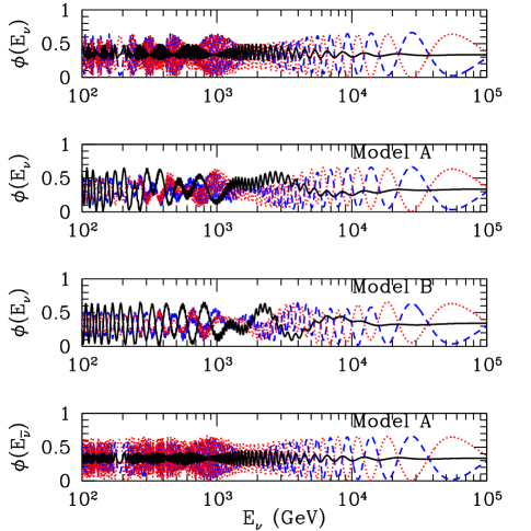
Figure 3: (Color online) Neutrino fluxes at the surface of the source (for $\sin^{2}2\theta_{13}=0.15$), normalized to the initial electron neutrino fluxes. From upper to lower panels: vacuum, Model [A], Model [B] and Model [A] antineutrinos. The solid, dashed and dotted curves are for $\nu_{e}$, $\nu_{\mu}$ and $\nu_{\tau}$ respectively.

After propagating the neutrinos through matter to the surface of the star, the fluxes at Earth immediately follow by considering the averaged oscillations over the long travel distance in vacuum as obtained from Eq. (III).

Figure 4 makes the same comparison presented in Fig. 3 after propagation all the way to the Earth. The flavor composition of the neutrinos gets further modified by the propagation from the source to the Earth.

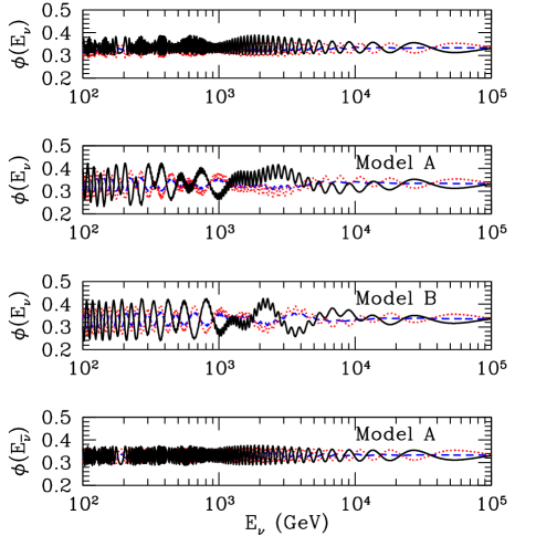
Figure 4: (Color online) Same as Fig. 3, but at the surface of the Earth.

IV Detection

On their way to detectors, neutrinos also propagate through matter in the Earth. In this case matter effects on neutrino oscillations are however extremely small, since the energies considered here are much higher than the resonant energy inside the Earth. For $\Delta m^{2}_{\rm atm}=2.4\times 10^{-3}$ eV² the corresponding resonant energy for a neutrino going through the Earth’s mantle (with the density $\sim 3$ g/cm³) is around 10 GeV, already lower than the energies we consider. The resonant energy is even lower for the solar mass difference or for trajectories going through the higher density Earth core MS .

The charged current and neutral current neutrino-nucleon interaction cross-section increases with energy and attenuation effects start becoming important for the propagation through matter. The interaction length:

$${\cal L}=\frac{1}{\sigma_{\nu N}(E)N_{A}}$$ (28)

becomes comparable to the Earth diameter around 40 TeV. The attenuation effects are thus becoming relevant only at the highest energies considered here, where the fluxes are very small. Consequently, propagation through the Earth will have negligible effects on the neutrino fluxes and flavor composition previously discussed.

Neutrinos from the sources discussed here are expected to be detectable in IceCube and other neutrino telescopes which have good sensitivity in the energy range of interest, between 100 GeV and 100 TeV.

It is possible in IceCube to get information about the flavor composition of the neutrinos as well. The detector is mostly sensitive to observing muons identified by their very long tracks, thus counting the number of $\nu_{\mu}$ interactions. Electron neutrino interactions create electromagnetic cascades which can be observed in IceCube. Tau neutrinos will also lead to cascades. At these energies the tau decay length is very small and the interaction of the neutrino and tau decay cannot be separated. It might be possible to separately infer the fluxes of all three flavors if hadronic showers can be well separated from electromagnetic showers through their muon track content. We will consider taus to be indistinguishable from electrons in our analysis and we will compare the number of tracks due to $\nu_{\mu}$ and number of showers due to $\nu_{e}$ and $\nu_{\tau}$.

Another important feature of interest for the detection of the effects studied in this paper is the energy dependence of the signal: as discussed in the previous section, matter effects have a strong dependence on energy, which is correlated with the density profile inside the source; changes in neutrino oscillation parameters also induce energy dependent effects, as we discuss in more detail in the next section. The energy resolution in IceCube is expected to be somewhat better than 30% on a logarithmic scale for muon neutrinos and about 20% on a linear scale for cascades.

We explore the spectral shape of the shower-to-muon track ratio inferred at Icecube, defined as:

$$R=\frac{N_{\nu_{e}}+N_{\bar{\nu}_{e}}+N_{\nu_{\tau}}+N_{\bar{\nu}_{\tau}}}{N_{\nu_{\mu}}+N_{\bar{\nu}_{\mu}}}~{}.$$ (29)

The absolute flux normalization thus does not affect our results. The number of events, $N_{\nu_{\alpha}(\bar{\nu}_{\alpha})}$ is proportional to:

$$N_{\nu_{\alpha}(\bar{\nu}_{\alpha})}\sim\int_{\Delta E_{\nu}}(\phi^{\pi}_{\nu_{\alpha}(\bar{\nu}_{\alpha})}+\phi^{K}_{\nu_{\alpha}(\bar{\nu}_{\alpha})})(E_{\nu})\times\sigma_{\nu_{\alpha}(\bar{\nu}_{\alpha})}(E_{\nu})dE_{\nu}~{},$$ (30)

i.e. we have computed the (anti)neutrino fluxes from pion and kaon decays at the detector after considering the propagation inside the source (affected by matter effects) as well as the propagation from the source to the detector. The (anti)neutrino fluxes are then convoluted with the (anti)neutrino cross-sections gqrs and integrated over the neutrino energy, assuming a conservative energy bin size of $\Delta E_{\nu}=0.3E_{\nu}$. If the matter potential inside the astrophysical source is neglected, the neutrino flavor ratio in Eq. (29) should be almost constant, $R\simeq 2$, over all the neutrino energy range. Adding the matter contribution to the neutrino propagation will change this constant value of $R$ in an energy dependent fashion. In the following section we explore the spectral behavior of the shower-to-track ratio in the 300 GeV- 300 TeV neutrino energy range, considering both normal and inverted neutrino mass orderings and exploring the effects of a non zero leptonic CP violating phase $\delta$ and of uncertainties in other oscillation parameters.

V Spectral Analysis

We present here the main results of our study. We are mainly interested in neutrino propagation through matter inside the source. This is followed by the propagation through vacuum between the source and Earth. Matter effects and absorption inside the Earth are negligible for the energies considered here. As discussed in the previous section, a good observable for studying the effects of neutrino propagation inside the source is the spectral shape defined in Eq. (29). While $R\simeq 2$ for the optically thin sources, energy dependent deviations from this value are expected due to matter effects in the astrophysical hidden sources considered here.

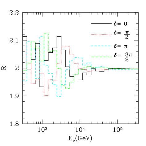
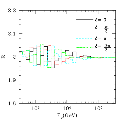
Figure 5: (Color online) The upper (lower) panel depicts the shower-to-muon track ratio defined in Eq. (29) for $\sin^{2}2\theta_{13}=0.15$, for Model [A], for the case of normal (inverted) hierarchy and for different values of the CP violating phase $\delta$.

Figure 5 shows the shower-to-muon track ratio in Eq. (29) for the normal and inverted neutrino mass hierarchies for the Model [A] density profile [see Eq. (1)]. Deviations from the standard scenario are non-negligible in the energy range around a few TeV. The impact of the matter potential is much larger if nature has chosen the normal mass ordering, since, if that is the case, only neutrinos can go through the resonance density $N^{H}_{e}$ and the effect will be larger due to the higher neutrino cross-section, when compared to the antineutrino one. For neutrino energies $E_{\nu}<6$ TeV, where the resonant effect in the (anti)neutrino propagation is expected to be located, the neutrino cross-section is roughly twice the antineutrino cross section. Therefore, the matter potential impact in the inverted hierarchy situation (when only the antineutrino propagation gets distorted) is much smaller than in the normal hierarchy case. We have also studied the shower-to-muon track ratio spectral shape when the CP violating phase $\delta$ is not zero. The different curves in Fig. 5 correspond to different values of the CP violating phase $\delta$. They were obtained by numerically computing the full oscillation probabilities, but the relative shape of these curves with respect to the $\delta=0$ curve shape can be easily explained by means of the oscillation probabilities in Eq. (7). This is because the expression applies for almost all the relevant energies and baselines explored in our study. It can be easily seen, for example, that for a fixed distance of $L=10^{5}$ km and a (constant) density correspnding to the electron number density for Model A, $\Delta_{12}/V_{e}\ll 1$ and $\Delta_{12}L<1$ for energies $\sim 10^{3}$ GeV and the approximated probability formula provides an accurate description of the oscillation probabilities versus the CP phase $\delta$.

There are three very different terms in Eq. (7): the first one, which is the dominant one, is responsible for the matter effects; the second one, which is the solar term, is dominant for very small values of $\theta_{13}$ not explored here, and therefore, negligible for the present discussion; the third term, (named the interference term in the literature), is the only one which depends on the CP violating phase $\delta$ and it determines the shape of the curves in Fig. 5. In the case of neutrino transitions and normal hierarchy, notice that if $\delta=0$, the three oscillatory factors of the third term can be written as $\sin^{2}(\tilde{V}_{-}L/2)$. If, for instance, $\delta=\pi$, the three oscillatory functions can be written as $-\sin^{2}(\tilde{V}_{-}L/2)$, which explains why when the $\delta=0$ curve has a maximum and the $\delta=\pi$ curve has a minimum. If $\delta=\pi/2$, the three oscillatory factors can be simplified as $\sin\tilde{(}V_{-}L/2)\cos(\tilde{V}_{-}L/2)$, which explains the relative shift in the phase of the $\delta=\pi/2$ curve with respect to the $\delta=0,\pi$ curves. Finally, if $\delta=3\pi/2$, the oscillatory dependence goes as $-\sin(\tilde{V}_{-}L/2)\cos(\tilde{V}_{-}L/2)$, i.e, it is the opposite to $\delta=\pi/2$. In summary, one can predict the shape dependence on the CP phase of the shower-to-muon track ratio just by observing the difference in the oscillation pattern of the four functions $\pm\sin^{2}x,\pm\sin(x)\cos(x)$.

In the case of the inverted hierarchy, see Fig. 5 (lower panel), the situation is reversed: notice, [see Eq. (7)], that a change in the sign of $\Delta m^{2}_{31}$ can be traded in the vacuum limit ($V_{e}\rightarrow 0$) for the substitution $\delta\rightarrow\pi-\delta$. Matter effects, however, can break this degeneracy. By making use of the matter effects, in principle, it could be possible to extract the neutrino mass hierarchy, since the neutrino oscillation probability is enhanced (depleted) for positive (negative) $\Delta m^{2}_{31}$.

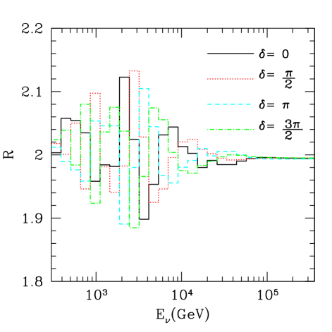
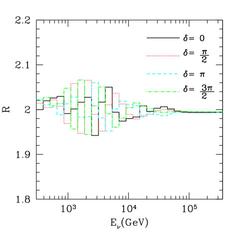
Figure 6: (Color online) The upper (lower) panel depicts the shower-to-muon track ratio for $\sin^{2}2\theta_{13}=0.15$, for Model [B], for the case of normal (inverted) hierarchy, for different values of the CP violating phase $\delta$.

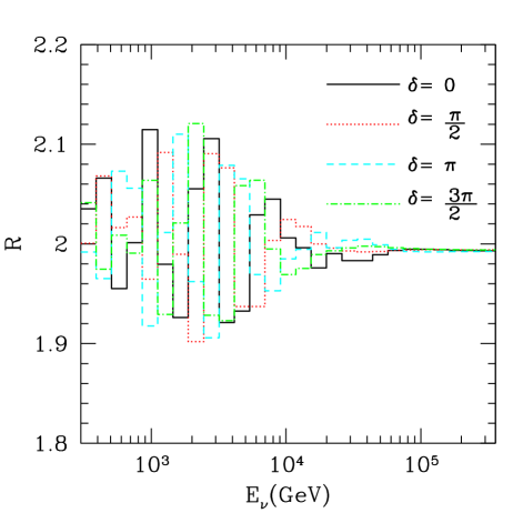
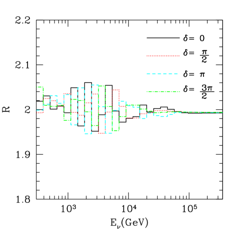
Figure 7: (Color online) The upper (lower) panel depicts the shower-to-muon track ratio for $\sin^{2}2\theta_{13}=0.15$, for Model [C], for the case of normal (inverted) hierarchy, for different values of the CP violating phase $\delta$.

Figures 6 and 7 depict the shower-to-muon track ratio for the density profiles given by the models [B] and [C] in Eqs. (2) and (3) respectively; and the previous discuussions on Model [A] in Fig. 5 apply to these cases as well.

A change in the dependence of the matter potential profile will affect the location of the energy at which the maximum matter effect is located. Depending on the specific form of the electron number density vs distance $N_{e}(r)$, a neutrino with a fixed energy $E_{\nu}$ will reach the resonant density at a different distance from the center of the astrophysical source, as can be seen from Fig. 8, where we have depicted the distance at which the resonant density is reached vs the neutrino energy $E_{\nu}$ for the three models. Notice that, for Model [C], there is a range of energies (between 100 and 500 GeV) for which the neutrino can profile, where the transition is highly non-adiabatic. The propagation inside the source from the production point to its surface is thus different measured spectral shape.

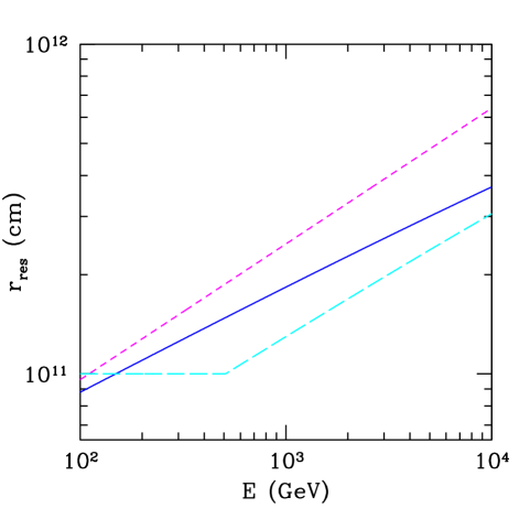
Figure 8: (Color online) Distance from the center of the astrophysical source (in cm), at which the resonant density is crossed vs the neutrino energy, for Model [A] (solid line), Model [B] (dashed line) and Model [C] (long-dashed line), for $\sin^{2}2\theta_{13}=0.15$.

It would be interesting to explore if it is possible to use neutrinos from astrophysical sources as those discussed here in order to explore neutrino properties like the neutrino mass ordering or the CP violating phase $\delta$.

A deviation from the expected $1:1:1$ ratio has been extensively explored in the literature (sometimes involving highly exotic scenarios), e.g., a different flavor ratio at the source rm ; Kashti:2005qa ; Kachelriess:2006fi , decaying neutrino scenarios bbhpw1 , Pseudo-Dirac schemes bbhlpw , additional sterile neutrinos Dutta:2001sf , magnetic moment transitions ekm and the possibility of measuring deviations from maximal atmospheric mixing serpico . An extensive discussion of possible deviations from the equal flavours scenario, including oscillations and decays beyond the idealized mixing case, characterization of the source and CPT violation was presented in bb . Some of these studies predict energy dependent ratios, however, none discussed matter effects on high-energy neutrino flux ratios as we explore in this paper.

If a relatively large deviation ($\sim 10\%$) of $R$ from its standard value $R\simeq 2$ is observed for energies $E<2$ TeV, one could infer a non zero value for the mixing angle $\theta_{13}$. The energy location of the matter enhanced peaks in the shower-to-muon track ratio depends on the precise value of $\theta_{13}$: for smaller values of $\sin^{2}2\theta_{13}<0.15$, the effect is larger (smaller) at lower (higher) energies with respect to the effect illustrated here for $\sin^{2}2\theta_{13}=0.15$, as expected from Eq. (25). Figure 9 shows the change in $R$ when varying $\theta_{13}$, for the Model A density profile, normal hierarchy and $\delta=0$. It can be seen that the results strongly depend on the $\theta_{13}$ mixing angle, whose effects get enhanced by a matter resonance for values larger than about $\sin^{2}2\theta_{13}=0.01$, when the transitions are mostly adiabatic.

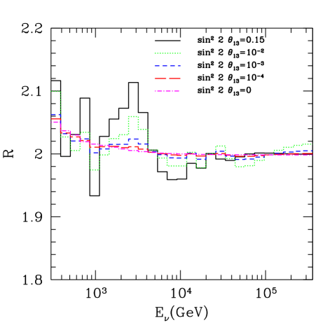
Figure 9: (Color online) Variation of $R$ with $\theta_{13}$.

Measuring the CP phase by observing the shower-to-muon track ratio is highly challenging, since for that purpose a precise knowledge of the matter density profile $\rho(r)$ would be required (see Ref. bbhpw2 for the prospects in a decaying neutrino scenario, Ref. Winter:2006ce for a combined analysis of neutrinos from reactors and optically thin astrophysical sources, and Ref. Costantini:2004ap ; Rodejohann:2006qq ; Fogli:2006jk ; Xing:2006uk for astrophysical neutrinos in different scenarios).

Under the assumption of a quite good knowledge of the density profile, it could be in principle possible to determine/verify the neutrino mass hierarchy since in all three models the effect is much higher in the normal mass ordering than in the inverted one regardless the value of the CP violating phase $\delta$. However, in practice, the errors on the remaining oscillation parameters might compromise the possibility of extracting the neutrino mass hierarchy, in particular the uncertainties on the atmospheric mixing angle $\theta_{23}$ (if a more precise knowledge of this mixing angle is not available at the time of the shower-to-muon track ratio measurement). Figure 10 shows the effects of changing $\theta_{23}$ between maximal mixing and $\sin^{2}\theta_{23}=0.38$ (the current 2 sigma allowed region), for the Model [A] density profile, normal hierarchy and $\delta=0$. Matter effects are, in general, larger for larger values of $\sin^{2}\theta_{23}$, except for very high energies when the ratios approach their values in vacuum. In this range, if $\theta_{23}$ is larger than $\pi/4$ the muon flux is enhanced and $R<2$, while the opposite is true if $\theta_{23}$ is smaller than $\pi/4$. The uncertainty in the mixing parameters would affect the possible determination of the mass hierarchy since the inverted hierarchy pattern could be confused with a smaller value of $\theta_{23}$. A separate measurement of electron and tau neutrinos would greatly improve this situation, allowing to extract both the hierarchy and the value of $\theta_{23}$.

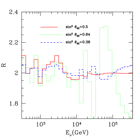
Figure 10: (Color online) Variation of $R$ with $\theta_{23}$.

VI Conclusions and outlook

We have discussed here high-energy neutrinos produced in optically thick (hidden) astrophysical objects for which large matter density inside the source can affect the oscillations of these neutrinos. The matter-induced transitions can lead to significant deviations from the 1:1:1 flavor ratios expected in standard scenarios. These deviations are expected at specific energies determined by the density profiles inside the sources. IceCube would be in an ideal position to measure such effects. The main observable that would be sensitive to these effects and that we have studied in detail is the shower-to-muon track ratio defined in Eq. (29).

A large number of events would be necessary in order to measure the effects of neutrino oscillations inside the source. In order to establish a 3 sigma effect, more than 1000 events would be needed. This would require a relatively nearby source, within a few megaparsecs. Given the supernova rate in nearby starburst galaxies such as M82 (3.2 Mpc) and NGC253 (2.5 Mpc) is about 0.1/yr, the possibility of such an event to take place is not rare assuming a significant fraction of SNe are endowed with jets  Razzaque:2004yv ; Ando:2005xi ; rmw05 . Upcoming neutrino telescopes will be able to constrain this fraction. The combined SN rate from all galaxies within 20 Mpc is more than 1/yr  Ando:2005ka .

With such large number of events it would also be possible, in principle, to investigate neutrino properties like the mass ordering and CP violating phase, especially if future reactor and accelerator experiments could provide a better measurement of the mixing angles. If all neutrino properties would already be known from other experiments, the shower-to-muon track ratio measured in IceCube could be used to determine source properties: matter effects inside the source reflected in the ratio $R$ are extremely sensitive to the source density profile.

Since high-energy $\gamma$-rays are not emitted from optically thick sources, it is hard to predict their occurrence rate. If a large population of hidden high-energy neutrino sources would exist in nature, then their combined effect would be evident in the ratio $R$ measured from diffuse fluxes. A modulation of $R$ with energy over a wide range is expected if the astrophysics varies from source to source and/or if the sources are distributed over a wide redshift. This is a distinct signal from the effect, e.g., discussed in Refs. rm ; Kashti:2005qa ; which appear only at ultrahigh-energies.

Neutrino telescopes are sensitive to the atmospheric neutrinos as well in the 0.1-100 TeV energy range we are interested in. However, the atmospheric neutrinos should not affect measurement of the ratio $R$ for a nearby transient point source that we are considering. For diffuse flux from all such point sources, the measured ratio will be a convolution of the atmospheric flux ratios and the astrophysical flux ratios. The oscillation effects for the atmospheric neutrinos is rather small ($<10\%$) because of a small $\Delta m^{2}L/E$. The experiments should be able to de-convolute them even without precise knowledge of the oscillation parameters. Assuming neutrino oscillation parameters are well-measured, matter oscillation effects as we discussed here would be the most natural explanation of any deviation of $R$ from its value in vacuum measured by upcoming neutrino telescopes.

References

- (1) See, e.g., C. D. Dermer, in the proceedings of 2nd Workshop on TeV Particle Astrophysics, Madison, Wisconsin, 28-31 Aug 2006. arXiv:astro-ph/0611191.
- (2) K. Hirata et al. [KAMIOKANDE-II Collaboration], Phys. Rev. Lett. 58, 1490 (1987).
- (3) G. M. Frichter, D. W. McKay and J. P. Ralston, Phys. Rev. Lett. 74, 1508 (1995) [Erratum-ibid. 77, 4107 (1996)] [arXiv:hep-ph/9409433].
- (4) R. Gandhi, C. Quigg, M. H. Reno and I. Sarcevic, Astropart. Phys. 5, 81 (1996) [arXiv:hep-ph/9512364].
- (5) R. Gandhi, C. Quigg, M. H. Reno and I. Sarcevic, Phys. Rev. D 58, 093009 (1998) [arXiv:hep-ph/9807264].
- (6) A. Achterberg et al. [IceCube Collaboration], Astropart. Phys. (in press) arXiv:astro-ph/0604450.
- (7) U. F. Katz, in the proceedings of 2nd VLVNT Workshop on Very Large Neutrino Telescope (VLVNT2), Catania, Italy, 8-11 Nov 2005. Nucl. Instrum. Meth. A 567, 457 (2006) [arXiv:astro-ph/0606068].
- (8) A. S. Dighe and A. Y. Smirnov, Phys. Rev. D 62, 033007 (2000) [arXiv:hep-ph/9907423].
- (9) W. Rodejohann, arXiv:hep-ph/0612047.
- (10) W. Winter, Phys. Rev. D 74, 033015 (2006) [arXiv:hep-ph/0604191].
- (11) P. D. Serpico and M. Kachelriess, Phys. Rev. Lett. 94, 211102 (2005) [arXiv:hep-ph/0502088].
- (12) P. D. Serpico, Phys. Rev. D 73, 047301 (2006) [arXiv:hep-ph/0511313];
- (13) M. L. Costantini and F. Vissani, Astropart. Phys. 23, 477 (2005) [arXiv:astro-ph/0411761].
- (14) Z. Z. Xing and S. Zhou, Phys. Rev. D 74, 013010 (2006) [arXiv:astro-ph/0603781].
- (15) M. Cirelli, N. Fornengo, T. Montaruli, I. Sokalski, A. Strumia and F. Vissani, Nucl. Phys. B 727, 99 (2005) [arXiv:hep-ph/0506298].
- (16) G. L. Fogli, E. Lisi, A. Mirizzi, D. Montanino and P. D. Serpico, Phys. Rev. D 74, 093004 (2006) [arXiv:hep-ph/0608321].
- (17) C. Lunardini and A. Y. Smirnov, Nucl. Phys. B 583, 260 (2000) [arXiv:hep-ph/0002152].
- (18) P. Mészáros and E. Waxman, Phys. Rev. Lett. 87, 171102 (2001) [arXiv:astro-ph/0103275].
- (19) S. Razzaque, P. Mészáros and E. Waxman, Phys. Rev. D 68, 083001 (2003) [arXiv:astro-ph/0303505].
- (20) S. Razzaque, P. Mészáros and E. Waxman, Phys. Rev. Lett. 93, 181101 (2004) [Erratum-ibid. 94, 109903 (2005)] [arXiv:astro-ph/0407064].
- (21) J. Alvarez-Muniz and P. Mészáros, Phys. Rev. D 70, 123001 (2004) [arXiv:astro-ph/0409034].
- (22) F. W. Stecker, Phys. Rev. D 72, 107301 (2005) [arXiv:astro-ph/0510537].
- (23) A.I. McFadyen, S.E. Woosley and A. Heger, Astrophys. J. bf 550, 410, 2001.
- (24) P. Mészáros and M.J. Rees, Astrophys. J. bf 556, L37, 2001.
- (25) E. Waxman and P. Mészáros Astrophys. J. bf 584, 390, 2003.
- (26) C.D. Matzner and C.F. McKee, Astrophys. J 510, 379 (1999)
- (27) R.A. Chevalier and N. Soker, Astrophys. J 341, 867 (1989)
- (28) S. Woosley, N. Langer and T. Weaver, Astrophys. J 411, 823 (1993)
- (29) T. Shigeyama and K. Nomoto, Astrophys. J 360, 242 (1990)
- (30) D. Arnett, Astrophys. J 383, 295 (1991)
- (31) S. Ando and J. F. Beacom, Phys. Rev. Lett. 95, 061103 (2005) [arXiv:astro-ph/0502521].
- (32) S. Razzaque, P. Mészáros and E. Waxman, Mod. Phys. Lett. A 20, 2351 (2005)
- (33) S. Eidelman et al., Phys. Lett. B 592, 1 (2004).
- (34) A. Cervera, A. Donini, M. B. Gavela, J. J. Gomez Cadenas, P. Hernandez, O. Mena and S. Rigolin, Nucl. Phys. B 579, 17 (2000) [Erratum-ibid. B 593, 731 (2001)] [arXiv:hep-ph/0002108].
- (35) M. Kachelriess and R. Tomas, Phys. Rev. D 64, 073002 (2001); G. L. Fogli, E. Lisi, D. Montanino and A. Palazzo, Phys. Rev. D 65, 073008 (2002), [Erratum-ibid. D 66, 039901 (2002)].
- (36) I. Mocioiu and R. Shrock, JHEP 0111, 050 (2001) [arXiv:hep-ph/0106139].
- (37) S. Ando, J. F. Beacom and H. Yuksel, Phys. Rev. Lett. 95, 171101 (2005) [arXiv:astro-ph/0503321].
- (38) J. P. Rachen and P. Mészáros, Phys. Rev. D 58, 123005 (1998) [arXiv:astro-ph/9802280].
- (39) T. Kashti and E. Waxman Phys. Rev. Lett. 95, 181101 (2005) [arXiv:astro-ph/0507599].
- (40) M. Kachelriess and R. Tomas, Phys. Rev. D 74, 063009 (2006) [arXiv:astro-ph/0606406].
- (41) J. F. Beacom, N. F. Bell, D. Hooper, S. Pakvasa and T. J. Weiler, Phys. Rev. Lett. 90, 181301 (2003) [arXiv:hep-ph/0211305].
- (42) G. Barenboim and C. Quigg, Phys. Rev. D 67, 073024 (2003) [arXiv:hep-ph/0301220].
- (43) J. F. Beacom, N. F. Bell, D. Hooper, J. G. Learned, S. Pakvasa and T. J. Weiler, Phys. Rev. Lett. 92, 011101 (2004) [arXiv:hep-ph/0307151].
- (44) S. I. Dutta, M. H. Reno and I. Sarcevic, Phys. Rev. D 64, 113015 (2001) [arXiv:hep-ph/0104275]; H. Nunokawa, O. L. G. Peres and R. Zukanovich Funchal, Phys. Lett. B 562, 279 (2003) [arXiv:hep-ph/0302039].
- (45) K. Enqvist, P. Keranen and J. Maalampi, Phys. Lett. B 438, 295 (1998) [arXiv:hep-ph/9806392].
- (46) J. F. Beacom, N. F. Bell, D. Hooper, S. Pakvasa and T. J. Weiler, Phys. Rev. D 69, 017303 (2004) [arXiv:hep-ph/0309267].