The VLA-COSMOS Survey:
II. Source Catalog of the Large Project

Abstract

The VLA-COSMOS large project is described and its scientific objective is discussed. We present a catalog of $\sim 3,600$ radio sources found in the $\rm 2\,deg^{2}$ COSMOS field at 1.4 GHz. The observations in the VLA A and C configuration resulted in a resolution of 1.5^′′$\times$1.4^′′ and a mean rms noise of $\rm\sim 10.5(15)\,\mu Jy/beam$ in the central $\rm 1(2)\,deg^{2}$. 80 radio sources are clearly extended consisting of multiple components, and most of them appear to be double-lobed radio galaxies. The astrometry of the catalog has been thoroughly tested and the uncertainty in the relative and absolute astrometry are 130 mas and $<$55 mas, respectively.

1 Introduction

The radio source counts above the milli-Jansky level are dominated by radio galaxies and quasars powered by active galactic nuclei (AGN) in elliptical host galaxies. However, deep radio surveys at 1.4 GHz show an upturn in the integrated source counts at sub-mJy levels revealing the presence of a population of faint radio sources far in excess of those expected from the high luminosity radio galaxies and quasars which dominate at higher fluxes (Windhorst et al., 1985; Hopkins et al., 1998; Ciliegi et al., 1999; Richards, 2000; Prandoni et al., 2001; Hopkins et al., 2003; Huynh et al., 2005). While radio sources with relatively bright optical counterparts are starburst galaxies (e.g. Benn et al., 1993; Afonso et al., 2005), the ones with fainter optical counterparts are often redder as expected for early type galaxies (Gruppioni et al., 1999). Recent detailed multi-wavelength follow-up of faint radio sources showed a mixture of active star forming galaxies and AGN hosts (Roche et al., 2002; Afonso et al., 2006). The exact mixture of these different populations (high-z AGN out to the highest redshifts, intermediate-z post starburst, and lower-z emission line galaxies) as a function of radio flux level is not very well established, especially in the $\mu$Jy regime.

In order to fully investigate the nature and evolution of the $\mu$Jy population it is necessary to couple deep radio observations with high quality imaging and spectroscopic data from other wavelengths covering as much of the electromagnetic spectrum as possible. The international COSMOS (Cosmic Evolution) survey (Scoville et al., 2006a) provides such a unique opportunity. COSMOS is a pan-chromatic imaging and spectroscopic survey of a $1.4^{\circ}\times 1.4^{\circ}$ field designed to probe galaxy and SMBH (super-massive black hole) evolution as a function of cosmic environment. One major aspect of the COSMOS survey is the HST Treasury project (Scoville et al., 2006b), entailing the largest ever allocation of HST telescope time. The equatorial location of the COSMOS field offers the critical advantage of allowing major observatories from both hemispheres to join forces in this endeavor. State-of-the-art imaging data at all wavelengths (X-ray to centimeter, e.g. Hasinger et al., 2006; Schiminovich et al., 2006a; Taniguchi et al., 2006; Capak et al., 2006; Bertoldi et al., 2006; Aguirre et al., 2006; Schinnerer et al., 2004) plus large optical spectroscopic campaigns using the VLT/VIMOS and the Magellan/IMACS instruments (Lilly et al., 2006; Impey et al., 2006; Trump et al., 2006) have been or are currently being obtained for the COSMOS field. These make the COSMOS field an excellent resource for observational cosmology and galaxy evolution in the important redshift range $z\sim 0.5-3$, a time span covering $\sim$75% of the lifetime of the universe.

One major scientific rationale of the COSMOS survey is to study the relation between the large scale structure (LSS) and the evolution of galaxies and SMBHs. In a $\Lambda$CDM cosmology, galaxies in the early universe grow through two major processes: dissipational collapse and merging of lower mass protogalactic and galactic components. Their intrinsic evolution is then driven by the conversion of primordial and interstellar gas into stars, with galactic merging and interactions triggering star formation and starbursts. Mergers also can perturb the gravitational potential in the vicinity of the black hole, thus initiating or enhancing AGN activity. Several lines of evidence suggest that galaxy evolution and black hole growth are closely connected; COSMOS offers the chance to observe this connection directly. While there is general agreement over this qualitative picture, the timing/occurrence of these events and their dependence on the local environment remains to be observationally explored (e.g. Ferguson et al., 2000). To study LSS it is essential to obtain high spatial resolution data over the entire electromagnetic spectrum covering a significant area on the sky, like 2 deg² as in the case of the COSMOS survey. Also, surveys of active galactic nuclei benefit from such a combination of areal coverage and depth.

For the radio observations at 1.4 GHz, it was essential to match the typical resolution for optical-NIR ground-based data of $\sim$ 1^′′ to fully exploit the COSMOS database. Therefore observations with the NRAO Very Large Array (VLA) had to be conducted in the A-array that provides a resolution of about 2^′′ (FWHM) at 1.4 GHz. Mosaicking is necessary to cover the large area of the COSMOS field. The VLA-COSMOS survey consists of the pilot project (Schinnerer et al., 2004), the large project (presented here) and the ongoing deep project (focusing on the central 1 deg²; Schinnerer et al., in prep.). The VLA-COSMOS pilot project tested the mosaicking capabilities in the VLA A-array at 1.4 GHz in the wide-field imaging mode and has provided the initial astrometric frame for the COSMOS field.

Here we present the source catalog derived from the 1.4 GHz image of the VLA-COSMOS large project. The paper is organized as follows: after a brief description of the survey objective (§2), the details of the observations and data reduction are presented in §3 and §4, respectively. In §5, we discuss our tests for flux and astrometric calibration. The VLA-COSMOS catalog is described in §6, while the context of the VLA-COSMOS survey within the COSMOS project is discussed in §7.

2 Survey Objective

Unlike most existing deep survey fields, the COSMOS field is equatorial and hence has excellent accessibility from all ground-based facilities (current and future such as [E]VLA and ALMA). In addition, it has an extensive multi-wavelength coverage (Scoville et al., 2006a). This makes it an ideal field to analyze the (faint) radio source population as a function of redshift, environment, galaxy morphology and other properties. The VLA-COSMOS radio observations were matched to study a range of important issues related to the history of star formation, the growth of super-massive black holes, and the spatial clustering of galaxies. The ongoing spectroscopic surveys within the COSMOS project are also targeting well-defined samples of radio sources as part of the overall program. In addition, the VLA-COSMOS radio survey is providing the absolute astrometric frame for the COSMOS field (Aussel et al., 2006), which is important given the field’s large size.

In this paper we describe in detail the observing procedure, and various tests on data quality and characteristics (astrometry, fitted source parameters, etc.; see also the pilot project paper by Schinnerer et al., 2004). The completeness tests and the number counts of this survey are under-way (Bondi et al., in prep.) as well as the identification of optical counterparts using the space- and ground-based COSMOS imaging data (Ciliegi et al., in prep.). The full source catalog is available from the COSMOS archive at IPAC/IRSA. Subsequent papers will consider important scientific issues such as: (i) the evolution of radio-loud AGN as a function of environment, including comparison to X-ray AGN and clusters (see also Smolčić et al., 2006), and a search for type-II radio QSOs, and (ii) a dust-unbiased survey of star forming galaxies, as revealed in the sub-mJy radio source population, including consideration of the evolution of the radio-FIR correlation out to $z\sim 1$ through comparison with the Spitzer data, and of extreme, high $z$ starbursts as seen in the MAMBO 250 GHz COSMOS survey (Bertoldi et al., 2006). In the following sections we describe the goals of these two key science programs in more detail.

2.1 Survey Area

The sub-mJy radio source counts provide one of the best indicators of the effect of cosmic variance: number counts of sub-mJy radio sources in fields of order of $\sim 10^{\prime}$ in diameter show a factor three variation (e.g. Hopkins et al., 2003), indicating that such field sizes are inadequate to map cosmic large scale structure. Thus to properly sample the faint radio source population and map out its cosmic structure to the largest relevant scales, it is necessary to survey a large area at the same resolution and sensitivity. Proper studies of source clustering require hundreds to thousands of sources. In order to enable detailed studies of environmental effects on faint, distant radio source distributions and properties, all as a function of redshift, several thousand sources are required as well.

Deep radio imaging of the $\rm 2\,deg^{2}$ COSMOS field with $\sim 3,600$ sources allows one to probe a - unique and - key area of parameter space. The combination of high sensitivity and high spatial resolution over a large area (see Tab. 1) bridges the gap between shallow, wider field surveys, such as FIRST (Becker et al., 1995) and NVSS (Condon et al., 1998) with about one million source entries, and ultra-sensitive ($\leq 5-7\mu$Jy), narrow field (single VLA primary beam $\sim 30^{\prime}$ FWHM) studies of a few hundred sources, such as those by Fomalont et al. (2006); Richards (2000). Surveys which are comparable in scope to the VLA-COSMOS large project are the Phoenix deep field survey (PDS), undertaken with the ATCA (Hopkins et al., 2003), and the VVDS 02hr field done with the VLA in B-array (Bondi et al., 2003). These surveys produce a lower angular resolution and a slightly higher rms (see Tab. 1).

2.2 Star Forming Galaxies

Tracing the evolution of the cosmic star formation history from optical surveys bears the large uncertainty of dust corrections (e.g Steidel et al., 1999). Deep VLA observations of the COSMOS field can provide a unique, unobscured look at star forming galaxies and highly extincted galaxies in the full range of environment, especially in combination with the deep (sub)mm data (Bertoldi et al., 2006; Aguirre et al., 2006) and deep Spitzer infrared imaging (Sanders et al., 2006) to which the high resolution of the VLA images provides means to properly identify luminous infrared galaxies (see Fig. 1). The VLA radio data will particularly be helpful to (a) trace the cosmological star formation history and (b) test the FIR/radio correlation at high redshifts. The radio luminosity of local galaxies is well-correlated with their star formation (SF) rate (Condon, 1992), and needs, unlike optical tracers, no correction for dust obscuration. Thus radio sources with correct spectral identification (as star forming galaxies) can be independently used to estimate the SF history (of the luminous sources).

Recent work by Haarsma et al. (2000) for three deep radio surveys confirms the trend of rising star formation rate between $z=0$ and $z=1$, however their calculated star formation rates are significantly larger than even dust-corrected optically selected star formation rates. A key uncertainty is the contribution of AGN to the faint ($\rm<1mJy$) radio population, with estimates ranging from 20$\%$ to 80$\%$ for surveys down to 40 $\mu$Jy. The (far)IR-radio correlation for star forming galaxies appears to hold out to high redshift (Garrett, 2002; Appleton et al., 2004). However, the number of star forming sources detected at 1.4 GHz is small above $z=0.5$. A thorough understanding of the IR-radio correlation out to higher redshifts is important, as it has been widely used as a distance measure for sub-mm sources without any optical counterparts (Carilli & Yun, 2000; Aretxaga et al., 2005). Also, an important question for active star forming galaxies is the role of mergers, in particular at higher redshift. The FIR imaging alone will lack sufficient resolution to address this issue, while the optical imaging will suffer from the standard problem of obscuration in these very dusty systems. Only arcsecond resolution radio data will allow the determination of the spatial distribution of star formation in dusty starbursts on scales relevant for merging galaxies ($\sim 10$ kpc).

2.3 Active Galactic Nuclei

Only a large field and deep radio survey can provide information about the evolution of the currently highly uncertain faint-end of the radio luminosity function. The fundamental problem in the study of the evolution of radio-loud AGN has been that samples are drawn from either very wide field, but very shallow surveys, or very deep, but very small field surveys. The former are limited at high redshifts to only extreme luminosity sources, while the latter are plagued by relatively small number statistics and number variance. The VLA-COSMOS survey was designed to enable the study of the demographics and evolution of AGN by encompassing a large cosmological volume and by providing good statistics on both radio-loud and radio-quiet AGN as a function of redshift.

Only sub-mJy sensitivities over a wide area are adequate to detect relatively weak (FRI) radio AGN to very high redshift ($\rm z\sim 6$) while providing a large number ($\sim 1000$) of AGN sources. At lower redshift, z $\sim$ 1, a sensitivity of $\rm 1\sigma\approx 10\,\mu Jy/beam$ is good enough to detect a significant fraction of radio-quiet, optically-selected QSOs. Moreover, questions regarding redshift evolution of FRI and FRII sources, their parent galaxy properties, and environmental dependencies can be addressed independently for QSOs and radio galaxies. Such observations are sensitive enough to reach the classic boundary between radio-loud and radio-quiet AGN (log L${}_{1.4\,\rm{GHz}}\,[\mathrm{W\,Hz}^{-1}]$ = 25) at z $\sim$ 4-5 (depending on the exact spectral index; see Fig. 1). Highly luminous radio-loud objects such as Cygnus A with log L${}_{1.4\,\rm{GHz}}\,[W\,Hz^{-1}]\sim$ 34 (Carilli & Barthel, 1996) should be observable out to their epoch of formation.

3 Observations

The goal of the large project of the VLA-COSMOS survey was to image the entire COSMOS field with an as large as possible uniform rms coverage while minimizing the observing time required. Since the observations had to be finished within one configuration cycle, special requirements arose for the pointing lay-out and the observing strategy.

3.1 Lay-out of the Pointing Centers

The pointing lay-out was designed to maximize the uniform noise coverage while minimizing the number of pointings required to limit overhead due to slewing ($\sim$30 s slewing time for each change of pointing). A hexagonal pattern of the pointing centers provides both a uniform sensitivity distribution and a high mapping efficiency for large areas (see Condon et al., 1998). To minimize the effect of bandwidth smearing, we used – as already tested in the pilot observations (Schinnerer et al., 2004) – a separation of $15^{\prime}$ between the individual field centers. A total of 23 separate pointings was required to fully cover the $\rm 2\,deg^{2}$ of the COSMOS field (see Tab. 2 and Fig. 2).

3.2 Correlator Set-up and Calibrators

We used the standard VLA L-band continuum frequencies of 1.3649 and 1.4351 GHz and the multi-channel continuum mode to minimize the effect of bandwidth smearing (in the A configuration). This results in two intermediate frequencies (IF) with two polarizations, providing 6 useable channels of 3.125 MHz each, or a total bandwidth of 37.5 MHz (observed with both polarizations). (Nominally, 7 channels are available, however, due to the largely reduced sensitivity in the last channel, we only used channels 1 to 6.)

The quasar 0521+166 (3C 138) served as flux and bandpass calibrator and was observed at the beginning of each observation. To allow for good correction of atmospheric amplitude and phase variations, we selected the quasar 1024-008 which was already used in the pilot observations (Schinnerer et al., 2004). 1024-008 is about 6.1^∘ away from the COSMOS field center and has a flux of about 1 Jy at 1.4 GHz. Its positional accuracy is better than $0.01^{\prime\prime}$ (VLA Calibrator Manual 2003); the positional difference is less than $0.001^{\prime\prime}$ between coordinates listed in the VLA Calibrator Manual and its ICRF (International Celestial Reference Frame; Fey et al., 2004) position.

The quasar 0925+003 at a distance of about 9^∘ from the COSMOS field center was observed to test the absolute astrometric accuracy of the observations. Its positional accuracy is known to better than $0.002^{\prime\prime}$, and its 1.4 GHz flux is similar to the one of 1024-008. It was also used to test the flux calibration (see Section 5).

3.3 Observing Strategy

This project holds the status of a VLA Large Project, as it required 240 hrs of observing time in the A configuration alone. The observations were scheduled in blocks of 6 hrs centered at the Local Siderial Time (LST) of 10:00 hr. This ensured that the COSMOS field was always above 40^∘ elevation during our observations to keep the system temperature of the L-band receivers low. These observing blocks were scheduled over 42 days between September 23th, 2004 and January 9th, 2005 for the A configuration, and between August 26th, 2005 and September, 25, 2005 for the C configuration. The observing time for the C configuration consisted of 4 observing blocks each 6 hrs long, except for the last observation that was 1.5 hrs longer.

In order to minimize the impact of varying observing conditions – especially during the A array observations – onto the mosaic we adopted the following scheme: (a) all 23 pointings were observed with about 6.5 minutes integration time twice each day, (b) the starting pointing was changed each time, (c) the flux calibrator 0521+166 was only observed at the beginning (since interpolation between days in case of a loss was acceptable (d) the phase calibrator 1024-008 was observed every 28 to 35 minutes, and (e) the test calibrator 0925+003 was observed twice each day after about one-third and two-thirds of the available observing time. The rotation of the pointings with observing days also resulted in a more complete $uv$ coverage, and therefore a rounder synthesized (i.e. DIRTY) beam.

4 Data Reduction and Imaging

4.1 Data Reduction

The data reduction was done using the Astronomical Imaging Processing System (AIPS; Greisen, 2003) following the standard routines as described in the VLA handbook on Data Reduction. For the flux calibration and the correction of the atmospheric distortions we used the pseudo-continuum channel. Before and after this calibration, $uv$ points (of the two calibrators 0521+166 and 1024-008) affected by radio frequency interference (RFI) were flagged by hand using the AIPS task ’TVFLAG’. As the data were obtained in the multi-channel continuum mode, a bandpass calibration was performed on the ’Line’ data after the flux and phase calibration of the pseudo-continuum channel had been transfered to the ’Line’ data. In order to exclude remaining RFI in the source data (i.e. the individual COSMOS fields), we checked all channels (per IF and polarization) for RFI using ’TVFLG’ and flagged affected points accordingly. During all A-array observations, significant RFI (affecting $\sim$ 15% of the data) was found to be present on IF2 in channel 4 to 6. In addition, all $uv$ data points in the A-array data above an amplitude of 0.4 Jy were clipped, since no such strong source is present in any individual field. The C-array observations were affected by strong RFI and solar interference, so that only baselines larger than 2.5 k$\lambda$ and 1 k$\lambda$ were included from the data of the first three days and the last day of observations, respectively. The clipping level was set to 0.45 Jy for the C-array data.

4.2 Imaging

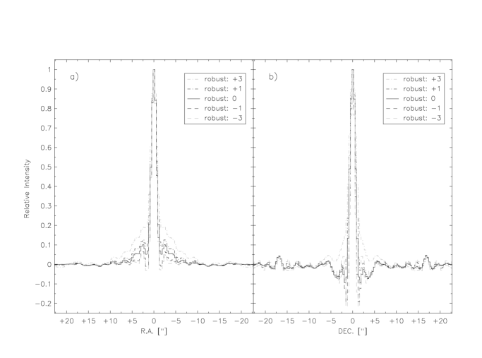
Figure 3: Cuts along the x- (a) and y-axis (b) of the synthesized (i.e. DIRTY) beam for different values of the robust weighting: +3 (grey dashed dotted line), +1 (dashed dotted line), 0 (solid line), -1 (dashed line), and -3 (grey dashed line). A value of 0 for the robust parameter gave the best compromise between synthesized beam shape and rms noise (see text for details).

We performed substantial testing for best imaging quality including the application of self-calibration on the COSMOS fields themselves. It was found that no combination of parameters for the self-calibration in the task ’CALIB’ would yield a significant improvement of the rms (of $>$ 3%). A robust weighting of 0 provided the best compromise for the combined A+C array data between a fairly Gaussian synthesized beam (Fig. 3), and still good sensitivity, i.e. the deviation from Gaussianity only starts below $\pm$10% of the peak. This proved to be especially important for fields which contained bright sources (with peak fluxes up to 10 mJy/beam) where tests showed that sidelobe artifacts are lowest when using a robust weighting of 0. The nominal increase in the noise compared to natural weighting is 1.265. However, the gain in better cleaning results around bright sources is larger than this nominal increase. Thus in order to achieve an uniform as possible rms across the entire COSMOS field, a robust weighting of 0 is used.

In order to avoid geometric distortions due to the non-planarity of the wide-field on the sky, each field was divided into 43 facets of 2048$\times$2048 pixels which were imaged using the option DO3DIMAG in the AIPS task ’IMAGR’. The pixel scale of $0.35^{\prime\prime}$/pixel has been well matched to the A+C-array beam size of FHWM $1.5^{\prime\prime}\times 1.4^{\prime\prime}$ (PA $\sim-50^{o}$) for a robust weighting of 0 (Fig. 3 and 4). For each field, a contiguous area of about 1^∘ diameter was covered by the facets. Additional smaller facets of 128$\times$128 pixels were made using the task ’SETFC’ for positions of NVSS sources with peak fluxes above 0.1 Jy and within a radial distance of 1.5^∘ from the pointing center. This ensured that sidelobes from strong sources outside the central 1^∘ were CLEANed as well.

Since most of the COSMOS fields are affected by the sidelobes of radio galaxies with peak fluxes between 1 to 15 mJy/beam, best CLEANing results were obtained if CLEAN boxes for individual sources were provided. This ensured that CLEANing of negative or positive residuals was minimized. In order to derive the CLEAN boxes for each field, we used the AIPS task ’IMAGR’ to interactively select the CLEAN boxes in all facets where significant sources were present. This procedure was performed combining the data of all polarizations and IFs into one single image to obtain the highest possible S/N image. The resulting list of CLEAN boxes was saved. In addition, we required that CLEAN components were subtracted from the $uv$ data after a facet had been cleaned. This way, CLEAN components in overlapping facets were not treated separately. In addition, this requirement also reduced the effect of sidelobe bumps from strong sources in neighboring facets.

We would like to note at this point that the reduction process of the VLA-COSMOS Pilot and Large dataset was not exactly identical. While self-calibration was applied to the Pilot data, this step was not done while reducing the Large survey data: after detailed empirical testing of the improvements due to self-calibration in the VLA-COSMOS Large project, we concluded that no significant improvement was achieved, likely due to the lack of sufficiently bright sources in all parts of the entire COSMOS field. Since self-calibration adjusts the observed visibility phases to model phases, it has the potential to alter the position of a given source. However, it is expected that these effects cancel out when using several sources within a given pointing.

For the final stage of CLEANing, it turned out that the well known ’beam squint’ of the VLA (i.e. slightly different pointing centers for R and L polarization), and the slightly different frequency coverages required separate imaging of all polarizations and IF combinations. The four separate ’IMAGR’ runs were performed with the same list of CLEAN boxes in the automatic mode. The number of iterations was set to 100,000, with a flux limit of 45 $\mu$Jy/beam ($\sim 1.5\sigma$ in a single image of a field) and a gain of 0.1 to optimize the CLEANing of the facets. The 43 facets forming the contiguous area were combined using the AIPS task ’FLATN’. The four separate images were then combined using the AIPS task ’COMB’ to obtain a single image for each field. Due to the combination of bandwidth smearing and a significant drop in sensitivity outside the radius of the Half Power Beam Width, we decided to use a cut-off radius of 0.4 (corresponding to a radius of $16.8^{\prime}$) when combining the individual fields into the final mosaic using the task ’FLATN’. The resulting image is shown in Fig. 5.

5 Tests

We performed a number of tests to evaluate our flux (see §5.1) and astrometric calibration (see §5.2) as well as the impact of the CLEAN procedure. For the last point, we performed a Gaussianity test on the noise. The noise was extracted from a roughly $16^{\prime}\times 11^{\prime}$ box close to the COSMOS field center. The individual noise pixels show a Gaussian distribution (Fig. 6). A Gaussian fit gives an rms of $\rm 10.09\,\mu Jy/beam$ ($\sigma$) (corresponding to a FWHM of $\rm 23.76\,\mu Jy/beam$). All noise distributions extracted for various boxes across the part of the field that has an uniform background showed a Gaussian distribution demonstrating that no artifacts have been introduced during the CLEAN process.

5.1 Flux calibration

The second phase calibrator 0925+003 was observed twice each day to allow for assessment of the absolute astrometry and the flux calibration. Most of the following tests were performed on the A-array only data, since it covered a wide range in time. We imaged the calibrator 0925+003 for each day, as well as the two observations per day separately. All IFs were combined at once, since the source of interest is at the phase center and any effects due to misalignment should be negligible. The images were cleaned with $1000$ iterations. The resulting typical resolution and rms were $1.96^{\prime\prime}\times 1.60^{\prime\prime}$ (FWHM) and $\sim 870\,\mu$Jy/beam, respectively. The position and flux of 0925+003 were derived by Gaussian fitting using the AIPS task ’JMFIT’ on the individual images.

For most of the days 0521+166 served as the flux calibrator. The trends of the peak flux of 0925+003 and 1024-008 are not the same over the course of the observations in the A configuration (Fig. 7) indicating no systematic effects in the flux calibration. Note that the error in the flux estimation for calibrator 1024-008 is significantly higher on day MJD 60038 (November 11th, 2004). This is due to strong interferences that could not be entirely removed in the $uv$ data points.

We compared the peak flux density values of 0925+003 of the two observations per day (Fig. 8). The median offset is 4.5 mJy/beam which corresponds to less than $1\%$ of the total flux density of 0925+003. The outliers correspond to days MJD 59990 (September 24th, 2004), 60011 (October 15th, 2004) and 60096 (January 8th, 2005). The rms in the maps for those days is about $1.3-2.6$ times the typical rms in the 0925+003 maps. The higher noise is likely to be caused by worse weather conditions (e.g. it was snowing on November 13th, 2004) and/or technical problems during observations (e.g. RFI, intermittent fluctuations of the system temperature $T_{SYS}$, data corruption on particular antennas). Thus we conclude that our flux calibration is within the errors expected.

5.2 Absolute and Relative Astrometry

Given the angular resolution of the combined A+C array data of $1.5^{\prime\prime}\times 1.4^{\prime\prime}$ (FWHM), we expect to achieve a positional accuracy of $\sim 0.15^{\prime\prime}$ (corresponding to 1/10th of the beam size; see Fomalont, 1999) for high S/N sources and $\sim\rm\frac{FHWM}{S/N}$ for lower S/N cases when extracting the source position within the COSMOS field.

In order to assess the quality of the absolute astrometric calibration, all observations of 0925+003 were combined into a single image. A non-zero offset in RA and DEC of 53 mas and 45 mas, respectively, has been found relative to the nominal position of 0925+003. This offset is likely the result of the large angular separation of 14.5^∘ between the two calibrators (i.e. 0925+003 and 1024-008), which could lead to residual phase transfer errors due to, for example, differential refraction corrections. We consider this offset as an upper limit to our absolute astrometry error, since the (center of the) COSMOS field is only 6^∘ away from the phase calibrator 1024-008.

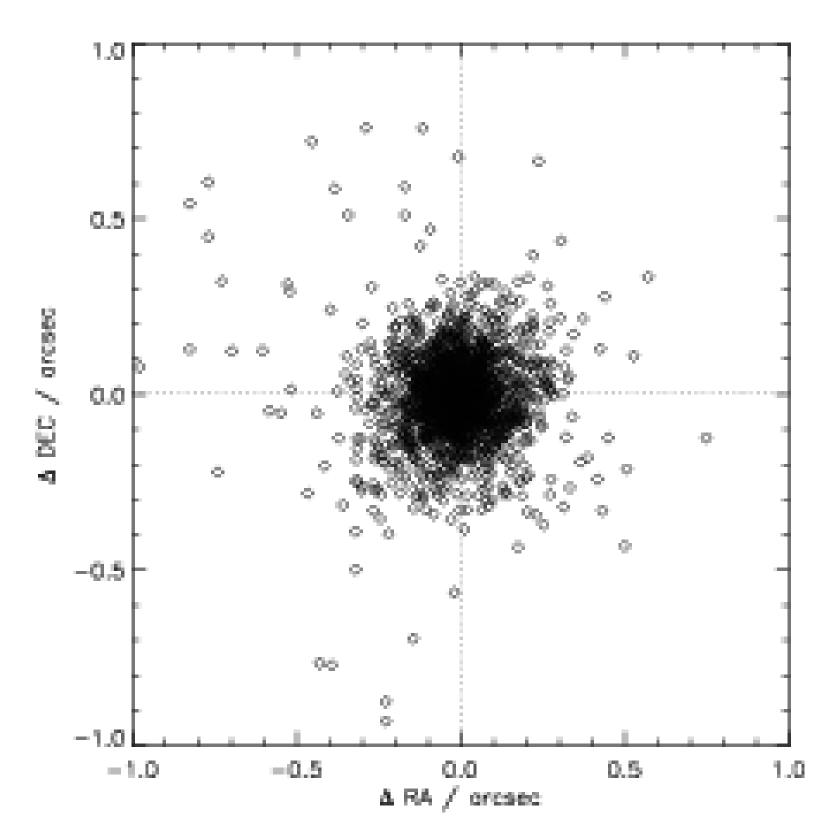
Figure 9: The left panel compares the offset in RA ($\Delta RA$) with the offset in DEC ($\Delta DEC$) when positions in single pointings are matched to positions in the combined mosaic (see text for details). The reference position is the one extracted from the mosaic. The right panel shows the distributions of $\Delta RA$ (thick dashed line) and $\Delta DEC$ (thin solid line). The total number of sources, mean and standard deviation of the offsets are indicated.

To test the quality of our relative astrometry, we extracted sources from each single field and compared their positions to the ones extracted from the combined mosaic. We searched for sources using the AIPS task ’SAD’ (Search And Destroy). On single fields we ran ’SAD’ searching for sources with fluxes higher than 100 $\mu$Jy/beam. ’SAD’ looks for points above the specified flux limit and merges such points into contiguous “islands”. Then it fits components within these “islands”. For our astrometric tests, we run ’SAD’ rejecting components within an island with both peak and integrated flux values lower than 100 $\mu$Jy/beam which corresponds to $\sim 7\sigma$ in a single field. On average $\sim 150$ sources were found per pointing. (In §6 we describe how ’SAD’ was run on the mosaic.) After source extraction we only matched positions of objects which have a deconvolved major axis of $<3^{\prime\prime}$ FWHM and are within a radius of $\sim 17^{\prime}$ from the pointing center (which corresponds to our primary beam cut of 0.4) in the specific field. We analyzed the offsets in right ascension ($\rm\Delta\,RA$) and declination ($\rm\Delta\,DEC$) in the central $\rm 0.87\,deg^{2}$ where the rms noise is basically uniform. The results are shown in Fig. 9. The offsets in $\rm\Delta\,RA$ and $\rm\Delta\,DEC$ are $(-10\pm 127)$ mas and $(-12\pm 131)$ mas, respectively. To search for possible systematic effects, we analyzed the $\Delta RA$ and $\Delta DEC$ offsets in different parts of the central $\rm 0.87\,deg^{2}$ area. As seen from Fig. 10, there are no significant systematic effects in our relative astrometry as a function of position within the COSMOS field.

To get a deeper insight into our astrometry we cross-correlated the COSMOS mosaic source catalog with the VLA FIRST survey catalog (Becker et al., 1995). To minimize the number of spurious matches, we used a search box size of $2^{\prime\prime}$ on a side. Only sources with a major axis $<3^{\prime\prime}$ and COSMOS to FIRST fluxes comparable within 20%, i.e. $\rm 0.8<S^{int}_{COSMOS}/S^{int}_{FIRST}<1.2$, were compared. Multiple component sources and FIRST sources with side lobe flags ($flag=1$) were excluded. Our final sample of matched sources contains only $28$ objects. The mean offsets and the $1\sigma$ errors for $\rm\Delta RA=RA_{COSMOS}-RA_{FIRST}$ and $\rm\Delta DEC=DEC_{COSMOS}-DEC_{FIRST}$ are $(-110\pm 273)$ mas and $(67\pm 232)$ mas, respectively. Given the low number of matched sources and the FIRST survey’s astrometric accuracy of 500 mas (or more) for individual sources (White et al., 1997), we conclude that the inferred positional offsets are within the source extraction errors of both surveys.

In addition, we compared the positions of radio sources extracted from the VLA-COSMOS Pilot and the Large project. However, we consider this not a completely independent test, as the same phase calibrator was used for both projects. We find a median offset of -50 mas and 90 mas in $\rm\Delta RA$ and $\rm\Delta DEC$, respectively, while the rms scatter is 161 mas and 189 mas for the first and latter. The rms scatter is slightly higher than the above derived accuracy of our relative astrometry ($\sim$130 mas) using only the Large project. However, this is expected as the rms and the beam size of the Pilot project is larger: 25 $\mu$Jy/beam vs. 10 $\mu$Jy/beam and $1.9^{\prime\prime}\times 1.6^{\prime\prime}$ vs. $1.5^{\prime\prime}\times 1.4^{\prime\prime}$. The derived astrometric differences between the Pilot and the Large projects are well within our errors (see §4.2 for data reduction difference between both projects). Hence, we conclude that our relative astrometric accuracy for the VLA-COSMOS Large project is $\sim$130 mas and discard this higher rms scatter found from the comparison to the Pilot data.

Based on arguments presented above, we conclude that the overall astrometric errors of our derived source positions are dominated by the uncertainty in the position extraction (due to our beam size) of $\sim 130$ mas. Our absolute astrometric accuracy is likely to be better than 55 mas.

6 The VLA-COSMOS Catalog

6.1 Source Extraction

In order to select a sample of radio components from the largest imaged area above a given threshold, defined in terms of the local signal to noise ratio, we adopted the following approach. First the software package SExtractor was used to estimate the local background in each mesh of a grid covering the whole surveyed area (see Bertin & Arnouts, 1996, for a general description of SExtractor). Different noise maps with mesh sizes ranging from 25 to 100 pixels were produced and examined. The fractional difference between the rms measured in the SExtractor noise maps and the rms directly measured on the real map is very small ($\sim$2%) over the whole map (see Fig. 11). In the end, we adopted a mesh size of 50 pixels corresponding to $17.5^{\prime\prime}$ which was found to be the best compromise between closely sampling the variations in rms and avoiding contamination by larger radio sources. The rms values range from about 9 $\mu$Jy/beam in the inner regions to about 20 $\mu$Jy/beam at the edges of the mosaic with values as high as $30-40\,\mu$Jy/beam around the few relatively strong sources (see Fig. 12). The mean rms in the inner $\rm 1\,deg^{2}$ is 10.5 $\mu$Jy/beam, the mean rms over the $\rm 2\,deg^{2}$ area is 15.0 $\mu$Jy/beam. The cumulative area as a function of rms is shown in Fig. 13.

As a next step, the AIPS task ’SAD’ was used to obtain a catalog of candidate components. ’SAD’ attempts to find all the components whose peaks are brighter than a given flux level. In order to detect radio components down to the 30 $\mu$Jy/beam level ’SAD’ was run several times with different search levels (with a decreasing flux limit) using the resulting residual image each time. We recovered all the radio components with a peak flux $\rm S_{peak}>30\,\mu Jy/beam$ (corresponding to roughly 3$\sigma$ in the higher sensitivity regions). For each component ’SAD’ provides peak flux, total flux, position and size estimated using a Gaussian fit.

However, for faint components the Gaussian fit may be unreliable and a better estimate of the peak flux (crucial for the selection based on S/N) can be obtained with a non-parametric second-degree interpolation using the AIPS task ’MAXFIT’. We ran ’MAXFIT’ on all the components found by ’SAD’ and selected only those components for which the peak flux density found by ’MAXFIT’ was greater or equal to 4.5 times the local rms as derived from the noise map. The (non-parametric) peak position and flux density as determined by ’MAXFIT’ were kept, as the so derived values should be less affected by assumptions on the real brightness distribution.

Finally, we visually inspected the S/N mosaic image (Fig. 14) for components that could have been missed by ’SAD’. The most likely reason for missing sources is that ’SAD’ only recovers components that can be fitted by a Gaussian fulfilling certain parameters. Thus, if the fit for a potential component fails, this component is rejected from the catalogue provided by ’SAD’. Therefore, the AIPS tasks ’JMFIT’ and ’MAXFIT’ were run on these potential components to derive their properties.

In order to exclude 1-pixel wide noise peaks above the detection threshold (4.5$\sigma$), more scrutiny was used for the 294 components fitted with both sizes smaller than the CLEAN beam. Only those components (171) for which JMFIT was able to estimate an upper limit to the source size greater than the CLEAN beam were kept while the remaining (123) were identified as noise spikes and excluded from the catalogue. As a result of the whole procedure a total of 3823 components have been selected (3204 from ’SAD’+’MAXFIT’ and 619 from the S/N image). A more complete analysis on the completeness and possible biases affecting the catalogue will be described in a future paper along with the number counts (Bondi et al., in prep).

6.2 Description of the Catalog

Some of the components clearly belong to a single radio source (e.g. jets and lobes of an extended radio galaxy), in other more complex cases we have also used the optical ground- and space-based images to discriminate between different components of the same radio source or separate radio sources. The final catalog (see Tab. 3; see below) lists 3643 radio sources of which 80 are multiple, i.e. better described by more than a single component. These sources are identified by the flag ’mult=1’ (Tab. 3). For these sources, the listed center is either the one of the radio core or the optical counterpart when either of these could be reasonably identified or the luminosity weighted mean position. In addition, we visually inspected weak ($\leq 6\sigma$) sources close to bright sources with significant sidelobes. A total of 72 sources potentially lying on sidelobe spikes are flagged with ’slob=1’.

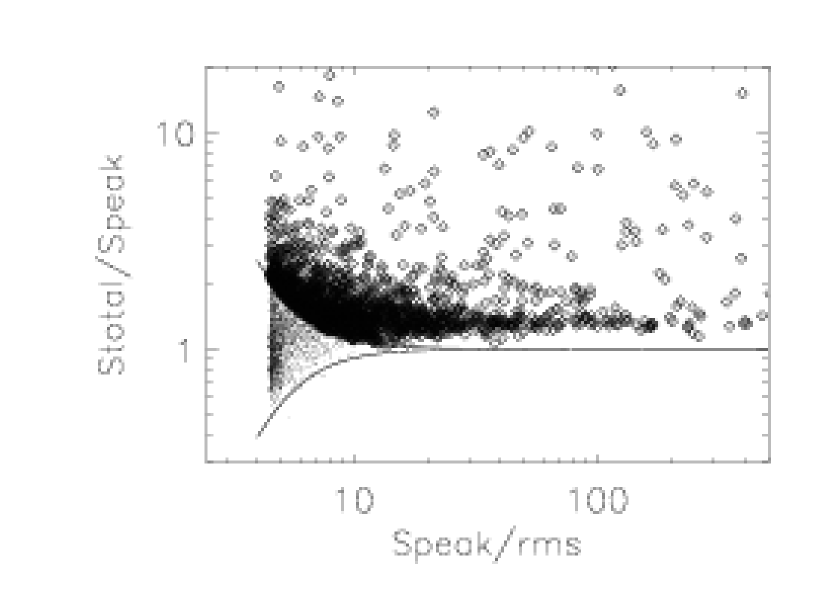
Figure 15: Ratio of the total flux $S_{T}$ to the peak flux $S_{P}$ as a function of the signal-to-noise ratio of the peak flux and the local rms. The solid line shows the upper and lower envelopes of the flux ratio distribution containing the sources considered unresolved (see text). Open symbols show sources considered resolved.

In Fig. 15 we plot the ratio of the total integrated flux density $S_{total}$ and the peak flux density $\rm S_{peak}$ as functions of the signal to noise ratio S/N ($\rm S_{peak}/rms$) for all the 3643 sources in the catalog. To select the resolved sources, we determined the lower envelope of the points in Fig. 15 which contains 99% of the sources with $S_{total}<S_{peak}$, and mirrored it above the $S_{total}/S_{peak}=1$ line (upper envelope in Fig. 15). We have considered the 1601 (44%) sources laying above the upper envelope resolved. The envelope can be described by the equation

$$\rm S_{total}/S_{peak}=1+[100/(S_{peak}/rms)^{3}]$$

The resolved sources are flagged in the catalog by ’res=1’. For the unresolved sources the total flux density is set equal to the peak brightness and the angular size is undetermined.

We calculated the uncertainties in the peak flux density $S_{peak}$ and integrated flux $S_{total}$ using the equations given by Condon (1997) as outlined in e.g. Hopkins et al. (2003); Schinnerer et al. (2004). For the positional uncertainties we used the equations reported in (Bondi et al., 2003, their equations 4 and 5), using 130 mas as the calibration error in right ascension and declination (see also Condon et al., 1998, their equation 27).

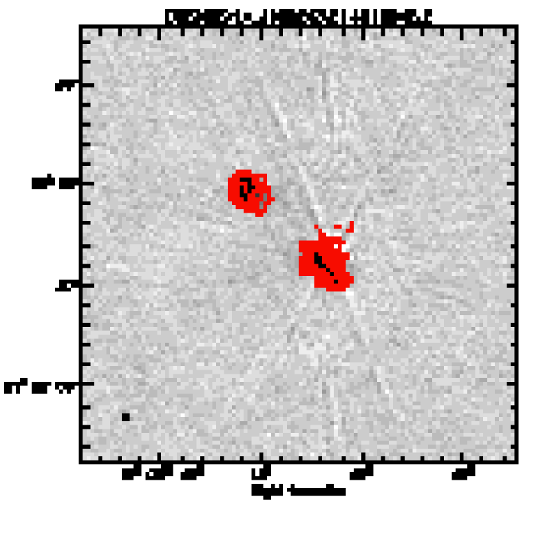
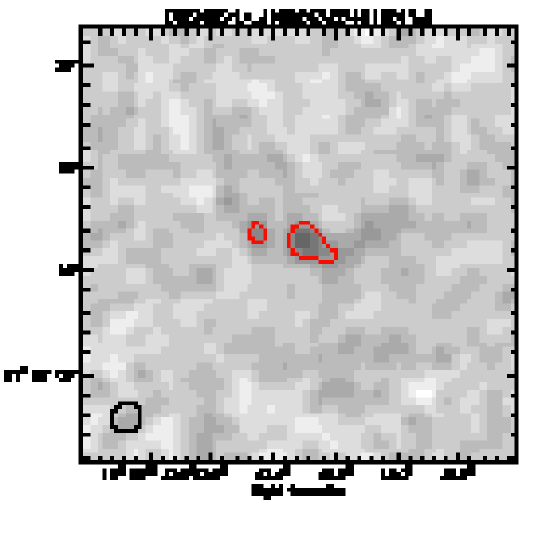
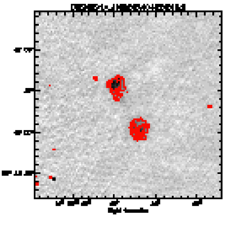
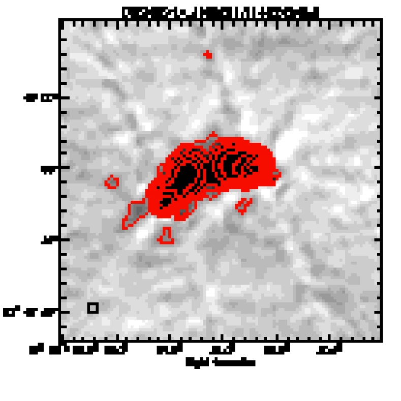
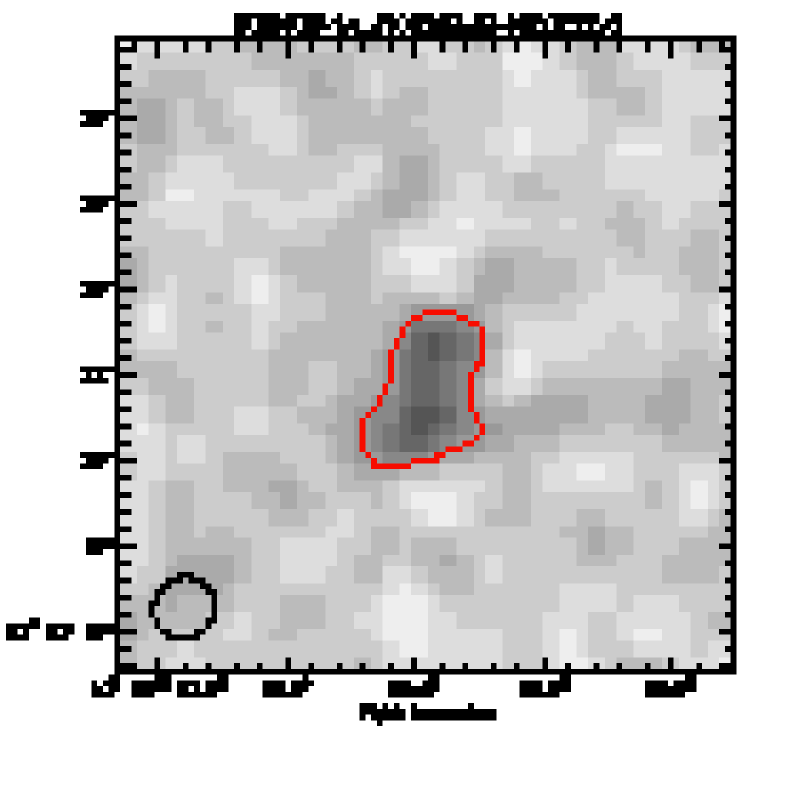
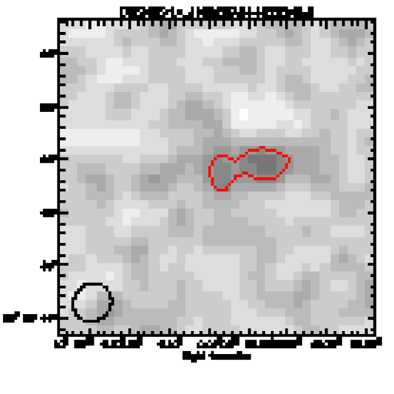
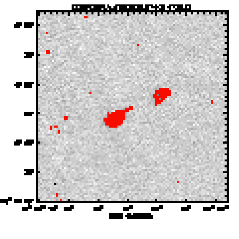
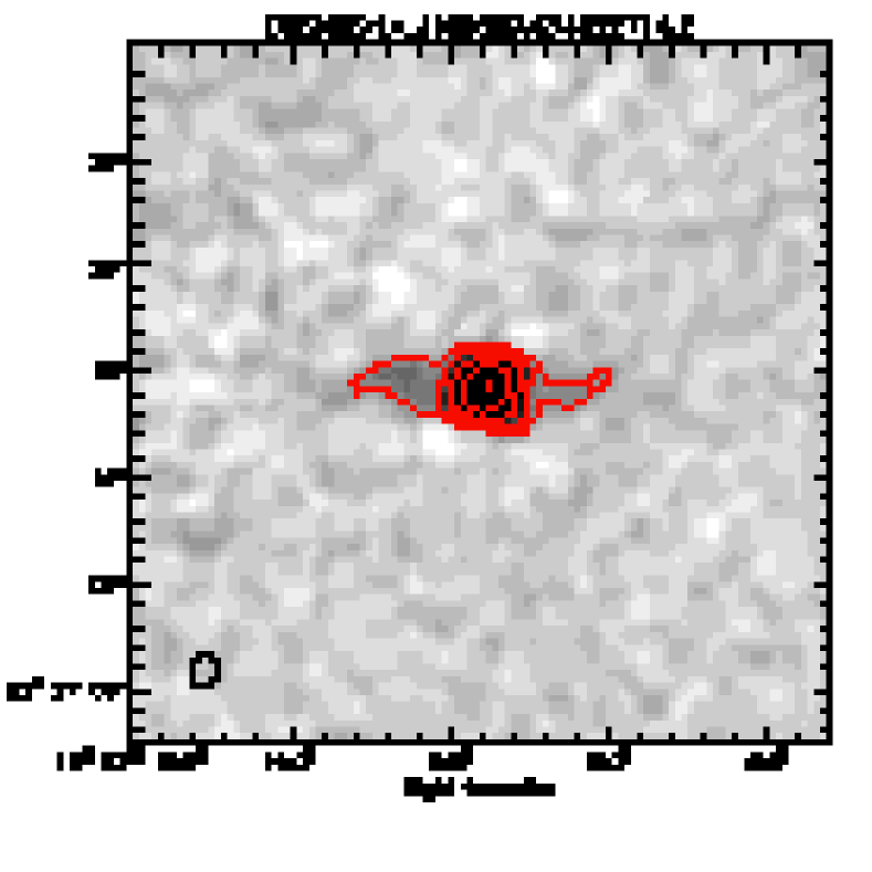
Figure 16: Radio sources fitted by multiple Gaussian components and identified as a radio group (see Tab. 4). The source name is given at the top of the individual panels. The grey-scale is from -4$\sigma$ to 10$\sigma$ of the local rms (Tab. 3). The contours start at 4$\sigma$ in steps of $2^{n}\times\sigma$ with $n=2,3,4,5,\dots$. (The local rms is listed in Tab. 3.) The beam is shown for reference in the bottom left corner.

For each of the 80 sources fitted with multiple components (see Fig. 16) we list in the multiple source catalog (see Tab. 4) (i) an entry for each of the components identified with a trailing letter (A, B, C, …) in the source name (from Tab. 3), and (ii) an entry for the whole source as it is listed in the source table (Tab. 3). In these cases the total flux was calculated using the task ’TVSTAT’, which allows the integration of map values over irregular areas, and the sizes are the largest angular sizes. For these sources the peak flux (at the listed position) is undetermined and therefore set to a value of ’-99.999’.

For each source we list the source name as well as its derived properties and their uncertainties. All 3643 radio sources are listed in right ascension order in Tab. 3 with the following columns:

Column(1): Source name
Column(2): Right ascension (J2000.0)
Column(3): Declination (J2000.0)
Column(4): rms uncertainty in right ascension
Column(5): rms uncertainty in declination
Column(3): Peak flux density and its rms uncertainty
Column(4): Integrated flux density and its rms uncertainty
Column(5): rms measured in the SExtractor noise map
Column(9): Deconvolved source size – major axis $\theta_{M,dec}$
Column(10): Deconvolved source size – minor axis $\theta_{m,dec}$
Column(11): Deconvolved source – position angle $\rm PA_{dec}$ (counterclockwise from North)
Column(12): Flag for resolved (1) and unresolved (0) sources
column(13): Flag for source with multiple (1) or single (0) components
column(14): Flag for potentially spurious source due to sidelobe (1), otherwise (0)

The individual components contributing to our multi-component sources are listed in Tab. 4. The columns are the same as for Tab. 3. The (cumulative) peak and integrated flux distribution of the sources in VLA-COSMOS large project are shown in Fig. 17.

6.3 Comparison to other Surveys

We compared the catalog of the VLA-COSMOS large project with the catalogs of the NVSS, FIRST and VLA-COSMOS pilot project. All three surveys were also conducted at 1.4 GHz, however the NVSS and FIRST surveys used the D- and B-array, respectively (Condon et al., 1998; White et al., 1997).

Within the area searched for the VLA-COSMOS large project, the NVSS and FIRST catalogs list 119 and 184 sources, respectively. About 10% of the sources in these catalogs have no counterpart in the VLA-COSMOS survey nor in the other survey, i.e. they are unique to the catalogs of the NVSS or FIRST survey. Given the sensitivity of the VLA-COSMOS survey this suggests that these sources are likely false detections as it seems unlikely that all of them are highly variable sources. We cross-correlated the NVSS and FIRST catalogs with the catalog of the VLA-COSMOS large project using a search radius of $5^{\prime\prime}$ and $1^{\prime\prime}$, respectively. Figure 18 compares the integrated fluxes derived for the individual sources. The agreement between the values of the VLA-COSMOS and the NVSS/FIRST survey is fairly good, except for a number of NVSS sources where our observations have probably resolved out a large extended flux component. (Note that some of the VLA-COSMOS multi-component sources consist of more than one FIRST source, explaining most of the large discrepancies in Fig. 18.)

For 30 sources from the VLA-COSMOS pilot project no counterpart is present in our catalog of the large project. Given that the sensitivity of the large project is at least a factor of 2.5 better, these sources are likely false detections. Thus the fraction of false detections is about 10 % in the pilot catalog. The signal-to-noise ratio S/N of the sources is below 4.3$\sigma$ of the fitted peak flux and its calculated error. (This roughly corresponds to a S/N of 5.5 and lower.) This is a factor of 2 more than expected from the algorithm used which was set to a false detection rate of 5 % (Schinnerer et al., 2004). As all of the false detection are lying in areas with a large gradient in the background (i.e. overlap areas of the individual pointings at the edge of the field), this strongly suggests that the local rms was underestimated in these areas and that the used mesh size of $47^{\prime\prime}$ was too large in these areas. (For the large project a mesh size of $17.5^{\prime\prime}$ is used, see §6.1.) We also compared the measured peak and integrated fluxes of both VLA-COSMOS projects. For sources in the pilot project with significant detection (S/$\delta$S $>$ 4.5) the measured peak (integrated) flux agrees within 20% for about 66% (50%) of the sources. However, the flux measurements agree within the quoted errors for most sources. The agreement in the integrated flux (also with the error) is lower for very bright sources ($\rm\geq 1mJy$). This is very likely due to the fact that the large project data is more sensitive to low level extended structure due to its higher sensitivity as well as the shorter baselines from the C array observations.

7 The VLA-COSMOS Survey in the COSMOS Context

All data obtained by the COSMOS collaboration will be made available to the public via the COSMOS archive at IPAC/IRSA. The final reduced and calibrated data of the VLA-COSMOS pilot project can already be found there. For the large project of the VLA-COSMOS survey, the final reduced and calibrated A+C 1.4 GHz image covering the entire COSMOS field as well as the source catalogs described here are available as well.

One unique aspect of the overall COSMOS survey is the large ongoing spectroscopic effort (Lilly et al., 2006; Impey et al., 2006). Given the fortunate timing of observations, source lists from the VLA-COSMOS survey do provide target lists for these spectroscopic surveys. The Magellan-COSMOS survey (Impey et al., 2006) is targeting potential AGN candidates (from the X-ray and radio surveys) down to an $\rm i_{AB}=23.0\,mag$. Most VLA-COSMOS sources with optical counterparts fulfilling this criteria are being observed by this survey. At the time of writing, for over 200 radio sources a spectral classification has already been obtained, with an expected total of 500 sources (Trump et al., 2006). In addition, the zCOSMOS survey (Lilly et al., 2006) is including VLA-COSMOS sources with optical counterparts down to $\rm B_{AB}=25.0\,mag$ in their target lists as compulsory targets.

Therefore, we expect that over 1,500 VLA-COSMOS sources will have optical spectra, once the spectroscopic surveys are completed. These spectra do not only provide very accurate redshifts, but also allow a better classification of the nature of the host galaxy (AGN vs. star formation). Thus the VLA-COSMOS survey will provide the largest sample of radio sources with spectral information in the redshift range $z>0.3$. For comparison, in the local universe, the largest samples of radio sources with optical spectra are the combined 2dFGRS+NVSS with 757 sources (Sadler et al., 2002) and the combined SDSS+FIRST with 5454 entries (Ivezić et al., 2002). Together with the information available from the other wavelengths covering the X-ray to mm regime, COSMOS will provide a unique dataset for the study of the faint radio source population.

Table 1: Radio Surveys at 1.4 GHz

Field	Area	rms	resolution	# of objects	Reference
	[deg2]	[$\mu$Jy/beam]	[${}^{\prime\prime}\times^{\prime\prime}$]
COSMOS (large)	2	10.5	1.5$\times$1.4	3643	this paper
COSMOS (pilot)	0.837	25	1.9$\times$1.6	246	Schinnerer et al. 2004
HDFN	0.35	7.5	2.0$\times$1.8	314	Richards 2000
SSA 13	0.32	4.8	1.8	810	Fomalont et al. 2006
FIRST	10,000	150	5	1,000,000	Becker et al. 1995
FLS	5	23	5	3565	Condon et al. 2003
VVDS	1	17	6	1054	Bondi et al. 2003
ATHDFS	0.35	11	7.1$\times$6.2	466	Norris et al. 2005, Huynh et al. 2005
ATESP	26	79	14$\times$8	2960	Prandoni et al. 2001
PDS	4.56	12	12$\times$6	2090	Hopkins et al. 2003
ELAIS	4.22	27	15	867	Ciliegi et al. 1999
Lockman	0.35	120	15	149	de Ruiter et al. 1997
NVSS	34,000	350	45	1,700,000	Condon et al. 1998

Table 2: VLA Pointing Centers

Pointing #	R.A. (J2000)	DEC (J2000)	Remark
F01	10:02:28.67	+02:38:19.84
F02	10:01:28.64	+02:38:19.84
F03	10:00:28.60	+02:38:19.84
F04	09:59:28.56	+02:38:19.84
F05	09:58:28.52	+02:38:19.84
F06	10:01:58.66	+02:25:20.42
F07	10:00:58.62	+02:25:20.42	P1 in pilot project
F08	09:59:58.58	+02:25:20.42	P2 in pilot project
F09	09:58:58.54	+02:25:20.42
F10	10:02:28.67	+02:12:21.00
F11	10:01:28.64	+02:12:21.00	P3 in pilot project
F12	10:00:28.60	+02:12:21.00	P4 in pilot project
F13	09:59:28.56	+02:12:21.00	P5 in pilot project
F14	09:58:28.62	+02:12:21.00
F15	10:01:58.66	+01:59:21.58
F16	10:00:58.62	+01:59:21.58	P6 in pilot project
F17	09:59:58.58	+01:59:21.58	P7 in pilot project
F18	09:58:58.54	+01:59:21.58
F19	10:02:28.67	+01:46:22.24
F20	10:01:28.64	+01:46:22.24
F21	10:00:28.60	+01:46:22.24
F22	09:59:28.56	+01:46:22.24
F23	09:58:28.52	+01:46:22.24

Note. — Pointing centers for the VLA-COSMOS large project at 1.4 GHz.

Table 3: 1.4 GHz Source Catalog of the VLA-COSMOS Large Project (abridged)

Name	R.A.	Dec.	$\rm\sigma_{R.A.}$	$\rm\sigma_{Dec.}$	$\rm S_{peak}$	$\rm S_{total}$	rms	$\rm\theta_{M,dec}$	$\rm\theta_{m,dec}$	$\rm PA_{dec}$		Flags
	(J2000.0)	(J2000.0)	[′′]	[′′]	[mJy/beam]	[mJy]	[mJy/beam]	[′′]	[′′]	[o]	res	slob	mult
COSMOSVLA_J095738.80+024203.2	09 57 38.800	+02 42 03.19	0.19	0.19	0.112 $\pm$ 0.024	0.112 $\pm$ 0.024	0.024	0.00	0.00	0.0	0	0	0
COSMOSVLA_J095738.97+021630.3	09 57 38.972	+02 16 30.32	0.19	0.19	0.112 $\pm$ 0.025	0.112 $\pm$ 0.025	0.025	0.00	0.00	0.0	0	0	0
COSMOSVLA_J095739.10+021503.1	09 57 39.097	+02 15 03.05	0.19	0.19	0.119 $\pm$ 0.024	0.129 $\pm$ 0.024	0.024	0.00	0.00	0.0	0	0	0
COSMOSVLA_J095739.23+024539.0	09 57 39.229	+02 45 39.02	0.19	0.19	0.126 $\pm$ 0.028	0.126 $\pm$ 0.028	0.028	0.00	0.00	0.0	0	0	0
COSMOSVLA_J095739.39+023655.5	09 57 39.390	+02 36 55.47	0.19	0.19	0.111 $\pm$ 0.024	0.111 $\pm$ 0.024	0.024	0.00	0.00	0.0	0	0	0
COSMOSVLA_J095739.44+021850.9	09 57 39.441	+02 18 50.87	0.18	0.18	0.133 $\pm$ 0.027	0.133 $\pm$ 0.027	0.027	0.00	0.00	0.0	0	0	0
COSMOSVLA_J095739.71+023103.5	09 57 39.712	+02 31 03.53	0.13	0.13	0.124 $\pm$ 0.027	0.124 $\pm$ 0.027	0.027	0.00	0.00	0.0	0	0	0
COSMOSVLA_J095739.81+013653.4	09 57 39.814	+01 36 53.40	0.17	0.17	0.156 $\pm$ 0.030	0.156 $\pm$ 0.030	0.030	0.00	0.00	0.0	0	0	0
COSMOSVLA_J095740.60+020145.1	09 57 40.602	+02 01 45.13	0.20	0.19	0.225 $\pm$ 0.035	0.377 $\pm$ 0.105	0.035	2.52	0.00	55.8	1	0	0
COSMOSVLA_J095740.99+024921.1	09 57 40.986	+02 49 21.13	0.18	0.18	0.154 $\pm$ 0.034	0.154 $\pm$ 0.034	0.034	0.00	0.00	0.0	0	0	0
COSMOSVLA_J095741.11+015122.6	09 57 41.107	+01 51 22.58	0.13	0.14	-99.990 $\pm$-99.990	45.620 $\pm$ -99.990	0.024	53.00	9.00	0.0	1	0	1
COSMOSVLA_J095741.25+024346.2	09 57 41.250	+02 43 46.20	0.19	0.19	0.123 $\pm$ 0.025	0.123 $\pm$ 0.025	0.025	0.00	0.00	0.0	0	0	0
COSMOSVLA_J095741.34+020346.1	09 57 41.338	+02 03 46.13	0.22	0.22	0.152 $\pm$ 0.031	0.152 $\pm$ 0.031	0.031	0.00	0.00	0.0	0	0	0
COSMOSVLA_J095741.52+023841.2	09 57 41.525	+02 38 41.21	0.18	0.17	0.116 $\pm$ 0.023	0.116 $\pm$ 0.023	0.023	0.00	0.00	0.0	0	0	0
COSMOSVLA_J095741.74+025004.0	09 57 41.737	+02 50 03.96	0.19	0.19	0.160 $\pm$ 0.034	0.160 $\pm$ 0.034	0.034	0.00	0.00	0.0	0	0	0
COSMOSVLA_J095741.89+020426.4	09 57 41.895	+02 04 26.42	0.17	0.17	0.181 $\pm$ 0.031	0.181 $\pm$ 0.031	0.031	0.00	0.00	0.0	0	0	0
COSMOSVLA_J095742.30+020426.1	09 57 42.305	+02 04 26.07	0.13	0.13	11.371 $\pm$ 0.031	20.492 $\pm$ 0.228	0.031	1.88	0.35	57.1	1	0	0
COSMOSVLA_J095742.61+022827.8	09 57 42.612	+02 28 27.81	0.20	0.19	0.133 $\pm$ 0.029	0.133 $\pm$ 0.029	0.029	0.00	0.00	0.0	0	0	0
COSMOSVLA_J095742.71+024540.4	09 57 42.711	+02 45 40.41	0.17	0.17	0.134 $\pm$ 0.026	0.134 $\pm$ 0.026	0.026	0.00	0.00	0.0	0	0	0
COSMOSVLA_J095743.04+015650.8	09 57 43.044	+01 56 50.82	0.15	0.15	0.425 $\pm$ 0.030	0.747 $\pm$ 0.098	0.030	2.11	0.20	129.1	1	0	0
COSMOSVLA_J095743.23+013851.0	09 57 43.228	+01 38 51.05	0.17	0.17	0.139 $\pm$ 0.025	0.139 $\pm$ 0.025	0.025	0.00	0.00	0.0	0	0	0
COSMOSVLA_J095743.40+015620.7	09 57 43.400	+01 56 20.72	0.34	0.19	0.183 $\pm$ 0.030	0.289 $\pm$ 0.102	0.030	2.64	0.30	73.2	1	0	0
COSMOSVLA_J095743.73+014132.5	09 57 43.729	+01 41 32.47	0.18	0.17	0.121 $\pm$ 0.022	0.121 $\pm$ 0.022	0.022	0.00	0.00	0.0	0	0	0
COSMOSVLA_J095743.87+023038.5	09 57 43.872	+02 30 38.52	0.15	0.14	0.412 $\pm$ 0.026	0.727 $\pm$ 0.084	0.026	1.98	0.33	57.7	1	0	0

Note. — Catalog of radio sources at 1.4 GHz detected in the COSMOS field with a S/N$\geq$4.5 in the VLA-COSMOS large project data (see §6). Radio sources with multiple Gaussian fits are flagged (’mult=1’), their multiple components are listed separately in Tab. 4. The table is available in its entirety via the link to a machine-readable version above and/or via the COSMOS archive at IPAC/IRSA. A portion is shown here for guidance regarding its form and content.

Table 4: Multi-components of sources in the VLA-COSMOS catalog (abridged)

Name	R.A.	Dec.	$\rm\sigma_{R.A.}$	$\rm\sigma_{Dec.}$	$\rm S_{peak}$	$\rm S_{total}$	rms	$\rm\theta_{M}$	$\rm\theta_{m}$	PA		Flags
	(J2000.0)	(J2000.0)	[′′]	[′′]	[mJy/beam]	[mJy]	[mJy/beam]	[′′]	[′′]	[o]	res	slob	mult
COSMOSVLA_J095741.11+015122.6A	09 57 39.708	+01 51 41.59	0.13	0.13	1.971 $\pm$ 0.026	8.612 $\pm$ 0.202	0.026	3.36	2.56	124.8	1	0	0
COSMOSVLA_J095741.11+015122.6B	09 57 39.858	+01 51 43.67	0.13	0.13	1.463 $\pm$ 0.026	4.289 $\pm$ 0.151	0.026	2.64	1.85	84.7	1	0	0
COSMOSVLA_J095741.11+015122.6C	09 57 40.100	+01 51 38.36	0.24	0.24	0.227 $\pm$ 0.026	10.694 $\pm$ 1.260	0.026	13.17	7.03	133.9	1	0	0
COSMOSVLA_J095741.11+015122.6D	09 57 41.107	+01 51 22.58	0.14	0.13	0.497 $\pm$ 0.025	0.754 $\pm$ 0.069	0.025	1.62	0.50	114.2	1	0	0
COSMOSVLA_J095741.11+015122.6E	09 57 41.686	+01 51 11.30	0.22	0.21	0.314 $\pm$ 0.024	8.037 $\pm$ 0.820	0.024	11.14	5.54	130.0	1	0	0
COSMOSVLA_J095741.11+015122.6F	09 57 42.166	+01 51 03.17	0.13	0.13	2.227 $\pm$ 0.024	12.488 $\pm$ 0.229	0.024	3.73	2.49	134.7	1	0	0
COSMOSVLA_J095741.11+015122.6	09 57 41.107	+01 51 22.58	0.13	0.14	-99.990 $\pm$-99.990	45.620 $\pm$-99.990	0.024	53.00	9.00	0.0	1	0	1
COSMOSVLA_J095755.84+015804.2A	09 57 55.792	+01 58 05.76	0.13	0.14	0.791 $\pm$ 0.022	3.370 $\pm$ 0.155	0.022	3.51	2.07	150.5	1	0	0
COSMOSVLA_J095755.84+015804.2B	09 57 55.847	+01 58 01.95	0.17	0.14	0.501 $\pm$ 0.022	1.657 $\pm$ 0.151	0.022	3.85	1.86	108.6	1	0	0
COSMOSVLA_J095755.84+015804.2C	09 57 55.898	+01 58 04.18	0.18	0.23	0.531 $\pm$ 0.022	1.714 $\pm$ 0.214	0.022	5.89	2.06	31.4	1	0	0
COSMOSVLA_J095755.84+015804.2	09 57 55.840	+01 58 04.24	0.13	0.16	-99.990 $\pm$-99.990	6.450 $\pm$-99.990	0.022	21.96	6.86	0.0	1	0	1
COSMOSVLA_J095756.45+025155.6A	09 57 56.418	+02 51 56.26	0.34	0.25	0.170 $\pm$ 0.031	0.302 $\pm$ 0.111	0.031	2.84	0.54	122.4	1	0	0
COSMOSVLA_J095756.45+025155.6B	09 57 56.484	+02 51 54.91	0.19	0.18	0.167 $\pm$ 0.031	0.167 $\pm$ 0.031	0.031	0.00	0.00	0.0	0	0	0
COSMOSVLA_J095756.45+025155.6	09 57 56.451	+02 51 55.59	0.20	0.43	-99.990 $\pm$-99.990	0.300 $\pm$-99.990	0.031	3.75	1.43	0.0	1	0	1
COSMOSVLA_J095800.80+015857.2A	09 58 00.619	+01 58 53.03	0.18	0.17	0.348 $\pm$ 0.019	3.684 $\pm$ 0.303	0.019	7.16	2.59	51.5	1	0	0
COSMOSVLA_J095800.80+015857.2B	09 58 00.798	+01 58 57.15	0.13	0.13	7.204 $\pm$ 0.019	16.624 $\pm$ 0.183	0.019	1.89	1.58	156.5	1	0	0
COSMOSVLA_J095800.80+015857.2	09 58 00.798	+01 58 57.15	0.13	0.13	-99.990 $\pm$-99.990	18.875 $\pm$-99.990	0.019	10.00	3.00	0.0	1	0	1
COSMOSVLA_J095815.51+014923.7A	09 58 15.502	+01 49 24.61	0.16	0.23	0.145 $\pm$ 0.014	0.496 $\pm$ 0.083	0.014	3.49	1.62	5.7	1	0	0
COSMOSVLA_J095815.51+014923.7B	09 58 15.520	+01 49 22.18	0.20	0.34	0.080 $\pm$ 0.014	0.080 $\pm$ 0.014	0.014	0.00	0.00	0.0	0	0	0
COSMOSVLA_J095815.51+014923.7	09 58 15.509	+01 49 23.75	0.15	0.24	-99.990 $\pm$-99.990	0.500 $\pm$-99.990	0.014	3.75	1.43	0.0	1	0	1

Note. — List of individual components that made up the 80 radio sources that were fitted by multiple Gaussian. These multi-component sources are flagged in Tab. 3 by a ’mult=1’. The table is available in its entirety via the link to a machine-readable version above and/or via the COSMOS archive at IPAC/IRSA. A portion is shown here for guidance regarding its form and content.

Figure 1: The sensitivity limit as a function of (intrinsic) 1.4 GHz luminosity (or power). The limit for the VLA-COSMOS large project corresponds to the bold solid line. The expected luminosities for various classes of galaxies are indicated by the solid horizontal lines. The expected radio power was calculated using the local IR-radio relation (Condon, 1992) and assuming a spectral index of $\alpha=0.8$. The horizontal dashed-dotted line corresponds to the assumed dividing line between radio-quiet and radio-loud AGN. (See text for details.)

Figure 2: The pointing pattern of the VLA-COSMOS Large Project overlaid onto a DSS image of the area of the COSMOS field. The heavy-outlined circles indicate the pointings observed in the VLA-COSMOS pilot project (Schinnerer et al., 2004). Each pointing has a radius of 16.8^′ corresponding to the cut-off radius used for making the mosaic. The dashed line marks the outline of the COSMOS field covered by ACS tiles from the HST-COSMOS survey (see Scoville et al., 2006b).

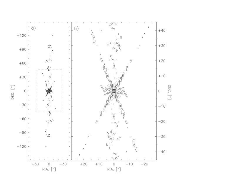
Figure 4: Representative synthesized beam belonging to pointing field 12 for a robust weighting of 0. a) Large field view with contours of 2.5, 5, 10, 20, 40 and 80% of the maximum. The dashed box outlines the area shown in b). b) Zoom into the central part of the synthesized beam with contours of 2, 4, 8, 16, 32, and 64% of the maximum. (The corresponding negative contours are shown in light gray.) The first peaks of the sidelobes are below 10% of the maximum, overall the shape of the synthesized beam is fairly well-behaved given the declination of the COSMOS field.

Figure 5: The COSMOS field as observed at 1.4 GHz. Bottom: The 2 deg² COSMOS field with the ACS coverage (from Scoville et al., 2006b) indicated by the gray box. The two green boxes outline the regions shown in the top panels. Top: Two regions enlarged demonstrate the quality of the data from the VLA-COSMOS large project. The left (right) panel represents the lower (upper) green box in the bottom panel. Each panel has a size of $2.8^{\prime}\times 2.8^{\prime}$ corresponding to about 0.1% of the total area.

Figure 6: Distribution of the noise. Pixel values extracted from a $16^{\prime}\times 11^{\prime}$ box close to the COSMOS field center show a Gaussian distribution in agreement with our assumption of Gaussian noise. The fitted Gaussian (dashed line) has a rms of $\rm 10.09\,\mu Jy/beam$ ($\sigma$) (i.e. a FWHM of $\rm 23.76\,\mu Jy/beam$). Noise distributions extracted from different boxes located through out the uniform part of the field look similar.

Figure 7: Comparison between the flux of the two calibrators 1024-008 and 0925+003 as a function of observing date. The dots show the peak flux density with indicated $3\sigma$ errors.

Figure 8: The peak flux density variations (dots) of the two observations per day for calibrator 0925+003 shown as a ratio of the measured peak flux densities. $3\sigma$ errors are indicated.

Figure 10: Distributions of $\Delta RA$ (thick dashed line) and $\Delta DEC$ (thin solid line) for different parts in the inner $0.87\Box^{\circ}$ area. The positions of the four panels in the diagram correspond exactly to the analyzed area. The mean and standard deviation of the offsets and the total number of sources are indicated in each panel. For clarity the pointing pattern of the VLA-COSMOS is shown in the background (dotted circles).

Figure 11: Fractional difference between the directly measured rms value in a $100\times 100$ pixel box and the corresponding value of the SExtractor noise map as a function of the radial distance for three different noise maps with mesh sizes of 25, 50 and 75 pixels, respectively. The x-positions have been shifted by 0.5^′ for clarity.

Figure 12: Sensitivity map of the area covered by the VLA Large Project derived using SExtractor with a mesh size of 50 pixel. The rms is fairly uniform except for areas around strong radio sources. Lighter shades indicate lower rms noise values. The contours correspond to rms levels of 10, 15, 20, 25, 30, and 40 $\mu$Jy/beam. The dashed box outlines the area which was searched for radio components.

Figure 13: Plot of the rms noise level vs. cumulative as well as fractional area covered. The full area covered is $\rm 2\,deg^{2}$ and is indicated in Fig. 12.

Figure 14: Map of the S/N of the VLA-COSMOS Large Project as constructed using the SExtractor sensitivity map (Fig. 12). Lighter shades indicate lower S/N values. The dashed box shows the area in which radio sources were identified (see also text).

Figure 17: Cumulative number distribution of the VLA-COSMOS sources as a function of peak (left) and integrated (right) flux density. The shaded area corresponds to sources that are resolved (see text).

Figure 18: Comparison of the derived integrated flux in the VLA-COSMOS large project $\rm I_{\rm VLA-COSMOS}$ and the NVSS and FIRST surveys $\rm I_{\rm external}$. The solid diagonal line represents a flux ratio of unity, while the dashed lines show the $\pm 20$% lines. The vertical lines denote the (5$\sigma$) detection limit of the NVSS and FIRST surveys (Condon et al., 1998; White et al., 1997). The counterparts to VLA-COSMOS sources lie within radii of $5^{\prime\prime}$ and $1^{\prime\prime}$ for the NVSS and FIRST survey, respectively. The large discrepancies in the derived integrated flux for several NVSS sources is likely due to the large difference in resolution (NVSS: $45^{\prime\prime}$ FWHM vs. VLA-COSMOS:$\sim\,1.5^{\prime\prime}$ FWHM), while the discrepancies in the integrated flux for the FIRST sources are mainly due to the fact that these are part of multi-component VLA-COSMOS sources.

References

- Afonso et al. (2005) Afonso, J., Georgakakis, A., Almeida, C., Hopkins, A. M., Cram, L. E., Mobasher, B., & Sullivan, M. 2005, ApJ, 624, 135
- Afonso et al. (2006) Afonso, J., Mobasher, B., Koekemoer, A., Norris, R. P., & Cram, L. 2006, AJ, 131, 1216
- Aguirre et al. (2006) Aguirre, J. E., et al. 2006, ApJS, this volume
- Appleton et al. (2004) Appleton, P. N., et al. 2004, ApJS, 154, 147
- Aretxaga et al. (2005) Aretxaga, I., Hughes, D. H., & Dunlop, J. S. 2005, MNRAS, 358, 1240
- Aussel et al. (2006) Aussel, H., et al. 2006, ApJS, this volume
- Becker et al. (1995) Becker, R. H., White, R. L., & Helfand, D. J. 1995, ApJ, 450, 559
- Benn et al. (1993) Benn, C. R., Rowan-Robinson, M., McMahon, R. G., Broadhurst, T. J., & Lawrence, A. 1993, MNRAS, 263, 98
- Bertin & Arnouts (1996) Bertin, E., & Arnouts, S. 1996, A&AS, 117, 393
- Bertoldi et al. (2006) Bertoldi, F., et al. 2006, ApJS, this volume
- Bondi et al. (2003) Bondi, M., et al. 2003, A&A, 403, 857
- Capak et al. (2006) Capak, P., et al. 2006, ApJS, this volume
- Carilli & Barthel (1996) Carilli, C. L., & Barthel, P. D. 1996, A&A Rev., 7, 1
- Carilli & Yun (2000) Carilli, C. L., & Yun, M. S. 2000, ApJ, 530, 618
- Ciliegi et al. (1999) Ciliegi, P., et al. 1999, MNRAS, 302, 222
- Condon (1992) Condon, J. J. 1992, ARA&A, 30, 575
- Condon (1997) Condon, J. J. 1997, PASP, 109, 166
- Condon et al. (1998) Condon, J. J., Cotton, W. D., Greisen, E. W., Yin, Q. F., Perley, R. A., Taylor, G. B.,Broderick, J. J. 1998, AJ, 115, 1693
- Condon et al. (2003) Condon, J. J., Cotton, W. D., Yin, Q. F., Shupe, D. L., Storrie-Lombardi, L. J., Helou, G., Soifer, B. T., & Werner, M. W. 2003, AJ, 125, 2411
- Ferguson et al. (2000) Ferguson, H. C., Dickinson, M., & Williams, R. 2000, ARA&A, 38, 667
- Fey et al. (2004) Fey, A. L., et al. 2004, AJ, 127, 3587
- Fomalont (1999) Fomalont, E. B. 1999, ASP Conf. Ser. 180: Synthesis Imaging in Radio Astronomy II, 180, 463
- Fomalont et al. (2006) Fomalont, E. B., Kellermann, K. I., Cowie, L. L., Capak, P., Barger, A. J., Partridge, R. B., Windhorst, R. A., Richards, E. A. 2006, ApJS, in press (astro-ph/0607058)
- Garrett (2002) Garrett, M. A. 2002, A&A, 384, L19
- Greisen (2003) Greisen, E. W. 2003, Information Handling in Astronomy - Historical Vistas, 109
- Gruppioni et al. (1999) Gruppioni, C., Mignoli, M., & Zamorani, G. 1999, MNRAS, 304, 199
- Haarsma et al. (2000) Haarsma, D. B., Partridge, R. B., Windhorst, R. A., & Richards, E. A. 2000, ApJ, 544, 641
- Hasinger et al. (2006) Hasinger, G., et al. 2006, ApJS, this volume
- Hopkins et al. (2003) Hopkins, A. M., Afonso, J., Chan, B., Cram, L. E., Georgakakis, A., & Mobasher, B. 2003, AJ, 125, 465
- Hopkins et al. (1998) Hopkins, A. M., Mobasher, B., Cram, L., & Rowan-Robinson, M. 1998, MNRAS, 296, 839
- Huynh et al. (2005) Huynh, M. T., Jackson, C. A., Norris, R. P., & Prandoni, I. 2005, AJ, 130, 1373
- Impey et al. (2006) Impey, C. D. et al. 2006, ApJS, this volume
- Ivezić et al. (2002) Ivezić, Ž., et al. 2002, AJ, 124, 2364
- Lilly et al. (2006) Lilly, S. et al. 2006, ApJS, this volume
- Norris et al. (2005) Norris, R. P., et al. 2005, AJ, 130, 1358
- Prandoni et al. (2001) Prandoni, I., Gregorini, L., Parma, P., de Ruiter, H. R., Vettolani, G., Wieringa, M. H., & Ekers, R. D. 2001, A&A, 365, 392
- Richards (2000) Richards, E. A. 2000, ApJ, 533, 611
- Roche et al. (2002) Roche, N. D., Lowenthal, J. D., & Koo, D. C. 2002, MNRAS, 330, 307
- de Ruiter et al. (1997) de Ruiter, H. R., et al. 1997, A&A, 319, 7
- Sadler et al. (2002) Sadler, E. M., et al. 2002, MNRAS, 329, 227
- Sanders et al. (2006) Sanders, D. B., et al. 2006, ApJS, this volume
- Schiminovich et al. (2006a) Schiminovich, D., et al. 2006a, ApJS, this volume
- Schinnerer et al. (2004) Schinnerer, E., et al. 2004, AJ, 128, 1974
- Scoville et al. (2006a) Scoville, N. Z., et al. 2006a, ApJS, this volume
- Scoville et al. (2006b) Scoville, N. Z., et al. 2006b, ApJS, this volume
- Smolčić et al. (2006) Smolčić, V., et al. 2006, ApJS, this volume
- Steidel et al. (1999) Steidel, C. C., Adelberger, K. L., Giavalisco, M., Dickinson, M., & Pettini, M. 1999, ApJ, 519, 1
- Taniguchi et al. (2006) Taniguchi, Y., et al. 2006, ApJS, this volume
- Trump et al. (2006) Trump, J. R., et al. 2006, ApJS, this volume
- White et al. (1997) White, R. L., Becker, R. H., Helfand, D. J., & Gregg, M. D. 1997, ApJ, 475, 479
- Windhorst et al. (1985) Windhorst, R. A., Miley, G. K., Owen, F. N., Kron, R. G., & Koo, D. C. 1985, ApJ, 289, 494