Radial stability of a family of anisotropic Hernquist models with and without a supermassive black hole

Abstract

We present a method to investigate the radial stability of a spherical anisotropic system that hosts a central supermassive black hole (SBH). Such systems have never been tested before for stability, although high anisotropies have been considered in the dynamical models that were used to estimate the masses of the central putative supermassive black holes. A family of analytical anisotropic spherical Hernquist models with and without a black hole were investigated by means of $N$-body simulations. A clear trend emerges that the supermassive black hole has a significant effect on the overall stability of the system, i.e. an SBH with a mass of a few percent of the total mass of the galaxy can prevent or reduce the bar instabilities in anisotropic systems. Its mass not only determines the strength of the instability reduction, but also the time in which this occurs. These effects are most significant for models with strong radial anisotropies. Furthermore, our analysis shows that unstable systems with similar SBH but with different anisotropy radii evolve differently: highly radial systems become oblate, while more isotropic models tend to form into prolate structures. In addition to this study, we also present a Monte-Carlo algorithm to generate particles in spherical anisotropic systems.

1 Introduction

Nowadays it is accepted that almost every galaxy hosts a central supermassive black hole (SBH) at its core. Since the kinematical discovery of the first SBH with the Hubble Space Telescope (HST), extensive studies have been carried out by many groups that investigate the demography of SBHs and the effect of the SBHs on their environment. The most popular discoveries are the correlations between the mass of the SBH ($M_{BH}$) and respectively the total blue magnitude $L_{B}$ of the hot stellar component in which it resides (Kormendy & Richstone, 1995), the central velocity dispersion of the hot stellar component (Ferrarese & Merritt, 2000; Gebhardt et al., 2000), the central light concentration $C(\alpha)$ or equivalent the Sérsic index $n$ (Graham et al., 2001) and the maximum rotational velocity of the galaxy (Ferrarese, 2002; Baes et al., 2003; Pizzella et al., 2005; Buyle et al., 2006). These relations have been calibrated with the known masses of the SBHs of the nearest galaxies, that mostly have been derived by means of either stellar or gas kinematics.

Sophisticated axisymmetric 3-integral dynamical models that allow a variation in mass-to-light ratio and anisotropy as a function of radius have been obtained by fits to the line-of-sight velocity distributions (LOSVDs) in the galaxies, which were derived primarily from high-resolution spectra taken with the HST

$$LOSVD\,(x,y,v_{z})=\frac{1}{\rho_{p}}\int\!\!\!\int\!\!\!\int F(\mn@boldsymbol{r},\mn@boldsymbol{v})\,dz\,dv_{x}\,dv_{y},$$ (1)

where $F(\mn@boldsymbol{r},\mn@boldsymbol{v})$ denotes the stellar distribution function (DF) and $\rho_{p}$ stands for the projected mass density at position $(x,y)$. The accuracy of the applied dynamical models to the observed stellar kinematics is still improving steadily and is reflected on the complexity of the DFs. Despite this positive progress on the dynamical front, very few anisotropic dynamical models of a galactic nucleus have been tested for dynamical stability (Ferrarese & Ford, 2005). One of the reasons for this is the complexity of the distribution functions, which are mostly numerically derived. Hence, to simulate these numerical DFs one normally approximates numerically the solution of the Jeans equations to derive the velocity dispersion profile and then uses Gaussians to provide local velocity distributions. It is now known from recent simulations of galactic systems that this method causes serious numerical artifacts (Kazantzidis et al., 2004).

So far the only theoretical analytical systems that contain a SBH are derived by Ciotti (1996) and Baes et al. (2004, 2005) where the attention is drawn primarily to the Hernquist model since this is the best-known approximation to the Sérsic profiles that are observed in bulges and elliptical galaxies, and by Stiavelli (1998) where the distribution function of a stellar system around an SBH is derived from statistical mechanic considerations. Ciotti (1996) initially starts with a 2-component system containing the luminous and dark matter and creates both isotropic and anisotropic (based on the Osipkov-Merritt strategy) systems. The dark matter halo (also represented by a Hernquist model) can be transformed into a central SBH by setting the core radius to zero.

In this article we present for the first time the results of a dynamical stability investigation of spherical systems containing an SBH, as a function of the mass of the SBH and the anisotropy radius of the system. We fill focus primarily on the so-called radial orbit instability of radially anisotropic, spherically symmetric stellar systems (Hénon, 1973; Cincotta et al., 1996). A beautiful mathematical and physical explanation for this instability can be found in Palmer (1994) and Merritt (1987) and references therein. As a bar grows, it saps angular momentum from the stars as they precess through the bar. Stars on low-angular momentum orbits are trapped into resonance and strengthen the bar, making it possible to also trap stars with higher angular momentum into resonance and so on. Eventually, the triaxial force field of the bar becomes dominant and the initially rosette-shaped orbits in a spherical potential are transformed into box orbits. Radial orbits and box orbits bring stars close to the center of the galaxy where they can be diverted from their orbits by the spherically symmetric force field of a central massive black hole. This in turn may weaken the bar over time, or even prevent it from forming in the first place, clearly proving the relevance of a study such as the one presented here.

In Section 2 we describe a Monte-Carlo algorithm that we developed to generate the initial conditions for the models, together with our $N$-body code and technique for investigating the stability. We present in Section 3 the results of a stability investigation of a family of anisotropic Hernquist models without an SBH, with different anisotropy behavior (Baes & Dejonghe, 2002). In Section 4 we describe the Osipkov-Merritt Hernquist models with a central SBH, introduced by Ciotti (1996). We investigate the stability of these systems in detail in Section 5, comparing them with the according models without an SBH. We perform this in a 2-parameter space as a function of the anisotropy radius $r_{a}$ and the mass of the central SBH $\mu$. In Section 6 we present our final results and conclusions.

2 Computational method

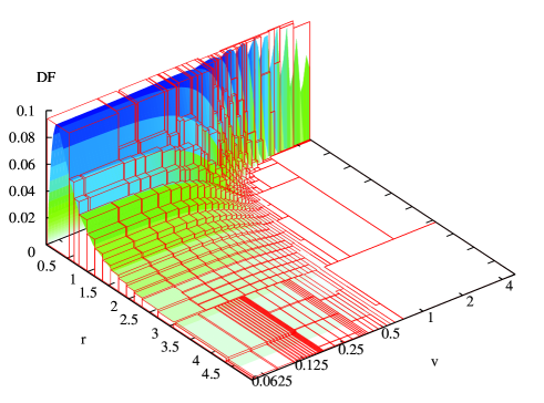
Figure 1: Visualization of an isotropic Hernquist system with $\mu=0.1$ and our approximation with cells. After 8 subdivisions 991 cells were constructed, with a total phase-space volume of $V_{8}=1.533$, while the real total stellar DF volume is 1. Thus, the ratio of rejected to accepted particles is $0.533$ and on average $\sim 35\%$ of all randomly chosen test particles in the cell volume will be rejected, resulting in a highly efficient Monte-Carlo simulation.

2.1 Definition of the Hernquist models

First of all we introduce some general characteristics of the models in our dynamical study. All systems are based on the spherical Hernquist potential-density pair (Hernquist, 1990), including a supermassive black hole in the centre. Given this mass profile, we shall investigate several distribution functions (DFs) consistent with the density outside the center, and which we will refer to as the stellar component. If we denote the total stellar mass by $M_{s}$, we can write the total mass as $M_{\mathrm{tot}}=M_{s}(1+\mu)$, where the fractional quantity $\mu$ determines the SBH mass $\mu M_{s}$. In our subsequent analysis we will work in dimensionless units $G=M_{s}=1$, so that the gravitating binding potential and the density are given by

$$\psi(r) = \frac{1}{1+r}+\frac{\mu}{r},$$ (2)

$$\rho(r) = \frac{1}{2\pi}\frac{1}{r(1+r)^{3}}\quad(r>0).$$ (3)

We will also express the time-steps in our $N$-body code (the time between two successive calculations) in dimensionless units of half-mass dynamical time, which is defined as the dynamical time (Binney & Tremaine, 1987) at the stellar half-mass radius:

$$T_{h}=\sqrt{\frac{3\pi}{16G\bar{\rho}}},$$ (4)

where

$$\bar{\rho}=\frac{3M(r_{1/2})}{4\pi r_{1/2}^{3}}.$$ (5)

For a Hernquist model with $\mu=0$ the half-mass dynamical time and the half-mass radius are

$$T_{h} = \frac{\sqrt{2}}{2}\pi\left(1+\sqrt{2}\right)^{3/2},$$ (6)

$$r_{1/2} = 1+\sqrt{2}.$$ (7)

We will also use these units for models with an SBH.

Figure 2: The figures show the relevant parameters ($\rho(r)$, $\sigma_{r}(r)$, $\sigma_{t}(r)$ and $\beta(r)$) of the outcome of a Monte Carlo sampling of a Hernquist system with $\mu=0.1$ and $r_{a}=1$. The continuous lines denote the theoretical model, the discrete data represent $10^{5}$ simulated particles, binned and with error-bars.

A conversion to observational units can be obtained through the close similarity between the Hernquist and De Vaucouleurs profiles (Hernquist, 1990), with $r_{1/2}\approx 1.33r_{e}$ where $r_{e}$ is the effective radius. Then a physical length, time and velocity are found by the scaling relations

$$\tilde{r} = \tilde{r}_{u}r,$$ (8)

$$\tilde{T}_{h} = \sqrt{\frac{\tilde{r}_{u}^{3}}{G\tilde{M}_{s}}}T_{h},$$ (9)

$$\tilde{v} = \sqrt{\frac{G\tilde{M}_{\mathrm{tot}}}{\tilde{r}_{u}}}v,$$ (10)

with $\tilde{M}_{s}$ the stellar mass, $\tilde{M}_{\mathrm{tot}}$ the total mass and $\tilde{r}_{u}=(1.33r_{e})/(1+\sqrt{2})$, expressed in physical units.

Every model was simulated by means of $10^{5}$ equal-mass particles that all follow the distribution function of the system and are contained within a sphere of radius $r_{b}=2000$ which encloses about 99.9% of the stellar mass of the system. We performed the simulations for 50 dynamical times, and used the values of the axis ratios $c/a$ and $b/a$ during this time as (in)stability indicators (see Section 2.4).

2.2 Constructing the data sets

Since we will investigate our models by means of $N$-body simulations, the first objective is to obtain representative discrete data sets from the considered distribution functions. Each of these functions describes a spherical mass distribution in a dynamical system governed by a gravitational binding potential $\psi(r)>0$, which implies that they can be expressed as functions $F(E,L)$ of the binding energy $E=\psi(r)-\frac{1}{2}v_{r}^{2}-\frac{1}{2}v_{t}^{2}$ and the modulus of the angular momentum $L=rv_{t}$, with $v_{r}$ and $v_{t}$ the radial and tangential velocity components, respectively. Isotropic DFs can be reduced to $F(E)$.

In order to extract discrete data samples from the distributions, we need to simulate random particles uniformly in the phase-space enclosed by the DFs. To this aim we used a Monte-Carlo simulator, developed by one of the authors (E.V.H.). The procedure works as follows: we write each DF as $F(r,v_{r},v_{t})$ and we consider a 4-dimensional grid space with $(r,v_{r},v_{t})$ as abscissae and the function values on the ordinate axis.

We start with a single cell in this space, extending from the origin to a boundary $(r_{b},v_{r,b},v_{t,b})$ (where $r_{b}$ is chosen to be sufficiently large, and $v_{r,b}=v_{t,b}=\sqrt{2\psi(0)}\,$), and with the ordinate set at the (known or estimated) DF maximum $f_{b}$. These boundaries (for infinite values a sufficiently large value is taken, see further) enclose a 7-dimensional phase-space volume

$$V_{1}=\bigg{(}\frac{4\pi}{3}r_{b}^{3}\bigg{)}\bigg{(}2v_{r,b}\bigg{)}\bigg{(}\pi v_{t,b}^{2}\bigg{)}f_{b}.$$ (11)

In the second step we attempt to split the cell into 8 sub-cells with different ordinates (i.e. the up to that point known function maxima in each cell). Therefore a co-ordinate $(r_{s},v_{r,s},v_{t,s})$ is sought to serve as the common corner point in the abscissae for these sub-cells: starting in the cell center, the total phase-space volume of the originating sub-cells is calculated, and through a number of iterations the cell is scanned for a better splitting point, i.e. which minimizes this volume. In this manner, the original cell is being split as efficiently as possible into 8 new cells, adding up to a new total volume

$$V_{2}\!\!\!\! = \!\!\!\!\sum_{i=1}^{8}V_{2;i},$$ (12)

$$= \!\!\!\!\sum_{i=1}^{8}\frac{8\pi^{2}}{3}(r_{b;i}^{3}\!-\!r_{a;i}^{3})(v_{r,b;i}\!-\!v_{r,a;i})(v_{t,b;i}^{2}\!-\!v_{t,a;i}^{2})f_{b;i},$$

which is a better approximation to the real DF volume. Here, for a cell $i$ we denoted $V_{2;i}$ its volume, $(r_{a;i},v_{r,a;i},v_{t,a;i})$ and $(r_{b;i},v_{r,b;i},v_{t,b;i})$ its lower and upper bounds in the abscissae, and $f_{b;i}$ its maximum DF value.

Next, each cell in our grid is examined according to the procedure above and split if it leads to a significant decrease in the total volume. Thus, after the examination of every cell, a new volume $V_{3}$ is obtained. This loop is repeated until after $M$ steps the phase-space volume $V_{M}$ has converged sufficiently close to the real volume. Typically, in our simulations, the cells cover a volume that is a factor 1.5 to 5 larger than the model’s actual phase-space volume; a further refinement is unnecessary, since constructing more cells would be more time-consuming than actually generating our desired number ($10^{5}$) of particles (see below). If the grid is successfully constructed, $F(r,v_{r},v_{t})$ is entirely enveloped by a set of 4-dimensional grid cells.

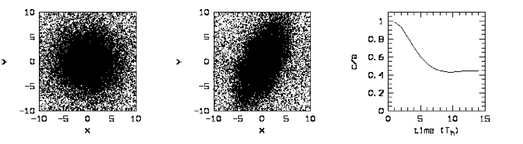
Figure 3: (a) The initial particle positions of a Hernquist model with an increasing anisotropy with $\beta=0.5$ and $\lambda=5$. 80% of the total mass is shown in the figure. (b) The density distribution after 10 half-mass dynamical times. A bar is clearly visible. (c) The axis ratio $c/a$ plotted as a function of time. As can be seen from both the density distributions and the axis ratio, an elliptical bar is created indicating that the system is unstable.

Now we can proceed to a classical rejection Monte-Carlo (MC) simulation (in the remainder, we refer to setting up the initial conditions of a DF as an “MC simulation”). To generate a data point $n$, first a value $V_{n}$ is randomly chosen between $0$ and $V_{M}$. We can associate this value with a unique cell $j$ and an ordinate $f_{n}$ for which

$$\sum_{i=1}^{j-1}V_{M;i}<V_{n}\leq\sum_{i=1}^{j}V_{M;i},$$ (13)

and

$$V_{n} \!\!\!=\!\!\! \sum_{i=1}^{j-1}V_{M;i}+$$ (14)

$$\frac{8\pi^{2}}{3}(r_{b;j}^{3}\!-\!r_{a;j}^{3})(v_{r,b;j}\!-\!v_{r,a;j})(v_{t,b;j}^{2}\!-\!v_{t,a;j}^{2})f_{n}.$$

Then, in cell $j$ the co-ordinates $r_{a;j}^{3}\leq r_{n}^{3}\leq r_{b;j}^{3}$ , $v_{r,a;j}\leq v_{r,n}\leq v_{r,b;j}$ and $v_{t,a;j}^{2}\leq v_{t,n}^{2}\leq v_{t,b;j}^{2}$ are randomly generated. Thus, a point $(r_{n},v_{r,n},v_{t,n},f_{n})$ is uniformly chosen in the 7-dimensional phase-space volume $V_{M}$. Now, if $f_{n}\leq F(r_{n},v_{r,n},v_{t,n})$, the co-ordinate $(r_{n},v_{r,n},v_{t,n})$ is accepted as a valid data point, otherwise it is rejected. Furthermore, if $f_{b;j}<F(r_{n},v_{r,n},v_{t,n})$, the cell volume is accordingly increased to the new maximum, so the grid keeps being improved.

In this manner we construct a data set of $N$ accepted co-ordinates inside the chosen radius $r_{b}$ which follow the distribution. The MC simulation is regarded successful if the cell volumes have changed negligibly (if the relative change of the total volume is smaller than $10^{-3}$) during the MC simulation. If not, a new MC simulation with the final grid (with volume $V_{M+N}$) is necessary. Also, if the ratio between rejected and accepted points is very large, causing the MC simulation to be slow, the grid might have to be refined further (as aforementioned, we stop refining the grid once the cells cover a volume that is a factor 1.5 to 5 larger than the model’s actual phase-space volume).

Finally, every co-ordinate $(r_{n},v_{r,n},v_{t,n})$ has to be converted into a phase-space point $(x_{n},y_{n},z_{n},v_{x,n},v_{y,n},v_{z,n})$. This is done by uniformly simulating the surface of a sphere with radius $r_{n}$ (creating $(x_{n},y_{n},z_{n})$), a circle with radius $v_{t,n}$ (creating $(v_{\theta,n},v_{\phi,n})$) and the sign of $v_{r,n}$. The velocities can then be transformed into the appropriate Cartesian co-ordinates. For isotropic functions $F(E)$ the grid abscissae simplify to the 2-dimensional $(r,v)$ space, and the entire procedure is analogous.

Our method has several advantages: the construction of a grid and the subsequent MC simulation of points is straightforward, fast, accurate and generally applicable. This contrasts with algorithms that require integrations and inversions of DFs, which can experience numerical problems with intricate functions. Also, no intermediate steps are required (e.g. simulating the density first before assigning velocities to each particle) and once a grid is made for a model, it can be re-used to generate an arbitrary number of particles. Moreover, since a peak can be adequately isolated by a cell, infinite ranges in the co-ordinate space or the DF values can be approximated by choosing appropriate large boundary values.

As an example we show in Fig. 1 the constructed cells for an isotropic Hernquist system with a central SBH of $\mu=0.1$ (see Section 4). A simulated data sample ($10^{5}$ accepted particles) for an anisotropic Hernquist system with a central SBH of $\mu=0.1$ and an anisotropy radius of $r_{a}=1$ is shown in Fig. 2. In all our MC simulations, we truncate the infinite boundary radius at $r_{b}=2000$. For the DFs with an infinite maximum, we set $f_{b}=10^{15}$, and for the SBH-models we set the maximum velocity at the arbitrarily large value $v_{b}=10^{15}$ (these values are in fact much larger than needed. In reality, no particle is ever assigned such a high DF value or initial velocity and never reaches such high velocities during the subsequent $N$-body simulations).

2.3 $N$-body code

We studied the stability of our models by using an $N$-body code that is based on the “self-consistent field” method (Hernquist & Ostriker, 1992). This method relies on the series expansion in a bi-orthogonal spherical basis set for both the density and gravitational potential

$$\rho(r,\theta,\phi) = \sum_{nlm}A_{nlm}\ \rho_{nlm}(r,\theta,\phi)$$ (15)

$$= \sum_{nlm}A_{nlm}\ \tilde{\rho}_{nl}(r)\ Y_{lm}(\theta,\phi),$$

$$\Phi(r,\theta,\phi) = \sum_{nlm}A_{nlm}\ \Phi_{nlm}(r,\theta,\phi)$$ (16)

$$= \sum_{nlm}A_{nlm}\ \tilde{\Phi}_{nl}(r)\ Y_{lm}(\theta,\phi),$$

where $Y_{lm}(\theta,\phi)$ are the spherical harmonics. Some freedom is considered for this expansion since ($\tilde{\rho}_{nl}(r)$,$\tilde{\Phi}_{nl}(r)$) can have different forms (e.g. Plummer model, Bessel functions, spherical harmonic functions), however here we will use a form similar to the Hernquist model due to its trivial connection with our anisotropic systems that we wish to examine:

$$\tilde{\rho}_{nl}(r) = \frac{K_{nl}}{\sqrt{\pi}}\frac{r^{l}}{r(1+r)^{2l+3}}C_{n}^{(2l+3/2)}(\xi),$$ (17)

$$\tilde{\Phi}_{nl}(r) = -2\sqrt{\pi}\frac{r^{l}}{(1+r)^{2l+1}}C_{n}^{(2l+3/2)}(\xi),$$ (18)

where $K_{nl}$ is a normalization constant, $\xi=(r-1)/(r+1)$ and $C_{n}^{(2l+3/2)}(\xi)$ are Gegenbauer polynomials (e.g. Szegö (1939), Sommerfeld (1964)). The coefficients $A_{nlm}$ can be calculated by means of all the particles that describe the DF of our system (see Hernquist & Ostriker (1992) for more details). The spherical accelerations for each particle are found by taking the gradient of the potential (eq. 16). Finally new positions and velocities are derived with the use of an integrator which is equivalent to the standard time-centred leapfrog (Allen & Tildesley, 1992; Hut et al., 1995),

$$x_{i+1} = x_{i}+\Delta tv_{i}+\frac{1}{2}\Delta t^{2}a_{i},$$ (19)

$$v_{i+1} = v_{i}+\frac{1}{2}\Delta t(a_{i}+a_{i+1}).$$ (20)

The indices $n$, ($l$, $m=-l...l$) are indirectly an indication for the accuracy of the simulation for respectively radial and tangential motion, since they determine the number of terms in the expansion (see Section 5.2 Hernquist & Ostriker (1992) for a statistical analysis). For the systems without the SBH we find that $n_{max}$=4 and $l_{max}$=2 assures a total energy conservation of better than $\sim 10^{-6}$ over 50 half-mass dynamical times $T_{h}$ and still allows a low CPU time per $N$-body time-step (the time between two successive calculations) of $\Delta t=T_{h}/416\approx 0.02$. For the systems with an SBH, we used $n_{max}=6,l_{max}=2$ when $\mu\leq 0.05$, and $n_{max}=8,l_{max}=4$ for larger values of $\mu$. The gravitational effect of the SBH is added analytically by an extra radial acceleration proportional to the mass of the SBH. To avoid numerical divergences when particles pass close to the SBH, we included a softening to this acceleration, i.e. $-\mu/(r^{2}+\epsilon^{2})$ with softening length $\epsilon=0.05$. At this radius the dynamical crossing time of a particle is $T_{h}=0.37$, which is still notably larger than our time-step of $0.02$. Adding this softening causes a discrepancy in the treatment of the SBH potential between the analytical models and the N-body code. As a consequence the initial conditions are not exactly in dynamical equilibrium so that the systems develop transient radial motions to adjust their density profile. However, this effect is marginal and does not influence the overall results. In all simulations with an SBH the energy is conserved better than 1% over 50 half-mass dynamical times.

In order to check the robustness of our results, we performed two kinds of tests. We (i) re-ran a number of simulations with different, smaller time-steps, and (ii) we performed simulations with higher $n_{max}$ and $l_{max}$ values. A detailed comparison of these extra runs with the original simulations shows that our results and conclusions do not change : the variation of the global instability indicators, such as axis ratios or $2K_{r}/K_{t}$, as a function of time are essentially the same.

2.4 Quantifying the instabilities

When a system is unstable, it tends to create a bar feature at its center (see Fig. 3) which roughly has an ellipsoidal shape. As noted by other authors (Merritt, 1987; Palmer & Papaloizou, 1987), the physical cause of instability is similar to that of the formation of a bar in a disc (Lynden-Bell, 1979), where a small perturbation changes the orbits with a lower angular momentum (initially precessing ellipses) into boxes which are aligned along the initiated bar. A particle in a box orbit is unable to precess all the way round and will fall each time back to the bar. This effect will cause the bar to increase in both size and strength. To measure the radial stability of the systems we fitted the shape of an ellipsoidal mass distribution by means of an iterative procedure (Dubinski & Carlberg, 1991; Katz, 1991; Meza & Zamorano, 1997; Meza, 2002) at every half-mass dynamical time. This detects any bar feature that is located within a given radius. The initial condition of this method is

$$\rho=\rho(a)\ \ \mathrm{with}\ \ a=\left(x^{2}+\frac{y^{2}}{q^{2}}+\frac{z^{2}}{s^{2}}\right)^{1/2},$$

and with $M_{ij}=\sum\frac{x_{i}x_{j}}{a^{2}}$, the principal components of the inertia tensor $M_{zz}\leq M_{yy}\leq M_{xx}$ and the axis ratios $q$ and $s$ equal to 1, assuming a spherical mass distribution within a certain sphere with a given radius for which we chose $r=5$. For all considered models this radius encloses approximately 70% of the total mass. To achieve these conditions a transition to the center of mass has to be made followed by swapping the coordinate axes into the correct order. In the next step the eigenvalues and eigenvectors of the inertia tensor $I_{ij}$ are calculated, transforming it into a diagonal matrix. At this point the new axis ratios can be calculated

$$q=\left(\frac{M_{yy}}{M_{xx}}\right)^{1/2}\!\!\!=\frac{b}{a}\ \ \mathrm{and}\ \ s=\left(\frac{M_{zz}}{M_{xx}}\right)^{1/2}\!\!\!=\frac{c}{a},$$ (21)

which in turn are used as the conditions for the next iteration step. The iteration was stopped as soon as both axis ratios converged to a value within a pre-established tolerance of $10^{-3}$. Thus at each half-mass dynamical time the values of these axis ratios serve as measures of the strength of the bar instability, if present.

3 Hernquist models without a black hole

In this section we investigate the stability of two different families of anisotropic Hernquist models without a central supermassive black hole. For the analytical construction of these models we refer to Baes & Dejonghe (2002), however we will recapitulate the characteristics of each family.

Figure 4: Axis ratios as a function of time of the anisotropic systems with a decreasing anisotropy.

3.1 Family I: Decreasing anisotropy

We find Hernquist models with a decreasing anisotropy by assuming an augmented density of the form

$$\tilde{\rho}(\psi,r)=\frac{1}{2\pi}\frac{\psi^{4-2\beta_{n}}}{(1-\psi)^{1-2\beta_{0}}}\frac{(1+r)^{2(\beta_{0}-\beta_{n})}}{r^{2\beta_{0}}},$$ (22)

with $\beta_{n}=\beta_{0}-\frac{n}{2}$ and $n$ a natural number. After some algebra we find the distribution function

$$F(E,L)\!\!\! = \!\!\!\frac{2^{\beta_{0}}}{(2\pi)^{5/2}}\Gamma(5-2\beta_{n})L^{-2\beta_{0}}E^{5/2-2\beta_{n}+\beta_{0}}$$ (23)

$$\times \!\!\!\sum_{k=0}^{n}\!{n\choose k}\!\frac{1}{\Gamma(\frac{2+k}{2}\!-\!\beta_{0})\Gamma(\frac{7-k}{2}\!-\!2\beta_{n}\!+\!\beta_{0})}\!\!\left(\!\frac{L}{\sqrt{2E}}\!\right)^{k}$$

$$\times \!\!\!{}_{2}F_{1}\left(5\!-\!2\beta_{n},1\!-\!2\beta_{0};\frac{7-k}{2}\!-\!2\beta_{n}\!+\!\beta_{0};E\right),$$

with ${}_{2}F_{1}$ a hypergeometric function (see Appendix A), and the anisotropy

$$\beta(r)=1-\frac{\sigma^{2}_{t}(r)}{\sigma_{r}^{2}(r)}=\frac{\beta_{0}+\beta_{n}r}{1+r},$$ (24)

which decreases as a function of radius. Since for $\beta_{0}\leq 0$ we only find tangentially dominated systems which are free of radial instabilities, we limit ourselves to the investigation of the case $\beta_{0}=0.5$. For this value, $n=0$ corresponds to a system with constant anisotropy. We plotted the axis ratios $c/a$ for a number of different models with different $n$ in Fig. 4. Here and in the remainder of the paper, we define those models that keep the axis ratio $c/a\gtrsim 0.95$ over 50 dynamical times as being stable. The only model that does not satisfy this criterion is that with $n=1$, which is everywhere radially anisotropic. For $n\geq 2$, the models become tangentially anisotropic at larger radii and as a consequence are much more stable. This is evident from Fig. 4. It is clear that the minimum of $c/a$ is reached rapidly, whereafter the systems are in an equilibrium state, but are slightly non-spherical.

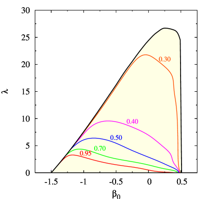
Figure 5: The stability of the Hernquist models without a black hole and with increasing anisotropy (see Section 3.2), expressed as the minima of the axis ratios $c/a$ during the simulations. The shaded area indicates the region of physical systems, i.e. with a non-negative distribution function.

Figure 6: The distribution functions defined by Ciotti (1996), with different anisotropy radii $r_{a}$ and SBH mass $\mu$. The value $r_{a}=\infty$ corresponds with the isotropic case; for $\mu=0$ the DFs reduce to eq. (28).

3.2 Family II: Increasing anisotropy

These models are a generalization of the Osipkov-Merritt models (Cuddeford, 1991) with an augmented density and DF of the general form

$$\tilde{\rho}(\psi,r)\!\!\! = \!\!\!r^{-2\beta_{0}}f(\psi)\left(1+\lambda r^{2}\right)^{-1+\beta_{0}}\ \ \textrm{with}\ \ \lambda=\frac{1}{r_{a}^{2}},$$ (25)

$$F(E,L)\!\!\! = \!\!\!F_{0}(Q)L^{-2\beta_{0}}\ \ \textrm{with}\ \ 0\leq Q=E-\frac{L^{2}}{2r_{a}^{2}}\leq 1,$$ (26)

and $E$ denotes the energy, $L$ the angular momentum and $r_{a}$ the anisotropy radius. The explicit form of $f(\psi)$ for the Hernquist potential-density pair can be found in Baes & Dejonghe (2002). As mentioned by them, the DFs can be written analytically for the half-integer values $\beta_{0}=0.5,0,-0.5,-1$, so we will limit ourselves to these cases. For every value of $\beta_{0}$, we also computed numerically the maximum anisotropy value $\lambda_{\mathrm{max}}(\beta_{0})$, outside which the DFs become negative for some values of $Q$ and $L$. The area of physical systems is indicated in Fig. 5. Our models have the following functional form:

• $\beta_{0}=0.5$:

  $$F(E,L)=\frac{Q}{4\pi^{3}L}\frac{3Q^{2}+\lambda(3Q^{2}-5Q+2)}{\sqrt{Q^{2}+\lambda(1-Q)^{2}}}.$$ (27)

• $\beta_{0}=0$:

  $$F(E,L)\!\!\! = \!\!\!\frac{1}{8\sqrt{2}\pi^{3}}\left[\frac{3\arcsin{\sqrt{Q}}}{(1-Q)^{5/2}}\right.$$ (28)

  $$\!\!\!+\left.\sqrt{Q}(1-2Q)\left(\frac{8Q^{2}-8Q-3}{(1-Q)^{2}}+8\lambda\right)\;\right].$$

• $\beta_{0}=-0.5$:

  $$F(E,L)=\frac{Lf(Q)}{4\pi^{3}(1-Q)^{4}\sqrt{Q^{2}+\lambda(1-Q)^{2}}},$$ (29)

  with

  $$f(Q) = 6(1+\lambda)^{2}Q^{6}-2(16\lambda^{2}+26\lambda+10)Q^{5}$$ (30)

  $$+(70\lambda^{2}+87\lambda+20)Q^{4}-2\lambda(40\lambda+33)Q^{3}$$

  $$+\lambda(50\lambda+19)Q^{2}-16\lambda^{2}Q+2\lambda^{2}.$$

• $\beta_{0}=-1$:

  $$F(E,L) = \frac{L^{2}}{256\sqrt{2}\pi^{3}(1-Q)^{5}}\times$$ (32)

  $$\left[\frac{f_{1}(Q)}{\sqrt{1-Q}}\arctan\left(\frac{\sqrt{Q}}{\sqrt{1-Q}}\right)+\frac{f_{2}(Q)}{\sqrt{Q}}\right],$$

  with

  $$f_{1}(Q)=15\left[(16\lambda+120)Q^{2}-(72+32\lambda)Q+15+16\lambda\right],$$ (33)

  $$f_{2}(Q) = 384(1+\lambda)^{2}Q^{6}$$ (34)

  $$-(1984\lambda^{2}+3712\lambda+1728)Q^{5}$$

  $$+(4160\lambda^{2}+7008\lambda+2784)Q^{4}$$

  $$-(4480\lambda^{2}+6192\lambda+1200)Q^{3}$$

  $$+(2560\lambda^{2}+2368\lambda+930)Q^{2}$$

  $$-(704\lambda^{2}+240\lambda+225)Q+64\lambda^{2}.$$

For all models the anisotropy is given by the simple formula

$$\beta(r)=\frac{r^{2}+\beta_{0}r_{a}^{2}}{r^{2}+r_{a}^{2}},$$ (35)

showing an increase in anisotropy as a function of radius. The results of the $N$-body investigation for all $\beta_{0}$ and $\lambda$ are summarized in figure 5, where we plotted the minimal axis ratios $c/a$ for the DFs in this parameter space. To derive this plot, we simulated systems with $\beta_{0}=0.5,0,-0.5,-1$ and $\lambda=1,2,4,6,10,16,24$ where physically possible. The case where $\beta_{0}=0$ corresponds to the traditional anisotropic Osipkov-Merritt Hernquist model that has been previously investigated in a similar way by Meza & Zamorano (1997). These authors state the system with $r_{a}\approx 1.1$ (or $\lambda\approx 0.82$) as stable. To compare our study with theirs, we simulated this model in addition to the other systems. For this model we find an axis ratio $c/a\approx 0.95$ after 50 dynamical times, and $2K_{r}/K_{t}\approx 2.2$ during the entire run. These values are in agreement with their results, therefore we will define $c/a=0.95$ as our stability criterion.

As is to be expected, the anisotropy radius $\lambda$ strongly affects the formation of radial-orbit instabilities, so that only models with a low value of $\lambda$ remain stable. Furthermore we note that all models remain in their new equilibrium state after $t\approx 10T_{h}$, as in case of the DFs of Family I. As an example, the $c/a$ ratio evolution for one of the systems is given in Fig. 3.

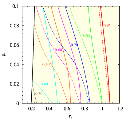
Figure 7: Contour plot of the axis ratio $c/a$ for the Osipkov-Merritt models as a function of anisotropy radius and mass of the SBH. The shaded area indicates the region of physical systems, i.e. with a non-negative distribution function. The solid lines indicate the minimal values during the simulation, the dashed lines show the axis ratios at the end of the simulation (at $t=50T_{h}$).

4 Hernquist models with a supermassive black hole

The now established presence of diverse components in a great variety of galaxies calls for more advanced dynamical models. In this respect a dark matter halo and a central supermassive black hole are important and can change the galaxy’s properties dramatically. However, up to now there are few known analytical systems that include e.g. a supermassive black hole. The only models known so far are presented in Ciotti (1996), Baes & Dejonghe (2004) and Baes et al. (2005) which are all based on the $\gamma$-models with special attention to the Hernquist model and in Stiavelli (1998) where the distribution function of a stellar system around an SBH is derived from statistical mechanic considerations.

In this section we investigate the radial stability of both isotropic and anisotropic Hernquist models containing a supermassive black hole, as these represent the closest analytical approach to the observations. For the following sections we will use the representation of Ciotti (1996); again, we are not going into great detail in the derivation of the analytical distribution function.

In essence the DFs are obtained from an analytical Osipkov-Merritt inversion of the systems governed by eq. (2) and (3). As a consequence, these models can be viewed as a extension of eq. (28). Subsequently, we will refer to these combined systems as Osipkov-Merritt models. The DFs can be written as

$$F(Q)=F_{i}(Q)+\frac{F_{a}(Q)}{r_{a}^{2}},$$ (36)

where $Q$ has the same definition as in eq. (26). A more natural parameter $q$ is defined through

$$Q=q\left(1+\frac{\mu}{1-q}\right),\quad 0\leq q\leq 1.$$ (37)

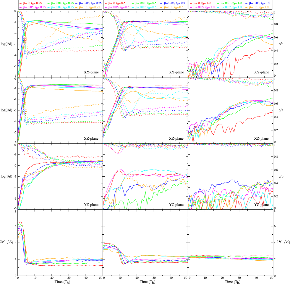
Figure 8: The evolution of systems with an anisotropy radius of respectively $r_{a}=0.25,0.50,1.0$, but with different mass of the SBH ($\mu=0,0.01,0.03,0.05,0.07,0.1$). For each column we plot the evolution of the axes ratios (dashed lines) and Fourier coefficients (full lines) in the upper three rows. The bottom row contains the evolution of the $2K_{\perp}/K_{\parallel}$ ratio as a function of dynamical time ($T_{h}$).

4.1 Family I: Isotropic

We find an isotropic system by letting $r_{a}$ diverge to $\infty$. Then eq. (36) simplifies to

$$F(E)=F_{i}(E)=\frac{1}{2\sqrt{8}\pi^{3}}\left(\frac{dE}{dl}\right)^{-1}\frac{d}{dl}\left[\tilde{F}_{i}^{\pm}(l)\right],$$ (38)

with the argument $l$ defined as $l^{2}=1-q$. For $\tilde{F}_{i}^{\pm}(l)$ we refer to Ciotti (1996) as this involves combinations of elliptic and Jacobian functions. These models only differ from those of Baes et al. (2005) in the definition of the parameter $\mu$.

Although the systems are isotropic, their DFs have a local maximum when $\mu>0$ (as shown in Fig. 6). Hence, the sufficient criteria of Antonov (1962) and Dorémus and Feix (1973) for isotropic systems cannot be applied. However, in our subsequent analysis of the systems with and without an SBH in Section 5, it will be shown that all models with $r_{a}>1$ are stable. In other words, it becomes evident that the addition of a central SBH, although it changes the dynamics dramatically, does not influence the density distribution of an isotropic system.

4.2 Family II: Anisotropic

In a similar way as the isotropic case the distribution function can be written as

$$F(Q) = F_{i}(Q)+\frac{F_{a}(Q)}{r_{a}^{2}},$$ (39)

$$= \frac{1}{2\sqrt{8}\pi^{3}}\left(\frac{dQ}{dl}\right)^{-1}\frac{d}{dl}\left[\tilde{F}_{i}^{\pm}(l)+\frac{\tilde{F}_{a}^{\pm}(l)}{r_{a}^{2}}\right],$$ (40)

where again $\tilde{F}_{a}^{\pm}(l)$ is defined in Ciotti (1996). In Fig. 6 we display systems with several values of $\mu$ and $r_{a}$. Notice that for small values of $r_{a}$ the DFs have a local minimum. As a consequence, for every $\mu$ there exists a smallest possible $r_{a}$, where this minimum becomes zero; smaller values of this boundary $r_{a}$ result in negative DFs, thus creating unphysical systems. For $\mu=0$, the minimal anisotropy radius is $r_{a}\approx 0.202$; for $\mu=0.1$ the boundary becomes $r_{a}\approx 0.240$. From the viewpoint of a stability analysis these systems are the most interesting. In the following section we will discuss their evolution in detail, comparing them with the models without an SBH (eq. (28)).

5 Stability analysis of the Osipkov-Merritt models

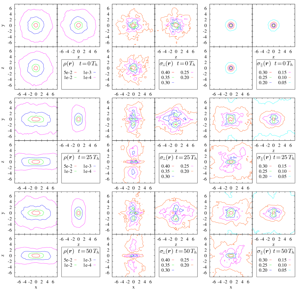
Figure 9: The spatial density $\rho$ and the velocity dispersions $\sigma_{\!\perp}$ and $\sigma_{\parallel}$, in the three principal planes, of an Osipkov-Merritt Hernquist system without an SBH, and with $r_{a}=0.25$. Dynamical times $t=0$, $t=25T_{h}$ and $t=50T_{h}$ are displayed.

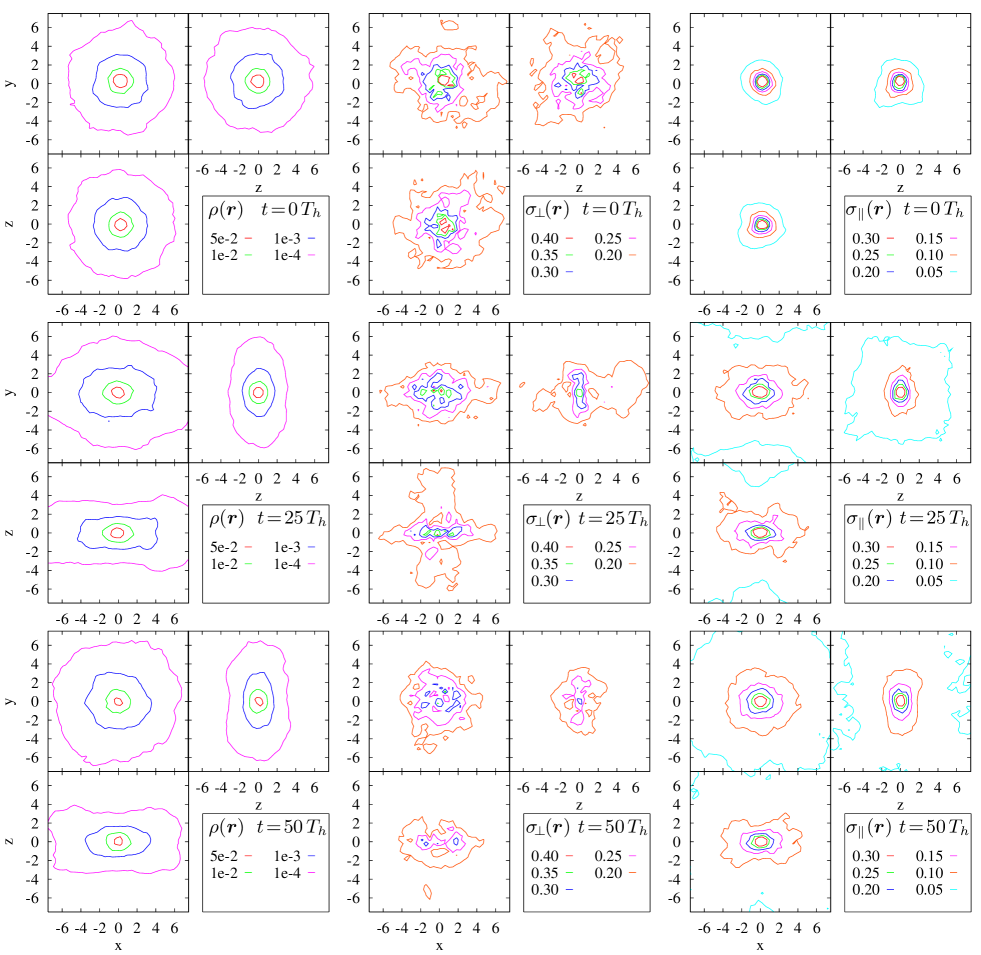
Figure 10: The spatial density $\rho$ and the velocity dispersions $\sigma_{\!\perp}$ and $\sigma_{\parallel}$, in the three principal planes, of an Osipkov-Merritt Hernquist system with an SBH of $\mu=0.05$, and with $r_{a}=0.25$. Dynamical times $t=0$, $t=25T_{h}$ and $t=50T_{h}$ are displayed.

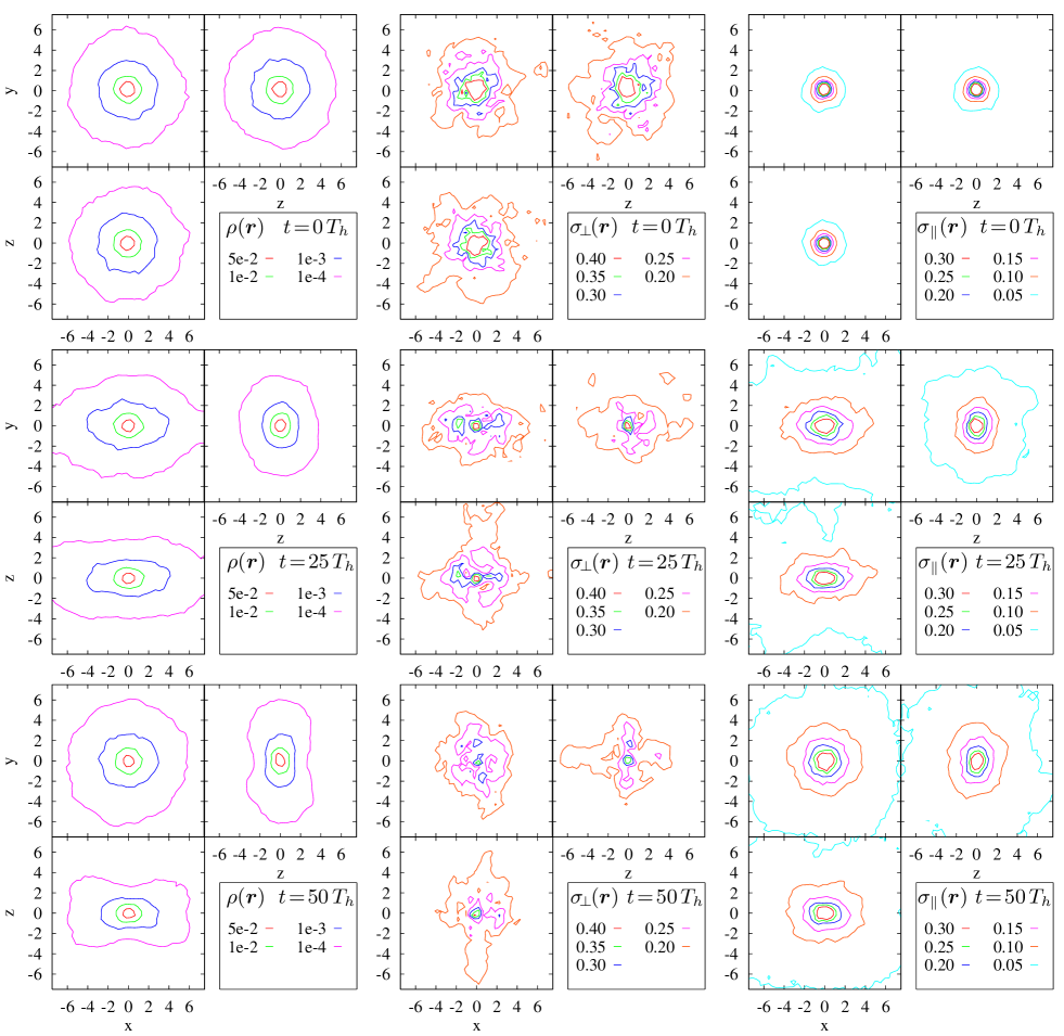
Figure 11: The spatial density $\rho$ and the velocity dispersions $\sigma_{\!\perp}$ and $\sigma_{\parallel}$, in the three principal planes, of an Osipkov-Merritt Hernquist system with an SBH of $\mu=0.1$, and with $r_{a}=0.25$. Dynamical times $t=0$, $t=25T_{h}$ and $t=50T_{h}$ are displayed.

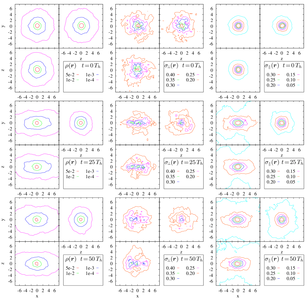
Figure 12: The spatial density $\rho$ and the velocity dispersions $\sigma_{\!\perp}$ and $\sigma_{\parallel}$, in the three principal planes, of an Osipkov-Merritt Hernquist system with an SBH of $\mu=0.05$, and with $r_{a}=0.50$. Dynamical times $t=0$, $t=25T_{h}$ and $t=50T_{h}$ are displayed.

To investigate any trend about the radial stability of these systems, we investigate the 2-parameter space ($r_{a}$,$\mu$). In total, we performed 25 simulations, with $r_{a}=0.25,0.50,0.70,0.85,1.00$ and $\mu=0.01,0.03,0.05,0.07,0.10$. This way we derived a grid of values of the $c/a$ axis ratios, shown in Fig. 7. As stated before, the ($\mu=0$)-axis corresponds to the systems in eq. (28). The solid lines indicate the minimal values reached during the simulation (i.e. when the instability is strongest). The rate at which these minima are reached strongly depends on $r_{a}$, ranging from a few half-mass dynamical times for highly radial models to $t\approx 50T_{h}$ for systems with $r_{a}=1.00$. After the point of time upon which a system obtains its minimal $c/a$ the influence of the SBH causes a diminution of the bar instability, resulting in the $c/a$ axis ratios at $t=50T_{h}$ shown by the dashed lines. Thus, in each system the particles are affected by two counteracting forces: the (relatively fast) bar formation and the (more gradually) scattering near the center due to the spherically symmetric gravitational potential of the black hole. The contour line $c/a=0.95$ is highlighted as our stability criterion.

A full dynamical analysis would require a detailed study of the orbital distribution of the stellar mass. However, we can gain important insights into the dynamics of the models by visualizing the evolution of various quantities, in Figs. 8-12.

First, in order to retain a notion of ’radial’ and ’tangential’ motion in an evolved system (resembling a triaxial model) at a certain time $t$ , we use the method described in Section 2.4 to approximate the mass distribution inside the radius $r_{i}$ of each particle by an ellipsoid. Then, the velocity of a particle can be written into two components perpendicular resp. parallel to its surface $v_{i}=v_{i,\perp}+v_{i,\parallel}$. Subsequently, the perpendicular and parallel velocity dispersion of the $m$ nearest neighbors around a position $\mn@boldsymbol{r}$ are

$$\sigma^{2}_{\perp}(\mn@boldsymbol{r}) = \frac{1}{m-1}\sum_{i=1}^{m}\big{(}v_{i,\perp}-\bar{v}_{\perp}\big{)}^{2},$$ (41)

$$\sigma^{2}_{\parallel}(\mn@boldsymbol{r}) = \frac{1}{2(m-1)}\sum_{i=1}^{m}\big{(}v_{i,\parallel}-\bar{v}_{\parallel}\big{)}^{2}.$$ (42)

In a similar manner we define

$$K_{\perp} = \frac{1}{N}\sum_{i=1}^{N}v_{i,\perp}^{2},$$ (43)

$$K_{\parallel} = \frac{1}{N}\sum_{i=1}^{N}v_{i,\parallel}^{2},$$ (44)

so that $2K_{\perp}/K_{\parallel}$ can serve as a non-spherical extension of $2K_{r}/K_{t}$.

In Fig. 8 we compared our $c/a$ criterion to other known methods to quantify the stability of the system. For all our systems with $r_{a}$ = 0.25, 0.50 and 1.0, we plot the evolution of the three axis ratios against the Fourier coefficient (Sellwood & Merritt, 1994) in the three principal planes (XY, XZ and YZ), and the evolution of $2K_{\perp}/K_{\parallel}$(t). The Fourier coefficient in a plane is defined as

$$A=\frac{1}{N}\sum_{j}e^{2i\theta_{j}},$$ (45)

with $\theta_{j}$ the azimuth of particle $j$ in this plane. Together with the $2K_{\perp}/K_{\parallel}$ ratio it is widely used as a measurement of the instability of a system. From this figure it is clear that all 3 methods indicate a similar result. For the models $r_{a}=1.0$ (right column) the axis ratios and the $2K_{\perp}/K_{\parallel}(t)$ ratio remain nearly constant during the entire run, while the Fourier coefficient either remains constant or increases upto a very low value and then slowly declines, indicating no further evolution in the stability has to be expected. Only the systems with $\mu=0$ and $\mu=0.01$ have moderately increasing Fourier coefficients, indicating a marginal, slowly evolving instability; models with higher $\mu$ can be considered stable.

Lower values of the anisotropy radius $r_{a}$ leads to unstable systems; in columns 1 and 2 we display all systems with respectively $r_{a}=0.25$ and $r_{a}=0.5$. Clearly, the rate at which the bar is created depends strongly on $r_{a}$. During a simulation of an unstable system the $2K_{\perp}/K_{\parallel}(t)$ ratio rapidly reaches a maximum and then declines to a value of $\approx 2.0$ after which it remains constant for the remainder of the run. This maximum is an artifact of the softening applied in the N-body simulation and is caused by the fact that the initial conditions are not exactly in dynamical equilibrium (see Sect. 2.3). Lowering the time-step and softening length caused a diminution of the maxima. The time at which the $2K_{\perp}/K_{\parallel}$ ratio reaches this constant value corresponds with the time the axis ratios reach their lowest value and the Fourier coefficients reach their highest value. The influence of the mass of an SBH is more clearly visible in the axis ratios and Fourier coefficients. A remarkable result is the difference between the systems $r_{a}=0.25$ and $r_{a}=0.5$ in the evolution of the axis ratios: the former models first become triaxial, after which $b/a$ increases and $c/b$ decreases. The latter models are prolate axisymmetric during the entire run.

In summary, an SBH mass of a few percent can prevent or reduce the bar instabilities in anisotropic systems. This result agrees well with similar studies in disk galaxies (Norman et al., 1996; Shen & Sellwood, 2004; Athanassoula et al., 2005; Hozumi & Hernquist, 2005). The effect is strongest for models with strong radial anisotropies, where the decrease of the bar strength is proportional to the SBH mass. In other words, while more radially anisotropic systems develop stronger bars than more isotropic models, the bars of the former are more easily affected by a supermassive black hole (see Fig. 8). This is to be expected, since radial systems host more eccentric orbits, therefore more particles from the outer regions pass near the center where their orbits can be altered by the Kepler force of the SBH.

An alternative approach to present the evolution of the models is given in Figs. 9-12, where we show the evolution of 4 systems by means of the density $\rho(\mn@boldsymbol{r})$ and velocity dispersions $\sigma_{\!\perp}(\mn@boldsymbol{r})$ and $\sigma_{\parallel}\,(\mn@boldsymbol{r})$, in at dynamical times $t=0,\ t=25T_{h}$ and $t=50T_{h}$. In each principal plane the moments are calculated on a grid of 2500 points, with 50 nearest neighbors around every grid position.

Fig. 9 displays an Osipkov-Merritt system without an SBH and anisotropy radius $r_{a}=0.25$. As was shown in Fig. 8 this model has a strong bar formation, resulting into a new equilibrium state after $t=5T_{h}$ which it retains during the rest of the run (as can be seen at $t=25T_{h}$ and $t=50T_{h}$). This bar alters the density distribution into a roughly triaxial symmetry, even peanut-shaped in the $XZ$-plane where the radial instability is the most prominent. The tangential dispersion $\sigma_{\parallel}$ increases significantly. This occurs especially at the edges, where in contrast the radial dispersion vanishes. This can be explained by the mechanism of the bar formation: particles that pass through the bar are pulled towards it, and eventually align their orbit with the bar. Only the orbits along the principal axes remain largely unaffected by the bar due to the symmetric forces on these particles, hence their motion remains radial.

In Fig. 10 a model with $r_{a}=0.25$ and $\mu=0.05$ is shown. Again a bar is formed, but less pronounced than in the absence of an SBH. Clearly, during the run the bar is reduced by the SBH, causing a gradual increase in the $c/a$ axis ratio ($XZ$-plane). More striking however is the evolution in the $XY$-plane, where the ellipticity has disappeared. Thus, the model has become an oblate axisymmetric system. This is also reflected in the dispersions: $\sigma_{\parallel}$ again follows the bar structure, but the cross-form $\sigma_{\!\perp}$ vanishes as particles pass near the SBH. Since most particles reside in the $XY$-plane, on eccentric orbits (since $r_{a}$ is small), the scattering in this plane is strongest. After $t=50T_{h}$, we expect a further small increase in the $c/a$ axis ratio, but as the velocity dispersion becomes more isotropic fewer particles from the outer regions will pass near the center (i.e. be affected by the SBH), hence the model will not change much further.

This can also be seen by comparing the system with $\mu=0.05$ to a model with $\mu=0.1$ (Fig. 11). This model has essentially the same properties as the former. The larger SBH mass has above all influence on its efficiency, resulting in a faster bar reduction.

Finally, we consider the effect of the anisotropy radius by analyzing a system with $\mu=0.05$ and $r_{a}=0.5$ (Fig. 12). Compared to Fig. 10, the initial bar is less strong, as expected. However, its structure and evolution is different from the system with $r_{a}=0.25$. First, $\sigma_{\!\perp}$ remains spherically distributed during the run, thus less scattering occurs. This implies less reduction of the bar instability. Moreover, the density does not become symmetric around the $Z$-axis. In contrast, the $X$-axis is now the symmetry axis during the entire run, resulting in a prolate axisymmetric system. It thus seems that models with an SBH become oblate or prolate, depending on their velocity anisotropy. It would indeed be very interesting to compare the orbital structure of both these systems in full detail.

As a final remark we note that inside a radius $r_{K}=\sqrt{\mu}/(1-\sqrt{\mu})$ the force of the SBH is stronger than the stellar component, so that all models remain spherical inside this radius. In conclusion, systems with an SBH become axisymmetric systems with a spherically symmetric core.

6 Conclusions and summary

Most mass estimates of SBHs result from dynamical models of either stellar or gas kinematics. The inclusion of strong radial anisotropy is considered in these models (Binney & Mamon, 1982), yet they have never been tested for radial stability. Our goal was to test the stability of systems with a central SBH and to look for any trend as a function of the mass of the SBH. We used the same method that was previously introduced by Meza & Zamorano (1997) and extended it to systems with a central SBH. We first tested the procedure on Hernquist systems (Baes & Dejonghe, 2002) without an SBH and with different anisotropic behavior. Our method appeared to be efficient in discriminating the stable from the unstable systems.

Instead of focusing on complicated numerically derived dynamical models, we opted for analytical distribution functions that take the effect of a central SBH into account, in order to be able to look for any trend. Since the isotropic Hernquist models with an SBH do not have distribution functions that are monotonically increasing functions of the binding energy (Ciotti, 1996; Baes & Dejonghe, 2004) and hence the sufficient criteria of Antonov (1962) and Dorémus and Feix (1973) for isotropic systems cannot be applied, we first investigated the radial stability of these systems. No effect was found by letting the mass of the SBH vary, giving only stable systems. However, in the case of the anisotropic systems with an SBH we did find a dependence of the stability of the system on the mass of the SBH. The more massive the SBH, the more stable a system becomes, but especially the more the instability is reduced. A trend which is most obvious in very anisotropic systems (thus with very small anisotropy radius $r_{a}$). An SBH with a mass of a few percent of the entire galaxy mass, is able to weaken the strength of the bar, which is in correspondence with similar studies in disk galaxies (Norman et al., 1996; Shen & Sellwood, 2004; Athanassoula et al., 2005; Hozumi & Hernquist, 2005). Judging from Fig. 7, the stability boundary of $c/a\gtrsim 0.95$ over 50 dynamical times, shifts from $r_{a}\approx 1.1$ for $\mu=0$ to $r_{a}\approx 1.0$ for $\mu=0.1$. This corresponds to $2K_{r}/K_{t}=2.2$ for $\mu=0$ and to $2K_{r}/K_{t}=2.0$ for $\mu=0.1$. These values are in very good agreement with previous authors.

Remarkably, systems with an SBH but with different anisotropy radii $r_{a}$ evolve differently: highly radial systems first become triaxial whereafter the SBH makes them more oblate if $\mu$ is large, while less radial models tend to form first into axisymmetric prolate structures, that then become less elongated due to the influence of the SBH.

It is also interesting to note that the central density distribution of systems with an SBH remains spherically symmetric during the entire simulation out to a radius of half the effective radius. This is not the case for systems without an SBH, which become axisymmetric or triaxial, depending on $r_{a}$. Interestingly, this includes the region that is considered for the $M_{BH}-\sigma$ relation, which predicts such an evolutionary link between the central SBH and the spheroid where it resides. Similarly, the central anisotropy parameter decreases as a function of time at a rate proportional to the mass of the SBH, due to more tangential orbits at the center.

Apart from a central SBH, one can also investigate the effect of central density cusps (Sellwood & Evans, 2001; Holley-Bockelmann et al., 2001) or isotropic cores (Trenti & Bertin, 2006) on the radial stability. Previous research shows that both central density cusps and isotropic cores act as dynamical stabilizers, hence the same effect as the addition of an SBH. In the future we plan to look at the combination of both investigations, namely the combination of an SBH and central density cusp.

Ultimately, one can of course verify the radial stability of the state-of-the-art models that are being used to estimate the mass of the SBHs with e.g.our methodology, however this investigation was not the goal of this paper.

Appendix A Hypergeometric function

A relevant definition of Generalized hypergeometric functions ${}_{p}F_{q}(a_{1},\ldots a_{p};b_{1},\ldots,b_{q};x)$ can be found in Gradshteyn & Ryzhik Sec. 9.14, page 1071 in the 5th edition. For specific arguments hypergeometric functions can be reduced to more simpler analytical functions, this can be done with mathematical software packages as e.g. Maple or Mathematica. For general coefficients however, the evaluation needs to be done by means of hypergeometric series:

$${}_{p}F_{q}(a_{1},\ldots,a_{p};b_{1},\ldots,b_{q};x) = 1+\sum_{j=0}^{+\infty}$$

$$\prod_{k=0}^{j}\frac{x\prod_{i=1}^{p}(a_{i}+k)}{(1+k)\prod_{i=1}^{q}(b_{i}+k)}.$$

This routine is very suitable to numerically evaluate any generalized hypergeometric function within a certain degree of accuracy.

References

- Allen & Tildesley (1992) Allen, M. P., & Tildesley, D. J. 1992, Computer Simulation of Liquids (Oxford: Oxford Univ. Press)
- Antonov (1962) Antonov, V. A. 1962, Vestnik Leningrad University, 19, 96 (trans. in Princeton Plasma Physics Lab. Rept. PPl-Trans-1 and Goodman, J., & Hut, P. ed. 1985. Dynamics of Star Clusters, IAU Symposium No. 113. Dordrecht: Reidel)
- Athanassoula et al. (2005) Athanassoula, E., Lambert, J. C., & Dehnen, W. 2005, MNRAS, 363, 496
- Barnes et al. (1986) Barnes, J., Hut, P., & Goodman, J. 1986, ApJ, 300, 112
- Baes & Dejonghe (2002) Baes, M., & Dejonghe, H. 2002, A&A, 393, 485
- Baes et al. (2003) Baes, M., Buyle, P., Hau, G. K. T., & Dejonghe, H. 2003, MNRAS, 341, L44
- Baes & Dejonghe (2004) Baes, M., & Dejonghe, H. 2004, MNRAS, 351, 18
- Baes et al. (2005) Baes, M., Dejonghe, H., & Buyle, P. 2005, A&A, 432, 411
- Binney & Mamon (1982) Binney, J., & Mamon, G.A. 1982, MNRAS, 200, 361
- Binney & Tremaine (1987) Binney, J., & Tremaine, S. 1987, Galactic Dynamics, Princeton University Press
- Burkert & Naab (2005) Burkert, A., & Naab, T. 2005, MNRAS, 363, 597
- Buyle et al. (2006) Buyle, P., Ferrarese, L., Gentile, G., Dejonghe, H., Baes, M., & Klein, U. 2006, MNRAS, 373, 700
- Ciotti (1996) Ciotti, L. 1996, ApJ, 471, 68
- Cincotta et al. (1996) Cincotta, P. M., Núñez, J. A., Muzzio, J. C., 1996, ApJ, 456, 274
- Cuddeford (1991) Cuddeford, P. 1991, MNRAS, 253, 414
- Dorémus & Feix (1973) Dorémus, J. P., & Feix, M. R. 1973, Astr. Ap., 29, 401
- Dubinski & Carlberg (1991) Dubinski, J., & Carlsberg, R. G. 1991, ApJ, 378, 496
- Ferrarese & Merritt (2000) Ferrarese, L., & Merritt, D. 2000, ApJ, 539, L9
- Ferrarese (2002) Ferrarese, L. 2002, ApJ, 578, 90
- Ferrarese & Ford (2005) Ferrarese, L., & Ford, H. 2005, Space Science Reviews, 116, 523
- Fridman & Polyachenko (1984) Fridman, A. M., & Polyachenko, V. L. 1984, Physics of Gravitating Systems, Vol. 1 and Vol. 2, Springer
- Gebhardt et al. (2000) Gebhardt, K. et al. 2000, ApJ, 539, L13
- (23) Gradshteyn, I. S., & Ryzhik, I. M. 1965, Table of Integrals, Series and Products, Academic Press
- Graham et al. (2001) Graham, A., Erwin, P., Caon, N., & Trujillo, I. 2001, ApJ, 563, L11
- Hénon (1973) Hénon, M., 1973, A&A, 24, 229
- Hernquist (1990) Hernquist, L. 1990, ApJ, 356, 359
- Hernquist & Ostriker (1992) Hernquist, L., & Ostriker, J. P. 1992, ApJ, 386, 375
- Holley-Bockelmann et al. (2001) Holley-Bockelmann, K., Mihos, J. C., Sigurdsson, S., & Hernquist, L. 2001, ApJ, 549, 862
- Hozumi & Hernquist (2005) Hozumi, S., & Hernquist, L. 2005, PASJ, 57, 719
- Hut et al. (1995) Hut, P., Makino, J., & McMillan, S. 1995, ApJ, 443, 93
- Katz (1991) Katz, N. 1991, ApJ, 368, 325
- Kazantzidis et al. (2004) Kazantzidis, S., Magorrian, J., & Moore, B. 2004, ApJ, 601, 37
- Kormendy & Richstone (1995) Kormendy, J., & Richstone, D. 1995, ARA&A, 33, 581
- Lynden-Bell (1979) Lynden-Bell, D. 1979, MNRAS, 187, 101
- Merritt & Aguilar (1985) Merritt, D., & Aguilar, L. A. 1985, MNRAS, 217, 787
- Merritt (1987) Merritt, D. 1987, IAUS, 127, 315
- Meza & Zamorano (1997) Meza, A., & Zamorano, N. 1997, ApJ, 490, 136
- Meza (2002) Meza, A. 2002, A&A, 395, 25
- Norman et al. (1996) Norman, C. A., Sellwood, J. A., & Hasan, H. 1996, ApJ, 462, 114
- Palmer & Papaloizou (1987) Palmer, P. L. & Papaloizou, J. 1987, MNRAS, 224, 1043
- Palmer (1994) Palmer, P. L., 1994, “Stability of collisionless stellar systems – Mechanisms for the dynamical structure of galaxies”, Kluwer Academic Publishers
- Pizzella et al. (2005) Pizzella, A., Corsini, E. M., Dalla Bontà, E., Sarzi, M., Coccato, L., & Bertola, F. 2005, ApJ, 631, 785
- Sellwood & Evans (2001) Sellwood, J. A., & Evans, N. W. 2001, ApJ, 546, 176
- Sellwood & Merritt (1994) Sellwood, J. A., & Merritt, D. 1994, ApJ, 425, 530
- Shen & Sellwood (2004) Shen, J., & Sellwood, J. A. 2004, ApJ, 604, 614
- Sommerfeld (1964) Sommerfeld, A. 1964, Partial Differential Equations in Physics (New York: Academic Press)
- Springel et al. (2005) Springel, V., Di Matteo, T., & Hernquist, L. 2005, ApJ, 620, L79
- Stiavelli (1998) Stiavelli, M. 1998, ApJ, 495, L91
- Szegö (1939) Szegö, G. 1939, Orthogonal Polynomials (New York: American Mathematical Society)
- Trenti & Bertin (2006) Trenti, M., & Bertin, G. 2006, ApJ, 637, 717