The Lorentz force in atmospheres of CP stars: $\theta$ Aurigae

Several dynamical processes may induce considerable electric currents in the atmospheres of magnetic chemically peculiar (CP) stars. The Lorentz force, which results from the interaction between the magnetic field and the induced currents, modifies the atmospheric structure and induces characteristic rotational variability of the hydrogen Balmer lines. To study this phenomena we have initiated a systematic spectroscopic survey of the Balmer lines variation in magnetic CP stars. In this paper we continue presentation of results of the program focusing on the high-resolution spectral observations of A0p star $\theta$ Aur  (HD 40312). We have detected a significant variability of the H$\alpha$, H$\beta$, and H$\gamma$ spectral lines during full rotation cycle of the star. This variability is interpreted in the framework of the model atmosphere analysis, which accounts for the Lorentz force effects. Both the inward and outward directed Lorentz forces are considered under the assumption of the axisymmetric dipole or dipole+quadrupole magnetic field configurations. We demonstrate that only the model with the outward directed Lorentz force in the dipole+quadrupole configuration is able to reproduce the observed hydrogen line variation. These results present new strong evidences for the presence of non-zero global electric currents in the atmosphere of an early-type magnetic star.

1 Introduction

The atmospheres of magnetic chemically peculiar (CP) stars display the presence of global magnetic fields ranging in strength from a few hundred G up to several tens of kG (Landstreet, 2001). In the contrast to the complex, localized and unstable magnetic fields of the cool stars with an external convective envelope, magnetic fields of CP stars are organized at a large scale, roughly dipolar (Landstreet, 2001) or low-order multipolar (Bagnulo et al., 2002) geometries, which are likely stable during significant time intervals. In fact, these stars provide a unique natural laboratory for the study of secular evolution of global cosmic magnetic fields and other dynamical processes which may take place in the magnetized plasma. In particular, the slow variation of the field due to decay changes the pressure-force balance in the atmosphere via the induced Lorentz force, that makes it possible to detect it observationally and establish a number of important constraints on the plausible scenarios of the magnetic field evolution in early-type stars.

Several physical mechanisms have been suggested as the sources of non-zero Lorentz force in the atmospheres of CP stars: the global field distortion and evolution (Stȩpień, 1978; Landstreet, 1987; Valyavin et al., 2004), the global drift of charge atmospheric particles under the influence of radiative forces (Peterson & Theys, 1981), ambipolar diffusion (LeBlanc et al., 1994). Phenomenological atmosphere models with the Lorentz force included were also presented by Madej, 1983a ; Madej, 1983b and Carpenter, (1985). In the light of these discussions it becomes clear that the study of the Lorentz force in the atmospheres of CP stars is of fundamental importance for understanding the nature of intrinsic microscopic processes in magnetized atmospheric plasma.

The aforementioned studies suggested that the magnetic forces may lead to significant differences between the atmospheric structures of magnetic and non-magnetic stars. In some cases, the Lorentz force may noticeably change the effective gravity and influence formation of the pressure-sensitive spectral features, especially the hydrogen Balmer lines. Some of the H$\beta$ photometric data (Madej et al., 1984; Musielok & Madej, 1988) can be considered as an evidence for the presence of non-force-free magnetic fields. Spectroscopy of the hydrogen lines also points in this direction. Kroll, (1989) found variability with amplitudes more than 1% in the Balmer lines in several magnetic stars. He showed that at least part of this variability can be attributed to the presence of a non-zero Lorentz force in stellar atmospheres.

Unfortunately, apart from the study by Kroll, who presented low-resolution spectroscopic observations of the Balmer line variability with rotation phase in only a few CP stars, there have been no other systematic spectroscopic surveys of the Balmer line variability. Such a situation is due to the fact that the observational aspect of the problem is fairly complex, and comprehensive understanding can be obtained only with the help of high-precision, high-resolution spectroscopic observations. Very weak variations in the Balmer line profiles (for the majority of stars it is 2% or less) require reconstruction of the strongly broadened spectral features with an accuracy of $\sim$ 0.1%. Until recently, such a precision could not be reached by high-resolution spectroscopy. However, the situation has been improved significantly with the development of highly stable fibre-fed spectrographs that made it possible to carry out these studies at a more advanced instrumental level. Taking this into account and following the pioneering work by Kroll, (1989) we have initiated a new spectroscopical search of hydrogen line variability (Valyavin et al., 2005).

In this paper we present the phase-resolved high-resolution observations of one of the brightest weak-field ($B\approx 1$ kG) magnetic CP star $\theta$ Aur. We detected significant variation of the Balmer line profiles and interpreted it in terms of the non-force-free magnetic field configuration. We argue that chemically overabundant spots in the atmosphere of $\theta$ Aur  can not produce the observed variability.

In the next section we describe observations and methods of spectral processing. Variability of the H$\alpha$, H$\beta$, and H$\gamma$ lines is illustrated in this section. Sect. 3 introduces the model which we have employed to interpret the observations. In Sect. 4 we perform calculation of our stellar model atmosphere with the Lorentz force. Results are presented in Sect. 5 and summarized in Sect. 6. General discussion is presented in Sect. 7.

2 Observations

$\theta$ Aur  (HD 40312) is a broad-lined A0p star with a relatively weak ($\approx$1 kG) dipolar magnetic field (see Wade et al., 2000). During rotation the star shows equatorial (phases 0.25, 0.75) as well as polar regions (phases 0.0, 0.5) of its magnetosphere. As follows from the previous studies (e.g. Valyavin et al., 2004), the maximum atmospheric perturbation by the Lorentz force is expected to be observed at the equatorial plane and is nearly zero at the polar regions. This makes it possible to estimate the magnetic force term by analyzing the differences between the Balmer line profiles obtained at different rotation phases.

The observations were carried out with the BOES echelle spectrograph installed at the 1.8 m telescope of the Korean Astronomy and Space Science Institute. The spectrograph and observational procedures are described by Kim et al., (2000). The instrument is a moderate-beam, fibre-fed high-resolution spectrograph which incorporates 3 STU Polymicro fibres of 300, 200, and 80 $\mu$m core diameter (corresponding spectral resolutions are $\lambda/\Delta\lambda$ = 30 000, 45 000, and 90 000 respectively). The medium resolution mode was employed in the present study. Working wavelength range is from 3500 Å  to 10 000 Å. High throughput of the spectrograph at 4100–8000 Å  wavelength range and its high stability make it possible to obtain spectra of the Balmer lines with an accuracy of about $0.2-0.3$%.

Twenty spectra of $\theta$ Aur  were recorded in the course of about 20 observing nights from January 2004 to April 2005. Typical exposure times of a few minutes allowed to achieve $S/N\sim 150$. Table 1 gives an overview of our observations. Throughout this study we use ephemeris derived by Wade et al., (2000):

$$JD=2450001.881+E\times 3.61860,$$ (1)

where the reference time corresponds to the negative extremum of the longitudinal field variation.

Table 1: Observations of $\theta$ Aur. The first column gives the number of observation, the second column lists the Julian date (JD) and the last one is the rotation phase calculated with ephemeris by Wade et al., (2000).

No.	JD	Rotation Phase
1	2453015.0238	0.681
2	2453015.9949	0.950
3	2453020.0157	0.061
4	2453038.0886	0.056
5	2453039.1761	0.356
6	2453039.9192	0.562
7	2453040.9137	0.837
8	2453042.9287	0.393
9	2453046.0285	0.250
10	2453340.0242	0.496
11	2453341.0364	0.775
12	2453341.3455	0.861
13	2453343.0469	0.331
14	2453354.0668	0.377
15	2453354.3565	0.456
16	2453356.0911	0.936
17	2453356.3045	0.995
18	2453457.9726	0.091
19	2453458.0466	0.111
20	2453458.0834	0.121

The spectral reduction was carried out using the image processing program DECH (Galazutdinov, 2000) as well as MIDAS packages. The general steps are standard and include cosmic ray hits removal, electronic bias and scatter light subtraction, extraction of the spectral orders, division by the flat-field spectrum, normalization to the continuum and wavelength calibration.

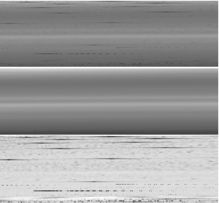
Figure 1: Examples (from top to bottom) of the initial image of echelle orders, its 2-D continuum and normalized image.

Figure 2: Mean spectrum (the upper plot) and standard deviation $\sigma$ at the H$\beta$ and H$\gamma$ profile of Vega spectrum.

Normalization to the continuum deserves some additional comments. In order to obtain uniformly reconstructed continuum in all the spectra we applied the following technique. After the flat-fielding procedure all extracted spectral orders of individual frames were merged into new 2-D (4000x75) images where the echelle orders (75 orders in total) where consequently placed as image rows. Then, with the aid of the median and Gaussian filters, we identified and cut out all narrow spectral features in all spectral orders. Finally, ignoring the Balmer line regions we fitted all the images using 2-D cubic spline function and created 2-D continuum images. Normalized spectra were produced by the division of the initial images by their corresponding 2-D continuum images. Examples of the initial image, 2-D continuum derived from it and normalization results are presented in Fig. 1.

Our analysis showed that such a technique makes it possible to achieve a required high accuracy and stability of the continuum reconstruction in those places of the observed spectra where the spectrograph’s response function can be described by a monotonic low-order polynomial 2-D function. For the BOES the most appropriate region is from 4150 to about 5100 Å  that makes our analysis reliable at the H$\gamma$ and H$\beta$ Balmer lines. Accuracy of the continuum normalization around these lines is estimated to be approximately 0.1–0.2%. In order to illustrate this conclusion, here we present results of test observations of Vega which were carried out in different nights in the period from early March to May of 2006. It is established (Peterson et al., 2006) that this standard star has the inclination of the rotational axis $i=4.5\degr\pm 0.33\degr$. Such a small inclination minimizes the probability to detect any physical variability in the Balmer profiles of Vega’s spectrum allowing to use this star as a standard in our study. Results of the tests are presented in Fig. 2 where the upper plot illustrates mean spectrum of the star obtained by averaging the observed spectra. The lower plot is the dispersion of the result obtained as standard deviation of the individual spectra from the mean. As can be seen from the behavior of the dispersion function, all instabilities of the continuum reconstruction lie typically below $0.15-0.2$%.

Also, we would like to note that during these observations the spectrograph’s configuration has been changed many times by service requirements. Nevertheless, the response function of the spectrograph showed very good stability despite the fact of these re-configurations. Analyzing observations of another program Ap/Bp stars which do not show any significant variability of the Balmer profiles we also concluded that the response function does not change its shape for the last three years (2003-2006).

For different reasons, the stability around the other Balmer lines is not so good compared to the H$\gamma$ and H$\beta$ regions. For example, the H$\alpha$ region is characterized by the presence of a narrow slope of the response function that makes it difficult to reconstruct continuum around this line with the necessary accuracy. However, in this study we decided to include the H$\alpha$ line also as an illustration.

Taking all the above conclusions into account we searched the Balmer line profile variations using normalized spectra at the H$\alpha$, H$\beta$, and H$\gamma$ regions. For each of the spectral intervals we examined the standard deviation $\sigma$ from the mean in the profiles during full rotation cycle of the star. The standard deviations as function of wavelength are presented in Fig. 3. Analyzing spectral regions with low lines density we found that the standard deviation due to the photon noise and inaccuracies in the spectra processing lie below the level of 0.3%. Any deviation above this value indicates the presence of significant intrinsic variability of Balmer line profiles.

Figure 3: The standard deviation $\sigma$ at the H$\alpha$, H$\beta$ and H$\gamma$. The photon noise background of $\sigma\approx 0.3$% is subtracted.

The standard deviations at the H$\beta$ and H$\gamma$ reveal the characteristic fingerprint first described by Kroll, (1989) as the impact of the Lorentz force: the amplitude rises in the wings and drops to the line center. This picture is less clear for the H$\alpha$ line due to the above reasons and strong distortion of the profile by the telluric molecular absorptions. (Here we note that the spectra obtained at different dates on the time base of about one year are strongly Doppler-shifted relative to each other due to the Earth’s movement. In this connection our study requires rebinding the spectra to the rest wavelengths and, as a result, all the telluric lines become randomly shifted in the individual rebined spectra that strongly complicates analysis of the H$\alpha$ profile). Nevertheless, the effect is seen in the red wing of the line (see Fig. 3).

The narrow features in the standard deviations (H$\beta$ and H$\gamma$ lines, Fig. 3) come from metal lines located in wings of the hydrogen line profiles. Strong variability of these lines indicates the presence of an inhomogeneous surface distribution of corresponding chemical abundances. This distorting factor contributes to an additional noise but it can be isolated and separated from the broad spectral changes in the hydrogen lines.

3 Model

3.1 General equations and approximations

In order to model the found variation of the Balmer line profiles we assume that this variability is caused by the Lorentz force and follow approaches outlined by Valyavin et al., (2004).

In the presence of the Lorentz force term the hydrostatic equation reads:

$$\@vec{\nabla}P_{\rm total}=\rho\@vec{g}+\@vec{f}_{\rm L},$$ (2)

and

$$\@vec{f}_{\rm L}=\frac{1}{c}\@vec{j}\times\@vec{B},$$ (3)

where $P_{\rm total}=P_{\rm gas}+P_{\rm rad}$ denotes the total pressure, $P_{\rm gas}$ and $P_{\rm rad}$ are the gas and radiation field pressures respectively, $\rho$ is the gas density, $\@vec{g}$ is the surface gravity, $\@vec{j}$ and $\@vec{B}$ are the surface currents and magnetic field vector respectively, and $c$ is the speed of light. The electric currents are determined using the Ohm’s law:

$$\@vec{j}=\lambda\@vec{E}_{\rm\parallel}+\lambda_{\rm\perp}\@vec{E}_{\rm\perp}+\lambda_{\rm H}\frac{\@vec{B}\times\@vec{E}_{\rm\perp}}{B},$$ (4)

where $\@vec{E}_{\rm\parallel}$ and $\@vec{E}_{\rm\perp}$ are electric field components directed along and across magnetic field lines respectively, $\lambda$ is the electric conductivity in the absence of the magnetic field, $\lambda_{\rm\perp}$ is the electric conductivity across the magnetic field lines and $\lambda_{\rm H}$ is the Hall’s conductivity.

To simplify solution of the problem, we consider poloidal surface magnetic field geometry. The non-force-free term giving rise in the Lorentz force is described via the induced electric field ($e.m.f.$). This configuration can be justified in the context of the magnetic field evolution. For example, distortion of initially force-free configuration of the magnetic field and respective distribution of the electric field over the stellar surface may be produced by the global field decay/generation or by any other, more complicated scenario related, for instance, to generation of internal toroidal fields by differential rotation etc. In the present study we do not consider these details and generalize the problem making no assumption about the origin of the Lorentz force. Following the approach developed in previous studies and taking into account the fact that the surface magnetic field of the majority of CP stars may approximately be described by low-order axisymmetric poloidal fields, we restrict our model considering only azimuthal geometry of the induced electric field. In this case the equations introduced above can be implemented in a 1-D stellar model atmosphere code.

Finally, the complete set of assumptions used in our modelling can be summarized as follows:

1. The stellar surface magnetic field is axisymmetric and is dominated by dipolar or dipole+quadrupolar component in all atmospheric layers.

2. The induced $e.m.f.$  has only an azimuthal component, similar to that described by Wrubel, (1952), who considered decay of the global stellar magnetic field. In this case the distribution of the surface electric currents can be expressed by the Legendre polynomials $P^{1}_{n}(\mu)$, where $n=1$ for dipole, $n=2$ for quadrupole, etc., and $\mu=\cos\theta$ is the cosine of the co-latitude angle $\theta$ which is counted in the coordinate system connected to the symmetry axis of the magnetic field.

3. The atmospheric layers are assumed to be in static equilibrium and no horizontal motions are present.

4. Stellar rotation, Hall’s currents, ambipolar diffusion and other dynamical processes are neglected.

Taking into account these approximations and substituting Eq. (3) and Eq. (4) into Eq. (2), we can write the hydrostatic equation in the following form

$$\frac{\partial P_{\rm total}}{\partial r}=-\rho g\pm\frac{1}{c}\lambda_{\rm\perp}\sum_{n}c_{n}P^{1}_{n}(\mu)\sum_{n}B^{(n)}_{\rm\theta}.$$ (5)

Obtaining this equation we used the superposition principle for field vectors and the solution of Maxwell equations for each of the multipolar components following Wrubel, (1952). We also suppose that $\@vec{E}\perp\@vec{B}$. Here $c_{n}$ represents the effective electric field generated by the $n$-th magnetic field component at the stellar magnetic equator and $B_{\rm\theta}$ is the horizontal field component. The signs “+” and “–” refer to the outward and inward directed Lorentz forces, respectively. Equation (5) can be solved if the plasma conductivity $\lambda_{\rm\perp}$ is known.

We note that the values of $c_{n}$ are free parameters to be found by using our model. These values represent the fundamental characteristics which can be used for building self-consistent models of the global stellar magnetic field geometry and its evolution. Thus, an indirect measurement of these parameters via the study of the Lorentz force is of fundamental importance for understanding the stellar magnetism.

3.2 Calculation of plasma conductivity

Calculation of the electric conductivity $\lambda_{\rm\perp}$ can be carried out using the Lorentz collision model where only binary collisions between particles are allowed. The detailed description and basic relationships of this approach is given in Valyavin et al., (2004). Improving the latter work, here we calculate the electric conductivity including all available charged particles. The precise calculations require direct evaluation of the effective stopping force acting between two charged particles of types $k$ (background particle) and $i$ (test particle):

$$F_{\rm eff}^{(ik)}=\frac{4\pi(Z_{i}e)^{2}(Z_{k}e)^{2}n_{k}\ln\Lambda}{Mv_{k,\rm T}^{2}}f_{ik}\left(\frac{v_{i}}{v_{k,\rm T}}\right).$$ (6)

Here $n_{k}$ and $v_{k,\rm T}$ are the concentration and the most probable thermal velocity of particles of type $k$, $Z_{i}$ and $Z_{k}$ are charges of the particles, $M$ is the reduced mass and $\ln\Lambda$ is the classical Coulomb logarithm. The Chandrasekhar function $f(x)$ has the following form (Chandrasekhar, 1942):

$$f(x)=\frac{2}{\sqrt{\pi}}x^{-2}\left[\int_{0}^{x}e^{-x^{2}}dx-xe^{-x^{2}}\right].$$ (7)

In the case of the interaction between charged and neutral particles we use the elastic collision cross-sections,

$$\sigma_{k}=\pi a_{0}^{2}\left(\frac{m_{k}}{m_{\rm p}}\right)^{-2/3},$$ (8)

where $a_{0}$ is the Bohr radius and $m_{\rm p}$ is the proton mass.

Generally, at the uppermost atmospheric layers where the cyclotron frequency of the conducting particles is much higher than their mean free-path times, effects of magnetoresistivity on $\lambda_{\rm\perp}$ redirect induced horizontal electric currents into Hall’s currents (see Valyavin et al., 2004) which are ignored in our model. In the deepest layers, the effects of the magnetic field influence on the conductivity become negligible and electric currents can be described by ordinary Ohm’s law for the non-magnetic case. In the intermediate atmospheric layers, however, the situation becomes more complicated. Under the influence of horizontal magnetic field, the contribution of ionized particles to the conductivity is strongly stratified by the magnetic field that produces the bimodal shape of the Lorentz force term (Valyavin et al., 2004).

Computations of the electric conductivity under the aforementioned assumptions enables us to present the solution via unknown induced $e.m.f.$  ($c_{n}$) and magnetic field determined from observations. A preliminary analysis (see also Valyavin et al., 2004) showed that amplitudes of the pressure-temperature modification with the Lorentz force depend mainly on the induced $e.m.f.$ Magnetic field strength also influences the amplitudes but mainly affects the positions of the perturbed bimodal area on the Rosseland optical depth scale. For the very small magnetic fields the perturbation of the atmosphere is limited to small Rosseland optical depths above the region where the wings of the Balmer lines form. Increasing the magnetic field strength shifts the perturbation toward the deeper regions, which contribute to the formation of hydrogen lines. In this process the two maxima of the bimodal atmospheric perturbations pass one after another through the zone of Balmer line formation, giving rise to maximum perturbations to the Balmer line formation around horizontal local magnetic field $B_{\theta}$ of 400–500 G and 10000 G with a significant gap between $B_{\theta}=1$ kG and $6$ kG. In terms of global, nearly dipolar magnetic fields these areas of the most effective contribution of the horizontal magnetic field to the Balmer line formation correspond to approximately 1 kG and 20 kG magnetic stars. Taking into account that the majority of magnetic stars have magnetic fields weaker than 10 kG we predict that the maximum amplitudes of the Balmer line variation due to the Lorentz force are expected to be among magnetic Ap/Bp stars with magnetic fields between 0.4 kG and 1–2 kG. The $\theta$ Aur  is one of such stars.

3.3 Model atmospheres with Lorentz force

Our calculations were carried out with the stellar model atmosphere code LLmodels  developed by Shulyak et al., (2004). The code is based on the modified ATLAS9  (Kurucz, 1993a ) and ATLAS12  (Kurucz, 1993b ) subroutines as well as on the spectrum synthesis package described by Tsymbal, (1996). LLmodels  is written in Fortran 90 and uses the following general approximations (which are typical for many 1-D model atmosphere tools):

• the plane-parallel geometry is assumed;

• the Local Thermodynamic Equilibrium (LTE) is used to calculate the atomic level populations for all chemical species;

• the stellar atmosphere is assumed to be in a hydrostatic equilibrium;

• the radiative equilibrium condition is fulfilled.

The code incorporates the so-called line-by-line (LL) method of the bound-bound opacity calculations (Shulyak et al., 2004). This technique allows us to account for individual stellar abundance pattern, which is important in the present study of $\theta$ Aur  because this star shows non-solar abundances and an inhomogeneous horizontal distribution of some chemical elements. In this case accurate treatment of lines opacity in model atmospheres is needed to ensure correct calculation of model structures with individual abundance patterns.

The new module was written to compute electric conductivity and magnetic pressure. Since the effective gravity is a function of atmospheric depth, additional changes in the solution of the hydrostatic equation and in the mass correction routines were made. The hydrostatic equation is solved and presented in terms of monochromatic optical depth scale $\tau_{\rm 5000}$ as an independent variable. At each iteration the code calculates electric conductivity in all atmospheric layers using all available charged and neutral plasma particles. The conductivity is then used to evaluate magnetic contribution to the effective gravity and to execute mass correction procedure.

As can be seen from Eq. (5), in the case of the outward directed Lorentz force, there is some critical value of $c_{n}$ which may produce unstable solution. Such models can not be considered in the hydrostatic equilibrium approximation introduced above and were assumed to be non-physical in our calculations. Thus, for each set of models, we adopted $c_{n}$ values as to ensure static equilibrium.

In addition, the following calculation settings have been used: the atmosphere is sliced into 72 layers equally spaced along the Rosseland optical scale height $\tau_{\rm Ross}$, from ${\tau_{\rm Ross}=-6.875}$ to ${\tau_{\rm Ross}=2.0}$. The number of frequency points used for the flux integration procedure was 495 000 in the 500–50 000 Å  spectral region. The initial atomic line list taken from VALD (Vienna Atomic Line Database) (Piskunov et al., 1995; Kupka et al., 1999) contains information about 21.6 million atomic lines, including lines originating from the predicted energy levels. This line list was used as an input for the preselection procedure in the LLmodels  code. We adopted the selection threshold $\ell_{\rm\nu}/\alpha_{\rm\nu}\geqslant 1$%, where $\alpha_{\rm\nu}$ and $\ell_{\rm\nu}$ are the continuum and line absorption coefficients at the given frequency $\rm\nu$. The preselection enabled us to reduce the total number of lines used for the line opacity calculations to about 525 000.

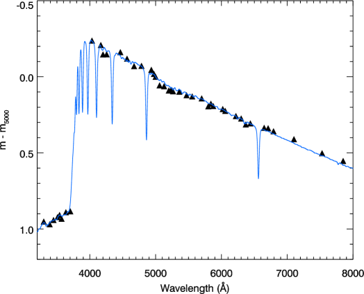
Figure 4: Comparison of the observed (symbols) and computed (solid line) energy distribution of $\theta$ Aur. Theoretical model corresponds to $T_{\rm eff}=10\,400$ K, $\log g=3.6$, and has been convolved with a $FWHM$ = 20 Å  Gaussian filter.

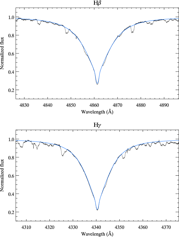
Figure 5: Comparison of the observed and computed H$\beta$ (upper panel) and H$\gamma$ (lower panel) profiles. Thick line shows observations at phase 0.995, thin line corresponds to synthetic spectra.

4 Results

4.1 Model atmosphere parameters of $\theta$ Aur

The model atmosphere parameters, $\log g$ and $T_{\rm eff}$, were determined using spectrophotometric energy distribution (Adelman et al., 1987) and theoretical fit of the H$\beta$ and H$\gamma$ line profiles. For this purpose we have chosen observations at phase 0.995 (polar region) where the influence of the Lorentz force is small and the stellar atmosphere is expected to be close to the standard non-magnetic model structure. The chemical composition as well as the projected rotational velocity $v\sin i=55$ km s^-1 were taken from Kuschnig, (1998), who used multi-element Doppler Imaging technique to derive surface maps for eight elements in $\theta$ Aur. Table 2 gives abundance patterns for four representative rotation phases.

Table 2: The surface-averaged abundances ($\log N/N_{\rm total}$) of $\theta$ Aur  for the four rotation phases (Kuschnig, 1998) and averaged over the whole stellar surface (last column).

Element	0.00	0.25	0.50	0.75	average
He	-2.32	-2.32	-2.40	-2.32	-2.34
Mg	-5.28	-5.27	-5.35	-5.50	-5.35
Si	-3.35	-3.27	-3.09	-3.22	-3.23
Ti	-7.52	-7.61	-7.67	-7.61	-7.60
Cr	-5.14	-5.35	-4.99	-4.75	-5.06
Mn	-5.50	-5.64	-5.49	-5.34	-5.49
Fe	-3.86	-3.83	-3.63	-3.69	-3.75
Sr	-8.43	-8.43	-8.36	-8.19	-8.35

Synthetic Balmer line profiles were calculated using the Synth program (Piskunov, 1992). The program incorporates recent improvements in the treatment of the hydrogen line opacity (Barklem et al., 2000). The stellar energy distribution and Balmer lines are best approximated with the following parameters: $T_{\rm eff}=10\,400\pm 300$ K, $\log g=3.6\pm 0.05$. Note, that such a high accuracy of the determined parameters is just an internal accuracy obtained from our technique which we used to fit the data. Real parameters may be slightly different from the obtained ones due to various systematic error sources, but this does not play a significant role in our study. Comparison of the observations and model predictions are presented in Fig. 4 and Fig. 5. Fundamental parameters of $\theta$ Aur  suggest that this star is significantly evolved from the ZAMS. From the comparison with theoretical evolutionary tracks Kochukhov & Bagnulo, (2006) find $\theta$ Aur  to be at the very end of its main sequence life.

Recent studies by Kochukhov et al., (2005) and Khan & Shulyak, 2006a ; Khan & Shulyak, 2006b showed that the effects of Zeeman splitting and polarized radiative transfer on model atmosphere structure and shapes of hydrogen line profiles are less than 0.1% for magnetic field intensities around 1 kG and thus can be safely neglected in the present investigation.

4.2 Magnetic field geometry

To calculate the Lorentz force effects it is essential to specify the magnetic field geometry (see Eq. (5)). The first longitudinal magnetic field measurements were obtained for $\theta$ Aur  by Borra & Landstreet, (1980) using H$\beta$ photopolarimetric technique. The authors observed a smooth single-wave $\langle B_{\rm z}\rangle$ variation with rotation phase and concluded that it is probably caused by a dipole inclined to the rotation axis of the star. Wade et al., (2000) presented high-precision longitudinal field measurements of this star. They confirmed and improved results of Borra & Landstreet, (1980). In particular, deviation of the $\langle B_{\rm z}\rangle$ variation from the purely sinusoidal magnetic curve has been found (see Fig. 12 in Wade et al., 2000).

Following these works, we have approximated magnetic field topology of $\theta$ Aur by a combination of the dipole and axisymmetric quadrupole magnetic components. We have also assumed that the symmetry axes of the dipole and quadrupole magnetic fields are parallel. Thus, the model parameters include the polar strength of the dipolar component $B_{\rm d}$, relative contribution of the quadrupole field $B_{\rm q}/B_{\rm d}$, magnetic obliquity $\beta$, and inclination angle $i$ of the stellar rotation axis with respect to the line of sight. The last parameter is best estimated independently, from the usual oblique rotator relation connecting stellar radius, rotation period and $v\sin i$. Hipparcos parallax $\pi=18.83\pm 0.81$ mas and $T_{\rm eff}=10\,400\pm 300$ K yield $R=5.1\pm 0.4\,R_{\odot}$. This leads to $i=51\degr\pm 6\degr$, which is in good agreement with $i=$ 50°–60° derived in Doppler imaging studies (Rice & Wehlau, 1991; Kuschnig, 1998).

The remaining free parameters of our model for the magnetic field geometry were determined with the least-squares fit of the observed $\langle B_{\rm z}\rangle$ variation (Borra & Landstreet, 1980; Wade et al., 2000). We have examined “positive” (quadrupolar field has two positive and one negative poles) and “negative” (the two negative and one positive poles) quadrupolar field configurations. We found that the lowest $\chi^{2}_{\nu}\equiv\chi^{2}/\nu$ corresponds to the negative quadrupolar configuration with $B_{\rm q}/B_{\rm d}\approx-2$ ($\chi^{2}_{\nu}=1.14$, $B_{\rm d}=1.4$ kG, $\beta=78\degr$), while the purely dipole model gives $\chi^{2}_{\nu}=2$ ($B_{\rm d}=1.3$ kG, $\beta=73\degr$).

4.3 Effects of horizontal abundance distribution

In order to distinguish effects of the magnetic pressure from the ones of the abundance distribution, we calculated model atmospheres for each of the four representative phases using individual abundances from Table 2. The synthetic profiles of the hydrogen lines as well as the standard deviation of the profiles due to the variable chemical abundances at the listed phases were then calculated. The results are presented in Fig. 6. As one can see, effects due to a non-uniform abundance distribution are totally different from the observed one: the strongest variability occurs in the line core whereas the line wings are not affected much. This allows us to conclude that the chemical spots do not lead to the observed Balmer line variations. This fact is in concordance with the results obtained by Kroll, (1989), who showed that the found shape of the Balmer line variability can not be reproduced by metallicity or temperature variations, but can be considered in the frame of changes in the pressure structure of the stellar atmosphere. Finally, the average abundances from Table 2 (last column) were used in the rest of model atmosphere calculations.

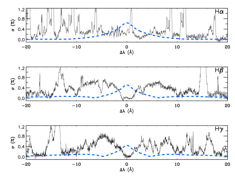
Figure 6: The standard deviation $\sigma$ at the H$\alpha$, H$\beta$ and H$\gamma$ lines. Observations are shown by solid lines. The dashed lines illustrate variability due to the horizontal abundance inhomogeneities.

4.4 The Lorentz force

In order to fit the observed variations of the line profiles, both the inward and outward directed Lorentz forces were examined through the model atmosphere calculations. The actual magnetic input parameters of computations with LLmodels  code include the sign of the Lorentz force, magnetic field modulus $B$, and the product of two sums $\sum c_{n}P^{1}_{n}\sum B^{(n)}_{\rm\theta}$. Following the procedure described by Valyavin et al., (2004), we take the latter two parameters to be disk-averaged at the individual rotation phases. We used this simplified procedure because a direct integration of the model over the stellar surface is a very time-consuming process under our approaches. The most general and precise way to produce a disk-integrated model spectrum is to

• calculate (for given $c_{n}$ and the polar strength $B^{(n)}_{\rm p}$) a number of local model atmospheres and synthetic spectra for all surface areas from the magnetic equator to the pole,

• integrate the local spectra over the visible stellar hemisphere for a set of rotational phases and given orientation of the stellar rotational and magnetic axis.

At the present stage of our studies we are not yet ready to carry out such computations. Thus, our basic modelling strategy is to replace the flux from the disk-integrated model which should be computed for each observed phase with the flux from a single atmosphere model from LLmodels, with parameters which represent approximately the disk-averaged means.

On the other hand, our additional study revealed that even the strongest possible intensities of the Lorentz force do not change significantly the limb darkening in computations with the magnetic model compared to the non-magnetic one. Therefore, for the first investigation we used the above simplified approach. This approximate method essentially assumes linear response of the properties of magnetic atmospheres to changes in the input parameters.

Finally, the Lorentz force in the cases of dipole and quadrupole magnetic field geometries can be written as

$$\frac{\partial P_{\rm total}}{\partial r}=-\rho g\pm\frac{1}{c}\langle\lambda_{\rm\perp}\rangle c_{1}\left\langle\left(P^{1}_{1}(\mu)+\frac{c_{2}}{c_{1}}P^{1}_{2}(\mu)\right)\left(B^{(1)}_{\rm\theta}+B^{(2)}_{\rm\theta}\right)\right\rangle,$$ (9)

where braces mean the disk-averaging operation ($\langle\lambda_{\rm\perp}\rangle$ here means the “effective” conductivity calculated with the magnetic field strength averaged over the stellar disc). Equation (9) can be written in a simplified form by introducing the effective acceleration $g_{\rm eff}$ as a sum of gravitational and magnetic accelerations so that

$$\frac{\partial P_{\rm total}}{\partial r}=-\rho g_{\rm eff}.$$ (10)

Results of the disk-averaging procedure of the magnetic parameters are illustrated in Table 3 where we adopted $B_{\rm q}/B_{\rm d}=0.0$ (dipole) and $-2.0$ (dipole+quadrupole). Several sets of models with the outward and inward directed Lorentz force and $B_{\rm q}/B_{\rm d}$ ranging from 0.5 to $-2.0$ with a step of 0.5 were then calculated. The best fit to the shape of the observed hydrogen line variation was finally found for the following parameters: $c_{2}/c_{1}=2.5$ and $B_{\rm q}/B_{\rm d}=-2.0$.

Numerical tests showed that, in order to reproduce the amplitudes of the observed standard deviations due to the profile variations in case of the inward directed Lorentz force, the effective electric field should be $c_{1}=2\times 10^{-10}$ CGS units for the dipolar configuration and $c_{1}=1\times 10^{-10}$ CGS units for the dipole+quadrupole model. In case of the outward directed Lorentz force these values should be $c_{1}=3.5\times 10^{-11}$ CGS units and $c_{1}=1\times 11^{-11}$ CGS units, respectively. Increasing $c_{1}$ further leads to unstable solution. This occurs for both inward and outward directed Lorentz forces. In the latter case this means that magnetic force directed outwards becomes stronger than the gravitational force, numerically forcing $P_{\rm gas}<0$. For example, the critical value of the effective electric field is $c_{1}\approx 2\times 10^{-11}$ CGS units for dipole+quadrupole configuration. In spite of the fact that inward directed Lorentz force increases pressure of stellar plasma, the enormous increase of $c_{1}$ causes a failure of some numerical algorithms implemented in the model atmosphere code (mainly hydrostatic equation). This also causes numerical problems with the interpolation of partition functions for some elements. The estimated critical value for inward directed force is $c_{1}>2\times 10^{-10}$ CGS units for dipole+quadrupole configuration.

Table 3: Results of the surface averaging procedure for the dipole and dipole+quadrupole ($B_{\rm q}/B_{\rm d}=-2.0$, $c_{2}/c_{1}=2.5$) magnetic field configurations. Field strengths are given in Gauss.

Rotation	dipole		dipole+quadrupole
Phase	$\langle B\rangle$	$\langle P^{1}_{1}B_{\rm\theta}\rangle$	$\langle\sum B^{(n)}\rangle$	$\langle\sum\frac{c_{n}}{c_{1}}P^{1}_{n}\cdot\sum B^{(n)}_{\rm\theta}\rangle$
0.056	856	436	2158	-2652
0.061	854	438	2147	-2636
0.091	842	449	2077	-2533
0.111	833	458	2016	-2449
0.121	829	463	1982	-2406
0.250	812	480	1530	-1913
0.331	863	429	1332	-1836
0.356	886	406	1289	-1878
0.377	905	388	1261	-1931
0.393	920	373	1240	-1987
0.456	965	331	1188	-2198
0.496	975	321	1177	-2256
0.562	955	340	1199	-2145
0.681	852	439	1358	-1827
0.775	806	485	1613	-1989
0.837	813	479	1833	-2224
0.861	821	470	1921	-2329
0.936	853	439	2142	-2627
0.950	858	434	2169	-2668
0.995	865	427	2210	-2734

Figure 7: Run of the effective acceleration with Rosseland optical depth in the atmosphere of $\theta$ Aur obtained for all 20 phases of the star’s rotation. The calculations were carried out for inward directed (upper plot) and outward directed (lower plot) Lorentz force for dipole+quadrupole magnetic field configuration.

Figure 7 illustrates resulting dependence of $g_{\rm eff}$ on the Rosseland optical depth in the atmosphere of $\theta$ Aur ($B_{\rm q}/B_{\rm d}=-2,c_{2}/c_{1}=2.5$). The formation region of the central parts of Balmer lines ($\log\tau_{\rm Ross}<-1$ and above) demonstrates strong changes in the effective gravity during rotation that results in the Balmer line variations. Examination of the purely dipolar model gives similar results.

As follows from Eq. (9), the resulting disc-averaged atmospheric perturbations due to the Lorentz force depend on the competition between the effective electric conductivity $\langle\lambda_{\rm\perp}\rangle$ and the product $\langle\sum\frac{c_{n}}{c_{1}}P^{1}_{n}\cdot\sum B^{(n)}_{\rm\theta}\rangle$ averaged over the disc. The electric conductivity $\langle\lambda_{\rm\perp}\rangle$ across the magnetic field lines of force is reduced in comparison to the non-magnetic conductivity by the full disc-averaged magnetic field $\langle\sum B^{(n)}\rangle$ (the magnetoresistivity effect, see $\S$ 2 in Pikelner, (1966); Cowling, (1957); Schluter, (1950)). In our dipolar magnetic field model $\langle B\rangle$ (and the magnetoresistivity as a result) varies with an amplitude of about 10% about the average value, which is almost twice smaller than the variation of the weighted-average of the horizontal magnetic field (see Table 3). Therefore, in case of the dipolar geometry, variation of the Balmer lines is produced mainly by phase variation of the horizontal magnetic field. In the dipole+quadrupole configuration however, the variation of conductivity also plays noticeable role due to significant rotational modulation of $\langle\sum B^{(n)}\rangle$ (Table 3), which explains the influence of magnetoresistivity on the Balmer line variations for this geometry.

4.5 Comparison with the observations

We compared observations and theoretical predictions for each of the rotation phases. To minimize effects of systematic errors in the modelling procedure, we have examined residual theoretical and observed Balmer lines, which are obtained by subtracting a spectrum at a reference phase ($\phi=0.056$ where the Balmer profiles have the largest widths) from all the other spectra. Figures 8, 9 and 10 illustrate residual H$\alpha$, H$\beta$ and H$\gamma$ line profiles for each of the observed rotation phases. The positive sign of the residuals implies that the lines at the current phase are narrower than those obtained at the reference phase. Here we present only those calculations, which are able to reproduce the observed positive deviations with satisfactory accuracy. This is achieved for the purely dipolar geometry of the magnetic field with the inward directed Lorentz force (dotted lines in the figures) and by examination of the dipole+quadrupole geometry with the outward directed force (thick solid lines).

The most noticeable effect is seen at phases between $\phi\leavevmode\nobreak\ =\leavevmode\nobreak\ 0.250$ and $\phi=0.6$. However, both models fit the data only in the phase region between $\phi=0.45$ and $\phi=0.6$. We attribute this disagreement to our assumption of the axisymmetric magnetic field geometry (in reality the field can be decentered or distorted). Despite this discrepancy we suppose that our model reproduces general phase dependence found in observations.

Comparing results of the fit obtained from both models we conclude that observations are better reproduced in the case of the outward directed Lorentz force for the dipole+quadrupole magnetic field geometry. As can be seen from Fig. 9, 10 the inward directed force gives too wide line wings and is unable to describe the line cores of the observed residual spectra. In contrast, the outward directed Lorentz force shows better agreement with observations. Such a difference between the two models results from the fact that at the upper atmospheric layers of the Balmer line formation regions the inward directed Lorentz force changes the pressure-temperature balance more effectively than the outward directed one (see Fig. 7). Increasing $g_{\rm eff}$, the inward directed Lorentz force makes the Balmer line profiles non-realistically wider than the observed ones. This makes the outward directed magnetic force more preferable in our analysis.

The best fit obtained with $B_{\rm q}/B_{\rm d}=-2.0$ and $c_{2}/c_{1}=2.5$ agrees with the longitudinal field modelling results. The outcome of the H$\gamma$ line profile analysis (Fig. 10) is in satisfactory agreement with the H$\beta$ line modelling. In the case of the H$\alpha$ line (Fig. 8) it is difficult to distinguish predictions of the two models.

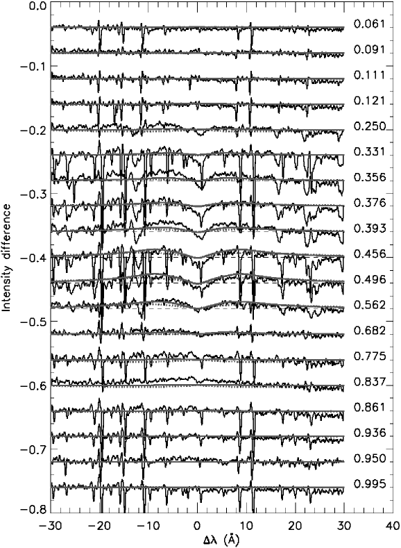
Figure 8: Residual profiles of the H$\alpha$ line for each of the observed phase relative to the phase 0.056. Thin solid lines are observations, dotted lines are theoretical profiles calculated for the dipole magnetic field configuration (inward directed Lorentz force), thick solid lines are profiles calculated for the dipole+quadrupole magnetic field configuration with $B_{\rm q}/B_{\rm d}=-2.0$ and $c_{2}/c_{1}=2.5$ (outward directed Lorentz force). The residual spectra for consecutive phases are shifted in the vertical direction. The thin dashed line gives zero level for each spectrum.

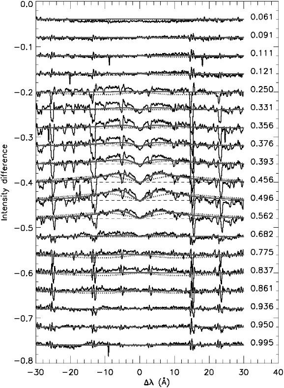
Figure 9: Same as Fig. 8 but for H$\beta$ line.

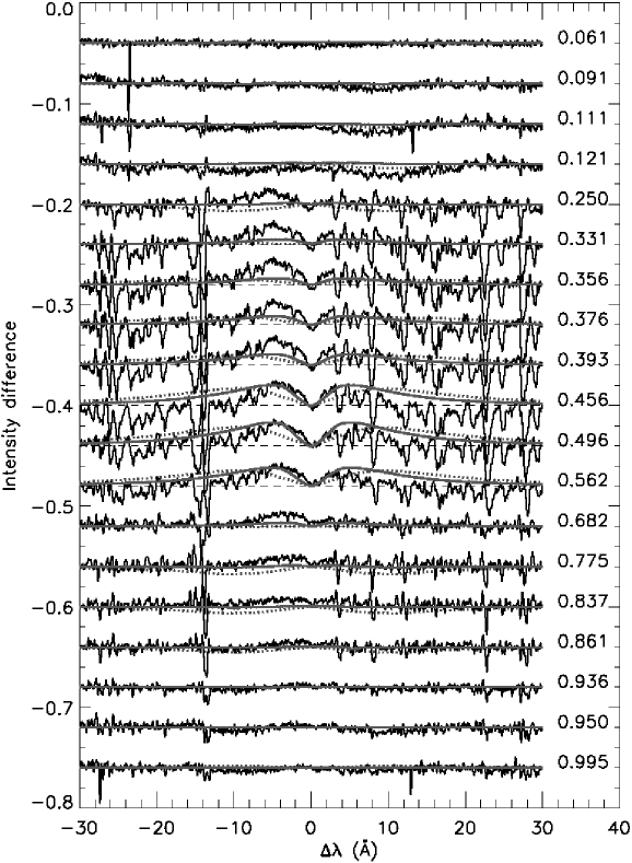
Figure 10: Same as Fig. 8 but for H$\gamma$ line.

Now, before general discussion, we would like to clarify some points in the above modelling approaches. The observed changes in Stark profiles of the Balmer lines demonstrate monotonic single-wave variation during full rotation cycle of $\theta$ Aur. Originally, however, we expected another picture of the variations due to predicted dominant dipolar component of the magnetic field in this star. According to previous studies (Valyavin et al., 2004, and references therein) we expected that if a magnetic star with centered dipolar field shows the observer both positive and negative parts of its magnetosphere during rotation (that takes place in $\theta$ Aur), the hydrogen lines should demonstrate double-wave variations during full rotation cycle. To resolve this difficulty, we have included the quadrupole component, which is still not well-established for $\theta$ Aur, but is plausible for the reasons mentioned above. In the contrast to the purely dipolar magnetic field, the combination of dipole+quadrupole enables us to derive a satisfactory fit to the observed behavior of the Balmer line variations. As follows from Table 3, we are able to obtain a configuration of the dipole+quadrupole magnetic field for which the maximum visible horizontal component is located at those phase points where the varying longitudinal magnetic field exhibits extremum (not at the crossover). Such a configuration gives the single-wave variation of the Lorentz force and reproduces our observations.

Another important point is related to different orientations of the Lorentz force obtained for the two examined geometries of the magnetic field. For both geometries with the opposite-oriented Lorentz force the sign of the resulting Balmer line residual variations is unchanged at the extremal point of the phase curve ($\phi\approx 0.5$). In this connection we note again (see above), that the Stark widths variations in the purely dipolar model are mainly produced by the horizontal magnetic field that provides the minimum inward directed Lorentz force at this phase due to the minimum of visible horizontal component (see Table 3). The Stark widths of the lines are reduced at this phase in comparison to the other phases. In contrast, the dipole+quadrupole geometry of the magnetic field provides significant horizontal component at this point and minimum magnetoresistivity that results in the maximum outward directed magnetic force term. As a result, the Stark widths of the Balmer lines are also reduced at this phase relatively to all the other phases of the stellar rotation even implementing the opposite orientation of the Lorentz force.

Despite the fact that a fairly good agreement with observations is obtained, we do not claim that our geometric fit is absolutely correct. For example, our assumption about essentially poloidal centered magnetic field may be wrong. Intuitively we may assume, that decentered dipole may also produce the Balmer line profile variations which can be similar to the observed ones. Besides, we do not exclude the presence of more complicated dynamical, non-evolutionary processes such as meridional circulation which can also produce similar observable features. The problem is too complicated, and the answer about the true model parameters (also about the true nature of the Lorentz force) can be obtained only when the exact geometry of the surface field in $\theta$ Aur will be established. In this study we only demonstrate that the observations can be described with simple geometrical approaches about magnetic field and induced electric currents. We therefore conclude that the main achievement of this paper is not our explanation of the behavior of the phase-resolved Balmer line profiles, but our argumentations for the presence of the detectable Lorentz force in the atmosphere of $\theta$ Aur.

5 Conclusions

With the aim to probe the presence of the Lorentz force in atmospheres of magnetic CP stars, we have acquired new high-precision spectral observations for one of the bright magnetic stars, $\theta$ Aur. The hydrogen line profile variations are investigated using high-resolution spectra covering the full rotation cycle of the star. We have detected and studied variability of the Stark-broadened profiles of H$\alpha$, H$\beta$, and H$\gamma$. Several evidences for the presence of significant Lorentz force in atmosphere of $\theta$ Aur are found:

• The characteristic shape of the variation during full rotation cycle of the star corresponds to those described by Kroll, (1989) and other authors (Valyavin et al., 2004, and references therein) as a result of an impact of a substantial Lorentz force.

• Numerical calculations of the model atmospheres with individual abundances demonstrate that the surface chemical spots can not produce the observed variability of the hydrogen line profiles of $\theta$ Aur.

• Our model shows good agreement with the observations if the outward directed magnetic force is applied assuming the dipole+quadrupole magnetic field configuration with the induced effective equatorial electric field of $c_{1}=1\times 10^{-11}$ CGS units.

• The dipole+quadrupole magnetic model with the quadrupolar strength twice stronger than the dipolar one reproduces behavior of the phase-resolved H$\beta$ and H$\gamma$ spectra.

6 Discussion

In the above considerations we did not examine any mechanisms of the magnetic force generation. We have restricted ourselves to the purely phenomenological and geometrical description of the problem. Let us finally discuss physical processes which could create the Lorentz force in the atmospheres of magnetic CP stars.

6.1 Secular evolution of the global magnetic field

It is well known that any variation of the global stellar magnetic field (related, for instance, to a global field decay) leads to the development of the induced electric currents in conductive atmospheric layers. The Lorentz force, which appears as a result of the interaction between the magnetic field and electric currents, may affect the atmospheric structure and influence the formation of spectral lines causing their rotational variability. The sign of the observed Lorentz force (outward or inward directed) is also found to be important. For example, following Wrubel, (1952), who was the first to present numerical calculations of the decay of poloidal interior magnetic field, the decay-induced electric field $E_{\rm\phi}$ have essentially azimuthal form:

$$E_{\rm\phi}\sim g(r)P^{1}_{n}(\mu),$$ (11)

where $g(r)$ is a scalar radial function of a distance $r$ from stellar center ($r=[0,R_{\star}]$). Considering only the dipole component, the induced currents do not change sign at the stellar surface, achieving maximum strength at the magnetic equator (where the magnetic field lines of force is horizontal) and vanishing at the magnetic poles ($\theta=0\degr,180\degr$). In this case the Lorentz force corresponds to the case of the outward directed decay-induced force term at any non-polar area of the stellar surface. Therefore, determination of the sign of the Lorentz force provides an important constraint which is able to restrict direction of the field evolution.

According to Landstreet, (1987), who also considered a decay of an essentially dipolar fossil magnetic field, we should not expect any signatures of the Lorenz force in atmospheres of CP stars. In his model magnetic field has dipolar geometry throughout a magnetic star and electric field induced at the equator can be approximated with the following expression:

$$E_{\rm eq}\sim\frac{R_{\rm\star}B_{\rm eq}}{ct},$$ (12)

where ${R_{\rm\star}}$ is the stellar radius, $B_{\rm eq}$ is the strength of the dipole-like surface field at the magnetic equator and $t$ is the characteristic decay time of the magnetic field. For a typical A0 magnetic star with the surface field of 10 kG this leads to the value $E_{\rm eq}\sim 10^{-13}$ CGS, which is about 2–3 orders of magnitude smaller compared to the strength of the electric currents tested in our model calculations and inferred from the variations of hydrogen lines. The former theoretical estimate of $E_{\rm eq}$ is based on the $10^{10}$ yr characteristic decay time of nearly dipolar fields. Thus, if the observed strong electric currents in the atmosphere of $\theta$ Aur  have the evolutionary nature, we may conclude that the general concept of a slow decay of the fossil, essentially dipolar, fields requires for revision. One should examine more realistic structures of the internal fields, and this may lead to faster field evolution. As it was recently shown by Braithwaite & Spruit, (2004), dynamical stability of the global stellar magnetic fields is ensured if the interior field configuration includes both poloidal and toroidal components. Diffusive evolution of such a twisted field structure may lead to relatively rapid change of the surface field intensity. This, in turn, induces a noticeable atmospheric Lorentz force during certain periods in the star’s life. In this context advanced evolutionary stage of $\theta$ Aur is remarkable.

Thus, large amplitude of the induced electric currents may indicate that the poloidal magnetic geometry, dominating at the surface, becomes significantly distorted inside a magnetic star. Such a distortion is very likely to be related to dynamical processes of the field evolution and, possibly, interaction with the core convective zone or differential rotation.

6.2 Non-evolutionary surface effects

Generally, any global magnetic topology gives a large collection of possibilities of generation of the surface electric currents even without invoking the global magnetic field evolution. There are mechanisms which may produce significant atmospheric currents even in constant magnetic fields. For instance, Peterson & Theys, (1981) considered interaction of the horizontal component of the magnetic field with a flow of charged particles, drifting in the atmosphere under the influence of the radiation pressure. The result of such an interaction is that drifting particles acquire some horizontal velocity component. This leads to appearance of the Lorentz force which may be significant for hot stars ($T_{\rm eff}>18\,000-20\,000$ K). More recently LeBlanc et al., (1994) studied a similar physical situation in the context of ambipolar diffusion. Furthermore, interaction of the magnetic field and stellar rotation may induce dynamical processes leading to the development of additional plasma flows (such as meridional circulations) which are able to create electric currents and the Lorentz force.

We have obtained our results under the assumption that the equatorial induced electric field is constant in vertical direction. This should be close to reality if we deal with evolving global magnetic field, whose variation is small throughout the observable atmospheric layers. This assumption, however, may not be applicable if the Lorentz force is related to, for example, the ambipolar diffusion. Nevertheless, our results provide an observational test to distinguish these effects.

As it was shown by LeBlanc et al., (1994), the ambipolar diffusion is small for the weak field stars and increases in stars with the surface magnetic fields of about 10 kG and higher. It should be noted, however, that we have considered a relatively weak-field star ($B$ $\approx$ 1 kG). Moreover, the inward directed Lorentz force predicted by the ambipolar diffusion theory is not supported by our observations, as we have found a much better agreement for the outward directed magnetic force. Nevertheless, we do not claim that our approach is the only way to address the problem of the generation of the Lorentz force in the atmospheres of CP stars. Before making final conclusion about the nature of the Lorentz force found in $\theta$ Aur, alternative models should be applied to interpret our observational findings.