Reconstruction of the deceleration parameter and the equation of state of dark energy

Abstract

The new 182 gold supernova Ia data, the baryon acoustic oscillation measurement and the shift parameter determined from the Sloan Digital Sky Survey and the three-year Wilkinson Microwave Anisotropy Probe data are combined to reconstruct the dark energy equation of state parameter $w(z)$ and the deceleration parameter $q(z)$. We find that the strongest evidence of acceleration happens around the redshift $z\sim 0.2$ and the stringent constraints on $w(z)$ lie in the redshift range $z\sim 0.2-0.5$. At the sweet spot, $-1.2<w(z)<-0.6$ for the dark energy parametrization $w(z)=w_{0}+w_{a}z/(1+z)^{2}$ at the $3\sigma$ confidence level. The transition redshift $z_{t}$ when the Universe underwent the transition from deceleration to acceleration is derived to be $z_{t}=0.36^{+0.23}_{-0.08}$. The combined data is also applied to find out the geometry of the Universe, and we find that at the $3\sigma$ confidence level, $|\Omega_{k}|\lesssim 0.05$ for the simple one parameter dark energy model, and $-0.064<\Omega_{k}<0.028$ for the $\Lambda$CDM model.

I Introduction

The discovery of the accelerated expansion of the Universe by the supernova (SN) Ia observations agr98 imposes a big challenge and provides opportunities to theoretical physics. The more accurate SN Ia data riess ; astier ; riess06 , the three-year Wilkinson Microwave Anisotropy Probe (WMAP3) data wmap3 , and the Sloan Digital Sky Survey (SDSS) data sdss tell us that the Universe is almost spatially flat, and dark energy (DE) with negative pressure contributes about 72% of the matter content of the Universe. Although the existence of DE were verified by different observations, the nature of DE is still a mystery to us. For a review of DE models, one may refer to Ref. DE .

Many parametric and non-parametric model-independent methods were proposed to study the evolutions of the deceleration parameter $q(z)$, the DE density $\Omega_{DE}(z)$, the DE equation of state (EoS) $w(z)$, and the geometry of the Universe virey ; sturner ; gong06 ; astier01 ; huterer ; weller ; alam ; gong04 ; gong05 ; lind ; jbp ; par1 ; par2 ; par3 ; par4 ; par5 ; gong04a ; wang05 ; jbp05 ; nesseris6a ; berger ; sahni06 ; lihong ; yun06 ; evldh ; saini ; jbp06 ; nesseris05 ; nesseris6b . In the reconstruction of $q(z)$, it was found that the strongest evidence of acceleration happens at redshift $z\sim 0.2$ virey ; sturner ; gong06 , and the evidence of the current acceleration is not very strong sturner and model dependent gong06 . Previous studies on the reconstruction of $w(z)$ also showed that the stringent constraint on $w(z)$, or the sweet spot, happened around redshift $z\sim 0.2-0.5$ astier01 ; huterer ; weller ; alam ; gong04 ; gong05 . As Riess et al. pointed out, the use of additional parameters to reconstruct $w(z)$ does not provide a statistically significant improvement on the fit of the redshift-magnitude relation, so we discuss one- and two-parameter models only. In this work, we first use the simple two-parameter model $q(z)=1/2+(q_{1}z+q_{2})/(1+z)^{2}$ gong06 to reconstruct $q(z)$, then we use the three popular two-parameter models $w(z)=w_{0}+w_{a}z/(1+z)$ lind , $w(z)=w_{0}+w_{a}z/(1+z)^{2}$ jbp and $\Omega_{DE}=1-\Omega_{m}-A_{1}-A_{2}+A_{1}(1+z)+A_{2}(1+z)^{2}$ alam to reconstruct $w(z)$. The purpose of this work is to see if the stringent constraints on $q(z)$ and $w(z)$ still happen around $z\sim 0.2-0.5$ when we use the new 182 gold SN Ia data compiled in riess06 . The geometry of the Universe is also discussed by fitting the simple one-parameter model $w(z)=w_{0}\exp[z/(1+z)]/(1+z)$ gong05 to the combined SN Ia, SDSS and WMAP3 data.

This paper is organized as follows. In section II, we study the property of $q(z)$ by fitting the parametrization $q(z)=1/2+(q_{1}z+q_{2})/(1+z)^{2}$ to the new 182 gold SN Ia data compiled in riess06 . In section III, we apply the popular parameterizations $w(z)=w_{0}+w_{a}z/(1+z)$, $w(z)=w_{0}+w_{a}z/(1+z)^{2}$ and $\Omega_{DE}=1-\Omega_{m}-A_{1}-A_{2}+A_{1}(1+z)+A_{2}(1+z)^{2}$ to study the evolutions of DE EoS. The baryon acoustic oscillation (BAO) measurement from SDSS and the shift parameter determined from WMAP3 data combined with the new 182 gold SN Ia data are used in our analysis. In section IV, we fit the simple one-parameter representation $w(z)=w_{0}\exp[z/(1+z)]/(1+z)$ to the combined SN Ia, SDSS and WMAP3 data to obtain the geometry of the Universe. Note that the simple one-parameter model fits the observational data as well as the two-parameter models do. In section V, we conclude the paper with some discussions.

II Reconstruction of the deceleration parameter

The Hubble parameter $H(t)=\dot{a}/a$ and the deceleration parameter $q(t)=-\ddot{a}/(aH^{2})$ are related by the following equation,

$$H(z)=H_{0}\exp\left[\int^{z}_{0}[1+q(u)]d\ln(1+u)\right],$$ (1)

where the subscript 0 means the current value of the variable. If a function of $q(z)$ is given, then we can find the evolution of the Hubble parameter. For the flat $\Lambda$CDM model, $q(z)=[\Omega_{m}(1+z)^{3}-2(1-\Omega_{m})]/2[\Omega_{m}(1+z)^{3}+1-\Omega_{m}]$. In this section, we use the simple two-parameter function gong06

$$q(z)=\frac{1}{2}+\frac{q_{1}z+q_{2}}{(1+z)^{2}},$$ (2)

to reconstruct the evolution of $q(z)$. Note that $q_{0}=1/2+q_{2}$, and $dq/dz|_{z=0}=q_{1}-2q_{2}$, so the parameter $q_{2}$ gives the value of $q_{0}$. At early times, $z\gg 1$, $q(z)\rightarrow 1/2$. Substitute Eq. (2) into Eq. (1), we get

$$H(z)=H_{0}(1+z)^{3/2}\exp\left[\frac{q_{2}}{2}+\frac{q_{1}z^{2}-q_{2}}{2(1+z)^{2}}\right].$$ (3)

Since the expression for the Hubble parameter is explicit, so we can think that we are actually modelling $H(z)$ instead of $q(z)$.

The parameters $q_{1}$ and $q_{2}$ in the model are determined by minimizing

$$\chi^{2}=\sum_{i}\frac{[\mu_{obs}(z_{i})-\mu(z_{i})]^{2}}{\sigma^{2}_{i}},$$ (4)

where the extinction-corrected distance modulus $\mu(z)=5\log_{10}[d_{L}(z)/{\rm Mpc}]+25$, $\sigma_{i}$ is the total uncertainty in the SN Ia data, and the luminosity distance is

$$d_{L}(z)=(1+z)\int_{0}^{z}\frac{dz^{\prime}}{H(z^{\prime})}.$$ (5)

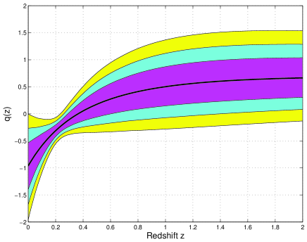
Fitting the model to the 182 gold SN Ia data, we get $\chi^{2}=156.25$, $q_{1}=1.47^{+1.89}_{-1.82}$ and $q_{2}=-1.46\pm 0.43$, here the given error is the $1\sigma$ error. For comparison, we also fit the $\Lambda$CDM model to the 182 gold SN Ia data and find that $\chi^{2}=156.16$, $\Omega_{m}=0.48^{+0.13}_{-0.15}$ and $\Omega_{k}=-0.44^{+0.43}_{-0.36}$. So the simple two-parameter model of $q(z)$ fits the SN Ia data as well as the $\Lambda$CDM model does. By using the best fitting results, we plot the evolution of $q(z)$ in Fig. 1. From Fig. 1, we see that $q(z)<0$ for $0\leq z\lesssim 0.2$ at the $3\sigma$ confidence level. This result is consistent with previous analysis by using the 157 gold SN Ia data gong06 . It is also interesting to note that the stringent constraint on $q(z)$ happens around the redshift $z\sim 0.2$. One may think perhaps there are more SN Ia data around this redshift. On the contrary, less SN Ia data is around $z=0.2$. In table 1, we list the number $N$ of SN Ia in a given redshift range for the 182 gold SN Ia data. The behavior was also found in gong06 ; astier01 ; huterer ; weller ; alam ; gong04 ; gong05 in the fitting of the EoS of DE for a variety of models. This may suggest that the behavior of DE can be better constrained in the redshift range $0.1\lesssim z\lesssim 0.6$. The sweet spot can be estimated from the covariant matrix of errors, which is the inverse of the Fisher matrix in the linear approximation astier01 ; huterer ; weller . The Fisher matrix is estimated to be $F_{11}=2.37$, $F_{12}=F_{21}=9.55$, and $F_{22}=43.9$. By choosing $\alpha_{1}=q_{1}$ and $\alpha_{2}=(F_{12}/F_{22})q_{1}+q_{2}=0.2175q_{1}+q_{2}$, the Fisher matrix becomes diagonal, $\alpha_{1}$ and $\alpha_{2}$ are uncorrelated, and the errors of $\alpha_{1}$ and $\alpha_{2}$ are $\sigma^{2}(\alpha_{1})=F_{22}/(F_{11}F_{22}-F_{12}^{2})$ and $\sigma^{2}(\alpha_{2})=F^{-1}_{22}$ dje . In terms of $\alpha_{1}$ and $\alpha_{2}$, we get

$$q(z)=\frac{1}{2}+\frac{\alpha_{1}(z-0.2175)+\alpha_{2}}{(1+z)^{2}}.$$ (6)

Now the sweet spot can be estimated from the following equation

$$\frac{2[\sigma^{2}(\alpha_{2})+\sigma^{2}(\alpha_{1})(z-0.2175)^{2}]}{1+z}=\sigma^{2}(\alpha_{1})(z-0.2175).$$ (7)

The sweet spot is estimated to be $z\simeq 0.2175$ since $\sigma^{2}(\alpha_{2})=F^{-1}_{22}\sim 0$. For a general model $w(z)=w_{1}+w_{2}f(z)$ with arbitrary function $f(z)$, the sweet spot is determined similarly from the equation $f(z)=F_{12}/F_{11}$.

Table 1: The distribution of the gold SN Ia data

$z$	$<0.1$	0.1-0.2	0.2-0.3	0.3-0.4	0.4-0.5	0.5-0.6	0.6-0.7	0.7-0.8	0.8-0.9	0.9-1.0	$>1.0$
$N$	36	4	5	12	31	22	16	11	17	12	16

Figure 1: The evolution of $q(z)=1/2+(q_{1}z+q_{2})/(1+z)^{2}$ by fitting it to the 182 gold SN Ia data. The solid line is drawn by using the best fit parameters. The shaded areas show the $1\sigma$, $2\sigma$ and $3\sigma$ errors.

III Dark Energy Parametrization

In this section, we use the observational data to reconstruct the EoS of DE. For simplicity, we consider the spatially flat case, $k=0$. In addition to the SN Ia data, we also use the distance parameter

$$A=\frac{\sqrt{\Omega_{m}}}{0.35}\left[\frac{0.35}{E(0.35)}\left(\int^{0.35}_{0}\frac{dz}{E(z)}\right)^{2}\right]^{1/3},$$ (8)

measured from the SDSS data to be $A=0.469(0.95/0.98)^{-0.35}\pm 0.017$ sdss ; wmap3 , and the shift parameter yun06

$$\mathcal{R}=\sqrt{\Omega_{m}}\int_{0}^{z_{ls}}\frac{dz}{E(z)}=1.70\pm 0.03,$$ (9)

where $E(z)=H(z)/H_{0}$ and $z_{ls}=1089\pm 1$.

The first DE parametrization we consider is lind

$$w(z)=w_{0}+\frac{w_{a}z}{1+z}.$$ (10)

The dimensionless DE density is

$$\Omega_{DE}(z)=\Omega_{DE0}(1+z)^{3(1+w_{0}+w_{a})}\exp[-3w_{a}z/(1+z)].$$ (11)

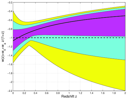
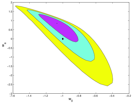
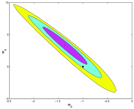
This parametrization can be thought as the parametrization of the DE density instead of $w(z)$. By fitting this model to the observational data, we find that $\chi^{2}=158.07$, $\Omega_{m}=0.29\pm 0.04$, $w_{0}=-1.07^{+0.33}_{-0.28}$ and $w_{a}=0.85^{+0.61}_{-1.38}$. Compared with previous fitting results gong05 , the current data makes a little improvement on the constraint of $w_{a}$. The evolution of $w(z)$ is plotted in Fig. 2 and the contours of $w_{0}$ and $w_{a}$ are shown in Fig. 3. From Fig. 2, we see that at the $3\sigma$ confidence level, $w(z)<0$ for $z<2$, $w(z)$ crosses the $-1$ barrier around $z\sim 0.1$, and the stringent constraint on $w(z)$ happens around $z\sim 0.3$. From the Fisher matrix estimation, we get $z/(1+z)=F_{12}/F_{11}=0.32$, so the sweet spot is around $z=0.47$. This estimation is quite different from what we get, and the main reason is that the distribution of $w_{a}$ is highly non-Gaussian. From Fig. 3, we see that the cosmological constant is more than $1\sigma$ away from the best fit result.

Figure 2: The evolution of $w(z)$ by fitting the model $w(z)=w_{0}+w_{a}z/(1+z)$ to the observational data. The solid line is drawn by using the best fit parameters. The shaded areas show the $1\sigma$, $2\sigma$ and $3\sigma$ errors.

Figure 3: The $1\sigma$, $2\sigma$ and $3\sigma$ contour plots of $w_{0}$ and $w_{a}$ for the model $w(z)=w_{0}+w_{a}z/(1+z)$. The diamond denotes the point corresponding to the cosmological constant.

The second DE parametrization we consider is jbp

$$w(z)=w_{0}+\frac{w_{a}z}{(1+z)^{2}}\ .$$ (12)

The dimensionless DE density is

$$\Omega_{DE}(z)=\Omega_{DE0}(1+z)^{3(1+w_{0})}\exp\left[3w_{a}z^{2}/2(1+z)^{2}\right].$$ (13)

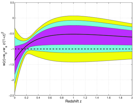
Again this parametrization can also be thought as the parametrization of the DE density. By fitting this model to the observational data, we find that $\chi^{2}=157.11$, $\Omega_{m}=0.28^{+0.04}_{-0.03}$, $w_{0}=-1.37^{+0.58}_{-0.57}$ and $w_{a}=3.39^{+3.51}_{-3.93}$. These constraints are almost at the same level as previous results in gong05 . The evolution of $w(z)$ is plotted in Fig. 4 and the contours of $w_{0}$ and $w_{a}$ are shown in Fig. 5. From Fig. 4, we see that at the $3\sigma$ confidence level, $w(z)<0$ for $z<0.7$, w(z) crosses the $-1$ barrier around $z\sim 0.15$, and the stringent constraint on $w(z)$ happens around $z\sim 0.2$. The sweet spot is estimated to be $z=0.2353$ from the equation $z/(1+z)^{2}=F_{12}/F_{11}=0.1542$. From Fig. 5, we see that the $\Lambda$CDM model is almost $2\sigma$ away from the best fit result.

Figure 4: The evolution of $w(z)$ by fitting the model $w(z)=w_{0}+w_{a}z/(1+z)^{2}$ to the observational data. The solid line is drawn by using the best fit parameters. The shaded areas show the $1\sigma$, $2\sigma$ and $3\sigma$ errors.

Figure 5: The $1\sigma$, $2\sigma$ and $3\sigma$ contour plots of $w_{0}$ and $w_{a}$ for the model $w(z)=w_{0}+w_{a}z/(1+z)^{2}$. The diamond denotes the point corresponding to the cosmological constant.

The last model we consider is alam

$$\Omega_{DE}(z)=A_{1}(1+z)+A_{2}(1+z)^{2}+1-\Omega_{m}-A_{1}-A_{2}.$$ (14)

The EoS parameter $w(z)$ is

$$w(z)=\frac{1+z}{3}\frac{A_{1}+2A_{2}(1+z)}{\Omega_{DE}(z)}-1.$$ (15)

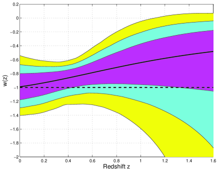
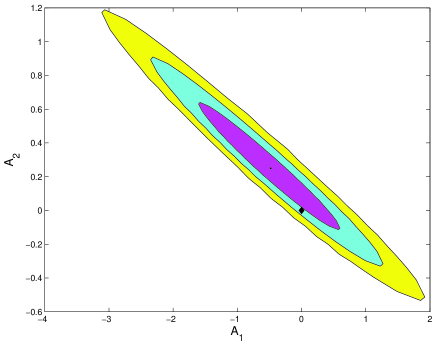
The cosmological constant corresponds to $A_{1}=A_{2}=0$. By fitting this model to the observational data, we find that $\chi^{2}=158.48$, $\Omega_{m}=0.30\pm 0.04$, $A_{1}=-0.48^{+1.36}_{-1.47}$ and $A_{2}=0.25^{+0.52}_{-0.45}$. The evolution of $w(z)$ is plotted in Fig. 6 and the contours of $A_{1}$ and $A_{2}$ are shown in Fig. 7. From Fig. 6, we see that at the $3\sigma$ confidence level, $w(z)<0$ for $z<1.1$ and the stringent constraint on $w(z)$ happens around $z\sim 0.4$. From Fig. 7, we see that the $\Lambda$CDM model is more than $1\sigma$ away from the best fit result. Comparing the value of $\chi^{2}$ of the three models we considered, we find that the second model fits a little bit better than the other two models do.

Figure 6: The evolution of $w(z)$ by fitting the model $\Omega_{DE}(z)=1-\Omega_{m}-A_{1}-A_{2}+A_{1}(1+z)+A_{2}(1+z)^{2}$ to the observational data. The solid line is drawn by using the best fit parameters. The shaded areas show the $1\sigma$, $2\sigma$ and $3\sigma$ errors.

Figure 7: The $1\sigma$, $2\sigma$ and $3\sigma$ contour plots of $A_{1}$ and $A_{2}$. The diamond denotes the point corresponding to the cosmological constant.

IV The geometry of the Universe

In this section, we use the observational data to find out the geometry of our universe. When $k\neq 0$, the luminosity distance becomes

$$d_{\rm L}(z)=\frac{1+z}{H_{0}\sqrt{|\Omega_{k}|}}{\rm sinn}\left[\sqrt{|\Omega_{k}|}\int_{0}^{z}\frac{dz^{\prime}}{E(z^{\prime})}\right],$$ (16)

where ${\rm sinn}(\sqrt{|k|}x)/\sqrt{|k|}=\sin(x)$, $x$, $\sinh(x)$ if $k=1$, 0, $-1$, the parameter $A$ becomes

$$A=\frac{\sqrt{\Omega_{m}}}{0.35}\left[\frac{0.35}{E(0.35)}\frac{1}{|\Omega_{k}|}{\rm sinn}^{2}\left(\sqrt{|\Omega_{k}|}\int_{0}^{0.35}\frac{dz}{E(z)}\right)\right]^{1/3},$$ (17)

and the shift parameter becomes

$$\mathcal{R}=\frac{\sqrt{\Omega_{m}}}{\sqrt{|\Omega_{k}|}}{\rm sinn}\left(\sqrt{|\Omega_{k}|}\int_{0}^{z_{ls}}\frac{dz}{E(z)}\right).$$ (18)

To fit the observational data, we consider the one parameter DE parametrization gong05

$$w(z)=\frac{w_{0}}{1+z}e^{z/(1+z)}.$$ (19)

During both the early and future epoches, $w(z)\rightarrow 0$. The DE density is

$$\Omega_{DE}=\Omega_{DE0}(1+z)^{3}\exp\left(3\omega_{0}e^{z/(1+z)}-3\omega_{0}\right).$$ (20)

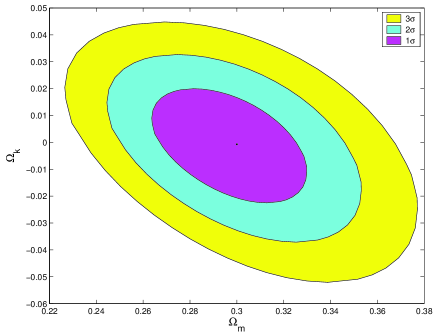
By fitting this model to the observational data, we find that $\chi^{2}=158.85$, $\Omega_{m}=0.30\pm 0.04$, $\Omega_{k}=-0.0007^{+0.032}_{-0.03}$ and $w_{0}=-0.93^{+0.17}_{-0.18}$. The data is also used to fit the $\Lambda$CDM model, the results are $\chi^{2}=160.51$, $\Omega_{m}=0.30\pm 0.03$ and $\Omega_{k}=-0.02\pm 0.02$. This model fits the observational data as well as the $\Lambda$CDM and the two-parameter models do. The contours of $\Omega_{m}$ and $\Omega_{k}$ are shown in Figs. 8 and 9. The errors on $\Omega_{m}$ and $\Omega_{k}$ are almost the same. Comparing with the results in gong05 , we find that the new SN Ia data improves the constraint on $\Omega_{k}$ significantly.

Figure 8: The $1\sigma$, $2\sigma$ and $3\sigma$ contour plots of $\Omega_{m}$ and $\Omega_{k}$ for the parametrization $w(z)=w_{0}\exp[z/(1+z)]/(1+z)$.

Figure 9: The $1\sigma$, $2\sigma$ and $3\sigma$ contour plots of $\Omega_{m}$ and $\Omega_{k}$ for the $\Lambda$CDM model.

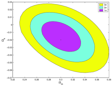
V Discussion

By fitting the simple two-parameter representation of $q(z)$ to the new 182 gold SN Ia data, we find strong evidence of acceleration in the recent past which is consistent with previous studies in sturner ; gong06 . While the evidence of current acceleration is weak from fitting the simple piecewise constant acceleration model to the previous gold SN Ia data sturner and fitting the simple two-parameter representation of $q(z)$ to the 115 nearby Supernova Legacy Survey (SNLS) SN Ia data astier ; gong06 , we find strong evidence of current acceleration by using the gold SN Ia data. The strongest evidence of acceleration again happens around the redshift $z\sim 0.2$. The transition redshift when the Universe underwent the transition from deceleration to acceleration is found to be $z_{t}=0.36^{+0.23}_{-0.08}$ at the $1\sigma$ level.

The new SN Ia data, together with the BAO measurement from SDSS and the shift parameter determined from WMAP3 data, are used to fit three popular DE parameterizations. When we are given the parameterizations $w(z)=w_{0}+w_{a}z/(1+z)$ and $w(z)=w_{0}+w_{a}z/(1+z)^{2}$, the explicit analytical expressions for the DE density can be derived. Alternatively, we can think that we are parameterizing the DE density $\Omega_{DE}(z)$ instead of $w(z)$. The new observational data makes slightly improvement on the constraint of $w_{a}$, while the $\Lambda$CDM model is still consistent with current observational data. Although high redshift SN Ia data provides robust constraint on the property of DE evldh , the stringent constraint on $w(z)$ happens around $z\sim 0.3$. In other words, at the $3\sigma$ confidence level, $w(z)$ is best constrained around the redshift $z\sim 0.3$. Surprisingly, we only have a few SN Ia with redshift around $0.3$ in the current 182 gold SN Ia data. The same result holds for the DE parametrization $\Omega_{DE}(z)=1-\Omega_{m}-A_{1}-A_{2}+A_{1}(1+z)+A_{2}(1+z)^{2}$, although the redshift is now around $z\sim 0.4$. We think this result is quite generic for two-parameter parametrizations. The result also suggests that more SN Ia data with the redshift $z\sim 0.2-0.4$ may be valuable to give strong constraint on $w(z)$. The sweet spot around the redshift $z\sim 0.2-0.4$ may be argued from the Hubble law and the decreasing importance of DE huterer ; weller ; saini : (1) At low redshift, the luminosity distance can be expressed as $H_{0}d_{L}(z)=z+\frac{1}{2}(1-q_{0})z^{2}$. To the linear approximation, it does not depend on the cosmological parameters, so the constraint on the property of DE at low redshift from SN Ia data is not strong; (2) At high redshift, the role of DE diminishes. Depending on the model, the evidence for $w(z)<0$ at high redshift is different.

We also apply the one-parameter parametrization $w(z)=w_{0}\exp(z/(1+z))/(1+z)$ to study the geometry of the Universe. Although the SN Ia data alone does not provide valuable constraint on the geometry, the new combined data improves the constraint on $\Omega_{k}$ significantly. At the $3\sigma$ confidence level, we have $|\Omega_{k}|\lesssim 0.05$ for the model $w(z)=w_{0}\exp(z/(1+z))/(1+z)$ and $-0.064<\Omega_{k}<0.028$ for the $\Lambda$CDM model. It should be stressed that the effect of the heterogeneous nature of the gold SN Ia data on the systematics is also important and it may impose potential problem when combining with WMAP3 data jbp06 ; nesseris05 ; nesseris6b . The more homogeneous SNLS SN Ia data avoids this problem jbp06 ; nesseris05 ; nesseris6b .