On self-sustaining processes in Rayleigh-stable rotating
plane Couette flows and subcritical transition to
turbulence in accretion disks

Abstract

Context. Subcritical transition to turbulence in Keplerian accretion disks is still a controversial issue and some theoretical progress is required in order to determine whether or not this scenario provides a plausible explanation for the origin of angular momentum transport in non-magnetized accretion disks.

Aims. Motivated by the recent discoveries of exact nonlinear steady self-sustaining solutions in linearly stable non-rotating shear flows, we attempt to compute similar solutions in Rayleigh-stable rotating plane Couette flows and to identify transition mechanisms in such flows.

Methods. Numerical simulations (time-stepping approaches) have been employed in most recent studies of the problem. Here, we instead combine nonlinear continuation methods and asymptotic theory to study the nonlinear dynamics of plane Couette flows in Rayleigh-stable regimes.

Results. We obtain exact nonlinear solutions for Rayleigh-stable cyclonic regimes using continuation techniques proposed by Waleffe and Nagata but show that it is not possible to compute solutions for Rayleigh-stable anticyclonic regimes, including Keplerian flow, using similar techniques. We also present asymptotic descriptions of these various problems at large Reynolds numbers that provide some insight into the differences between the non-rotating and Rayleigh-stable anticyclonic regimes and derive some necessary conditions for mechanisms analogous to the non-rotating self-sustaining process to be present in (constant angular momentum) flows on the Rayleigh line.

Conclusions. Our results demonstrate that subcritical transition mechanisms cannot be identified in wall-bounded Rayleigh-stable anticyclonic shear flows by transposing directly the phenomenology of subcritical transition in cyclonic and non-rotating wall-bounded shear flows. Asymptotic developments, however, leave open the possibility that nonlinear self-sustaining solutions may exist in unbounded or periodic flows on the Rayleigh line. These could serve as a starting point to discover solutions in Rayleigh-stable flows, but the nonlinear stability of Keplerian accretion disks remains to be determined.

1 Introduction

Physical mechanisms responsible for turbulent angular momentum transport in Keplerian accretion disks have long been a matter of debate among astrophysicists. While there is convincing evidence that the presence of magnetic fields in disks (Donati et al. 2005) triggers turbulence thanks to a linear magnetorotational instability (MRI, see Velikhov 1959; Chandrasekhar 1960; Balbus & Hawley 1991), purely hydrodynamic sources of turbulence still have to be discovered in some regions of protoplanetary disks which are likely to be decoupled from magnetic fields (Fromang et al. 2002) and in disks forming in binary systems in quiescence, in which MHD turbulence and the associated turbulent transport may die away as a consequence of the smallness of the magnetic Reynolds number (Gammie & Menou 1998).

Studying hydrodynamic transition to turbulence in Keplerian flows is an extremely difficult task for essentially two reasons. On the one hand, there is currently no known local linear instability which could provide a route to turbulence in the non-magnetized Keplerian flow regime. Dubrulle et al. (2005) have pointed out the existence of an instability in stably stratified accretion disks, but its local nature is very unclear (Umurhan 2006; Brandenburg & Dintrans 2006). On the other hand, the linear operators associated with shear flows are mathematically non-normal, which physically means that short-term dynamics (transient algebraic growth) rather than normal modes may play an important role in the process of transition to turbulence (Korycansky 1992; Trefethen et al. 1993; Schmid & Henningson 2000; Chagelishvili et al. 2003; Tevzadze et al. 2003; Yecko 2004; Afshordi et al. 2005; Mukhopadhyay et al. 2005). Several authors (Richard & Zahn 1999; Longaretti 2002) have suggested that subcritical transition may be possible in accretion disks in spite of the stabilizing effect of the Coriolis force, but this point of view has been contested by Balbus et al. (1996), Hawley et al. (1999) and Balbus (2003). The relevance of such mechanisms to the problem of turbulent transport in disks has also been questioned by Lesur & Longaretti (2005), who extrapolated from numerical simulation results that the critical Reynolds number for this kind of process to occur in the Keplerian regime was far too large and the associated angular momentum transport far too small to account for the accretion process. Recently, Balbus & Hawley (2006) have further questioned this transition scenario, basing their argument on the observation that transiently amplified shearing waves are solutions for any amplitude (because their self-interactions are vanishing) and cannot therefore directly trigger turbulence. Balbus & Hawley (2006) and Shen et al. (2006) have also studied the nonlinear evolution of these non-axisymmetric shearing waves using high-resolution simulations and have found that they become unstable to Kelvin-Helmholtz instabilities if they reach a sufficient amplitude. However, the turbulent motions generated this way ultimately die away in the configuration of their simulation.

Most recent theoretical studies of hydrodynamic turbulence in accretion disks have focused on linear transient growth, which is only one part of a full subcritical transition scenario, and is not a sufficient condition for nonlinear instability. Nonlinear dynamics has mostly been studied numerically within the shearing box model (Rogallo 1981) using direct time-stepping approaches. The nonlinear outcome of the transient growth process remains unclear and theoretical progress is required in order to clarify the existence and nature of subcritical transition in Rayleigh-stable (centrifugally stable) rotating shear flows. The aim of this paper is to present some theoretical and numerical arguments that may help to make progress in this direction, and notably to investigate if some nonlinear mechanisms that are crucial for subcritical transition to turbulence in non-rotating shear flows play a role in linearly stable rotating shear flows too. We have been motivated by the vast amount of experimental, numerical and theoretical work that has become available in fluid dynamics in the last ten years and have oriented our study towards one of the most promising avenues of research in that field, namely the self-sustaining process, first identified by Hamilton et al. (1995) for non-rotating plane shear flows. Our hope has been to be able to identify a similar process for Rayleigh-stable rotating shear flows, notably the anticyclonic plane Couette flow on the Rayleigh line, which at first glance presented many similarities with its non-rotating counterpart (Balbus & Hawley 1998). Unlike most recent studies, we have tried to address the fully nonlinear problem using continuation methods, in order to compute accurate nonlinear solutions in different rotation regimes and to pinpoint the physical mechanisms that may give birth to turbulence in these regimes. Our results shed some new light on the nonlinear outcome of linear transient growth on the Rayleigh line and show that it is not possible to identify nonlinear solutions in wall-bounded Rayleigh-stable anticyclonic shear flows using arguments similar to those pertaining to the self-sustaining process in non-rotating shear flows. We also argue that these findings do not rule out the possibility of a subcritical transition scenario in accretion disks, but show that self-sustaining mechanisms in rotating plane shear flows with linearly stable anticyclonic rotation, if they exist, must be qualitatively different from their non-rotating equivalent.

The outline of the paper is as follows. In Sect. 2, we summarize the current understanding of transition to turbulence in shear flows and give a detailed description of the phenomenology of the self-sustaining process for non-rotating shear flows. Section 3 is devoted to the mathematical description of the nonlinear problem that we have been attempting to solve. The numerical tools developed for the purpose of our study are presented in Sect. 4. We then report some numerical results for subcritical transition in cyclonic (Sect. 5) and anticyclonic (Sect. 6) rotating plane Couette flows. Section 7 provides some theoretical insight into the asymptotics of self-sustaining processes at very large Reynolds numbers in order to understand these numerical results and the difficulties in identifying a self-sustaining process so far for linearly stable anticyclonic regimes. A discussion of the results and guidelines for future work are finally presented in Sect. 8.

2 Transition to turbulence in shear flows and the self-sustaining process

To gain some theoretical understanding of the Keplerian problem, it is necessary to come back to the more general problem of hydrodynamic transition to turbulence in shear flows. For a long time, the only classical non-rotating shear flow for which an explanation for transition was available is plane Poiseuille flow with rigid boundaries. The transition was attributed to the linear instability of this flow at a critical Reynolds number $\mathrm{Re}=5572$ (see Orszag (1971); Zahn et al. (1974); Orszag & Patera (1980)), which takes the form of travelling waves. The instability is subcritical and finite amplitude solutions can be tracked down to $\mathrm{Re}=2900$ (Herbert 1976). However, it was noticed that this global critical Reynolds number was rather high compared to the transition value observed experimentally. Studies of secondary instabilities of these travelling waves did not seem to resolve this discrepancy (see e. g. Drissi et al. 1999). Another major problem with this approach was that it applied only to plane Poiseuille flow: plane Couette flow and pipe Poiseuille flow do not have any linear instability and nevertheless become turbulent at moderate values of $\mathrm{Re}$ (the linear stability for all Reynolds numbers of Plane Couette flow with rigid boundaries was demonstrated by Romanov (1973)).

In the last decade, a nonlinear self-sustaining process acting as an organizing center of the dynamics in phase space has been discovered, leading to a new paradigm in the understanding of transition in shear flows. Corresponding exact nonlinear solutions to the Navier-Stokes equations have been identified numerically in plane Poiseuille flow and plane Couette flow with either no-slip or stress-free boundaries (Hamilton et al. 1995; Waleffe 1995, 1997; Schmiegel 1999; Waleffe 2001, 2003), and in pipe Poiseuille flow (Faisst & Eckhardt 2003; Wedin & Kerswell 2004), leading to an elegant solution to the historical problem of transition in pipes (Reynolds 1883). These coherent structures take the form of nonlinear travelling waves or of a steady pattern, depending on the symmetries of the original problem. The critical global transition Reynolds numbers and the mean flow profiles for these solutions prove to be far closer to experimental measurements than predictions made by other theories, and an experimental detection of these structures in pipe Poiseuille flow has been reported recently (Hof et al. 2004). The self-sustaining process as it is understood now is a subtle balance between linear and nonlinear mechanisms. The linear part of the process results physically from the transient growth of a streamwise-independent (axisymmetric in the accretion disk terminology) streamwise velocity field (referred to as the streaks field) which originates from the redistribution of the mean shear by low-amplitude streamwise vortices (or equivalently streamwise rolls). Such a growth is limited to time scales $\mathcal{O}(\mathrm{Re})$ because of the ultimate diffusion of streamwise vortices. This mechanism is called the lift-up effect (Landahl 1980; Butler & Farrell 1992). A steady state can only be achieved thanks to the development of a three-dimensional linear instability of the high-amplitude streaks, which produces a nonlinear feedback that is sufficient to maintain the original rolls field. Note that the linear growth of streamwise-independent structures is a key requirement for the whole process to occur, and that this physical mechanism is a direct consequence of the non-normality of the linear operator. It is also different from and more powerful than the “swing amplification” of streamwise-dependent (non-axisymmetric) Orr-Kelvin shearing waves (Lord Kelvin 1887; Orr 1907; Knobloch 1984; Craik & Criminale 1986; Butler & Farrell 1992). It is worth emphasizing here that the upper and lower branches of these three-dimensional solutions are both unstable to steady and oscillatory modes with the same basic symmetries. As discussed by Waleffe (2001), this does not mean that the original coherent structures are not relevant to transition. On the contrary, they are expected to show up intermittently in the flow, and the fact that they have instabilities ensures that bifurcations to even more complex structures and to turbulence are possible.

Far less is known analytically regarding the stability of spanwise rotating plane shear flows (the spanwise direction is the one perpendicular to the disk plane in an accretion disk). The linear stability properties of such systems depend on the rotation number $R_{\Omega}$, which is proportional to the ratio of the rotation rate $\Omega$ and the background shear rate $S$ (defined here as the negative of the background flow relative vorticity):

$$R_{\Omega}=-\frac{2\Omega}{S}.$$ (1)

This $R_{\Omega}$ is the same as the one defined by Lesur & Longaretti (2005) ($S$ here is $-S$ in their paper but they use $R_{\Omega}=2\Omega/S$) and differs in sign from the definition of Bech & Andersson (1997). Here we assume that $S$ is constant in the shearwise (radial) direction, which corresponds to a plane Couette flow. A necessary condition (known as the Rayleigh criterion) for this flow to become linearly unstable is that $-1<R_{\Omega}<0$, which shows that the flow has to be anticyclonic to be unstable, i. e. that the vorticity of the background flow and the rotation rate have opposite sign. In this so-called Rayleigh-unstable regime, the centrifugal instability is responsible for the transition to turbulence, as observed in both laboratory (Tillmark & Alfredsson 1996; Alfredsson & Tillmark 2005) and numerical (Bech & Andersson 1996, 1997) experiments. This instability is the same as the instability studied by Taylor (1923) in the Taylor-Couette experiment, which exhibits axisymmetric structures called Taylor vortices close to the bifurcation point. On the contrary, rotating plane Couette flow in the cyclonic regime ($R_{\Omega}>0$) and anticyclonic flows with $R_{\Omega}<-1$ are Rayleigh-stable for all $\mathrm{Re}$. Local linearizations of Keplerian flows, which have $R_{\Omega}=-4/3$, are included into this category. From the experimental point of view, turbulence is of course known to be present in plane Couette flow for $R_{\Omega}=0$ (non-rotating plane Couette flow), but it has also been observed for small positive rotation numbers (Tillmark & Alfredsson 1996). Note finally that unlike for non-rotating plane Couette flow, there is no complete proof that rotating plane Couette flow at $R_{\Omega}=-1$ is linearly stable for all Reynolds numbers.

At that point, it should be noted that a strong theoretical connection exists between the nonlinear stability of non-rotating plane Couette flow and the weakly nonlinear behaviour of Rayleigh-unstable Taylor-Couette flow in the narrow gap limit. This link was discovered by Nagata (1988, 1990). He found that the three-dimensional nonlinear self-sustaining steady solutions for non-rotating plane Couette flow (which were unknown at that time and had therefore not been related to any kind of self-sustaining process) could be obtained directly by nonlinear continuation (with respect to the rotation rate) of wavy Taylor vortices, which emerge from a three-dimensional bifurcation of the Taylor vortex flow. For a given range of streamwise wavenumbers, Nagata (1990) showed that these solutions could be continued slightly into the cyclonic regime. Komminaho et al. (1996) performed numerical simulations and discovered that the large-scale structures of turbulence disappeared in the cyclonic regime at $R_{\Omega}=0.06$ for $\mathrm{Re}=750$, in qualitative agreement with the experimental results of Tillmark & Alfredsson (1996).

Whether or not turbulence exists in the Rayleigh-stable, anticyclonic regime (and notably in Keplerian accretion disks) is still very unclear, as mentioned earlier. Richard & Zahn (1999), using data from experiments by Wendt (1933) and Taylor (1936), suggested that transition to turbulence should be observed in a Taylor-Couette flow in that regime at rather modest $\mathcal{O}(10^{5})$ Reynolds numbers, and claimed experimental evidence for this (Richard 2001). Bech & Andersson (1997) found that turbulence disappeared at $R_{\Omega}=-1$ for Reynolds numbers up to $\mathrm{Re}\sim 1300$. Nonlinear stability in the Taylor-Couette problem was also investigated by Garaud & Ogilvie (2005) using a closure model for the Reynolds stresses derived by Ogilvie (2003). They showed that within the framework of this model, nonlinear solutions in the anticyclonic Rayleigh-stable regime should exist if solutions in the cyclonic regime exist, thanks to a symmetry with respect to $R_{\Omega}=-0.5$. Streamwise-independent solutions of the Navier-Stokes equations do have such a symmetry (see also Balbus et al. 1996), but Lesur & Longaretti (2005) pointed out that it is broken when fully three-dimensional solutions of the Taylor-Couette problem are considered, leaving the issue of the existence of nonlinear solutions in the stable anticyclonic regime unsettled. Hawley et al. (1999) and Lesur & Longaretti (2005), using shearing box simulations (Rogallo 1981), observed turbulence for anticyclonic rotation down to $R_{\Omega}=-1.03$ and Lesur & Longaretti (2005), using either shearing box or rigid-boundary simulations, found turbulence at small positive rotation numbers (up to 0.12). The nature of the numerical code (which does not include explicit diffusion) of Hawley et al. (1999) did not allow them to make statements on critical Reynolds numbers for the onset of turbulence in these flows, but the results of Lesur & Longaretti (2005) show good agreement with the experiments of Tillmark & Alfredsson (1996) on the cyclonic side and seem to indicate that transition occurs on the anticyclonic side for $\mathrm{Re}\sim 1500$ at $R_{\Omega}=-1$. Also, their results show that the critical Reynolds number for the appearance of turbulence at more negative rotation numbers increases very rapidly ($\mathrm{Re}_{c}\sim 4\times 10^{4}$ for $R_{\Omega}=-1.03$), which is not consistent with the experimental results of Richard (2001). Ji et al. (2006) have recently performed a new Taylor-Couette experiment. Their results show that quasi-Keplerian flows remain essentially steady at Reynolds numbers up to millions, in agreement with the conclusions of Lesur & Longaretti (2005).

This summary of our current understanding of transition in non-rotating and rotating shear flows makes it clear that we still do not apprehend the whole process in a satisfying way. Some important questions, such as the existence of a some qualitative symmetry with respect to $R_{\Omega}=-0.5$ or the existence of a self-sustaining process in the presence of rotation, remain largely unanswered. From our point of view, these issues have to be addressed theoretically before conclusions on hydrodynamic transition to turbulence in Rayleigh-stable rotating shear flows such as Keplerian flows can be made.

3 Setting up the problem

3.1 Physical model

In order to address this problem, we considered an incompressible spanwise-rotating plane Couette flow between rigid boundaries, which is representative of shear flows that are linearly stable for all Reynolds numbers in the absence of rotation. As is common in the fluid dynamics literature, $(x,y,z)$ stand respectively for the streamwise (azimuthal, $-y$ in the shearing sheet coordinates), shearwise (radial, $x$ in the shearing sheet coordinates) and spanwise (vertical) directions. The shearwise direction is bounded by two rigid walls, so that $-d<y<d$, and $d$ is chosen as unit of length. We further assume that the $x$ and $z$ direction are periodic with spatial periods $L_{x}=2\pi d/\alpha$ and $L_{z}=2\pi d/\beta$ . The background flow reads $\@vec{U}_{B}=Sy\,\@vec{e}_{x}$, the rotation vector is given by $\@vec{\Omega}=\Omega\,\@vec{e}_{z}$ and the constant shear rate $S$ is used to define a time unit. In nondimensional form we therefore have $-1<y<1$ and $\@vec{U}_{B}=y\,\@vec{e}_{x}$. The classical definition of the Reynolds number in plane Couette flow is based on the shear velocity at the boundaries and half of the channel width:

$$\mathrm{Re}=\frac{|S|d^{2}}{\nu},$$ (2)

where $\nu$ is the constant kinematic viscosity of the fluid. The Reynolds number defined above is four times smaller than the ones used by Nagata (1986) and Lesur & Longaretti (2005), and the rotation number, defined in Eq. (1), obeys $R_{\Omega}=-\Omega_{\mbox{\tiny TC}}/\mathrm{Re}_{\mbox{\tiny TC}}$ where the TC index refers to quantities defined in the Taylor-Couette problem by Nagata (1986).

3.2 Equations

The full velocity field, denoted by $\@vec{U}$, is split into $\@vec{U}_{B}$, the original streamwise background flow, and velocity perturbations $\@vec{u}=(u,v,w)$, which include any possible modification of the original background flow. The nondimensional equations governing the evolution of $\@vec{U}$ and of the total pressure $P=P_{B}+p$ (implicitly divided by the constant density $\rho$), where $p$ denotes the pressure perturbation, are the incompressible Navier-Stokes equations, which read

$$\hskip 19.91684pt\frac{\partial\@vec{U}}{\partial t}+\@vec{U}\cdot\@vec{\nabla}\@vec{U}-R_{\Omega}\,\@vec{e}_{z}\times\@vec{U} = -\@vec{\nabla}{P}+\frac{1}{Re}\Delta\@vec{U},$$ (3)

$$\@vec{\nabla}\cdot{\@vec{U}} = 0.$$ (4)

These equations have to be completed by periodic boundary conditions in $x$ and $z$ and by rigid (no-slip) boundary conditions in the $y$ direction (the $x,z$ dependence is omitted here):

$${u(-1)=u(1)=v(-1)=v(1)=w(-1)=w(1)=0,}$$ (5)

Anticipating the numerics, an important point is that these equations reduce to two three-dimensional scalar equations governing the evolution of shearwise velocity $(v)$ and vorticity $(\eta)$ perturbations (Schmid & Henningson 2000):

$$\left(\frac{\partial}{\partial t}-\frac{1}{\mathrm{Re}}\Delta\right)\Delta v+\@vec{P}_{v}\cdot\left(\@vec{U}\cdot\@vec{\nabla}{\@vec{U}}-R_{\Omega}\,\@vec{e}_{z}\times\@vec{U}\right)=0,$$ (6)

$$\left(\frac{\partial}{\partial t}-\frac{1}{\mathrm{Re}}\Delta\right)\eta+\@vec{P}_{\eta}\cdot\left(\@vec{U}\cdot\@vec{\nabla}{\@vec{U}}-R_{\Omega}\,\@vec{e}_{z}\times\@vec{U}\right)=0,$$ (7)

where

$$\hskip 85.35826pt\@vec{P}_{v} = -\@vec{e}_{y}\cdot\@vec{\nabla}\times{\@vec{\nabla}\times{(\cdot)}},$$ (8)

$$\@vec{P}_{\eta} = \@vec{e}_{y}\cdot\@vec{\nabla}\times{(\cdot)},$$ (9)

plus two streamwise and spanwise-independent equations describing the evolution of the mean streamwise and spanwise velocity fields:

$$\left(\frac{\partial}{\partial t}-\frac{1}{\mathrm{Re}}\frac{\partial^{2}}{\partial y^{2}}\right)\left<{u}\right>+\left<{\@vec{e}_{x}\cdot\@vec{U}\cdot\@vec{\nabla}{\@vec{U}}}\right>=0,$$ (10)

$$\left(\frac{\partial}{\partial t}-\frac{1}{\mathrm{Re}}\frac{\partial^{2}}{\partial y^{2}}\right)\left<{w}\right>+\left<{\@vec{e}_{z}\cdot\@vec{U}\cdot\@vec{\nabla}{\@vec{U}}}\right>=0,$$ (11)

where brackets denote $(x,z)$ averages. Note that $\left<v\right>=0$ results from the incompressibility constraint and boundary conditions (5), and that the Coriolis force does not enter Eqs. (10)-(11).

3.3 Symmetries

The fluid motions that will be studied here have several symmetries, which can be used to reduce the computational costs. We will first deal with three-component two-dimensional (streamwise independent) flows (hereinafter 2D-3C), like combined streamwise rolls (vortices) and streaks, which have a reflection symmetry with respect to the $z=0$ plane for a properly chosen phase in $z$. This symmetry reads

$$\mathcal{Z}:(x,y,z)\rightarrow(x,y,-z),\quad(v,\eta)\rightarrow(v,-\eta).$$ (12)

Thanks to the $\mathcal{Z}$ symmetry of the basic 2D-3C flows, fully three-dimensional nonlinear solutions bifurcating from these flows have either the $\mathcal{Z}$ symmetry or the so-called “shift-and-reflect” symmetry given by

$$\mathcal{S}_{2}:(x,y,z)\rightarrow(x+L_{x}/2,y,-z),\quad(v,\eta)\rightarrow(v,-\eta).$$ (13)

A basic 2D-3C solution has both $\mathcal{Z}$ and $\mathcal{S}_{2}$ symmetries but the three-dimensional part of the total velocity field has only one of them. Finally, choosing the $x$-phase of the three-dimensional solution (brackets denote $(x,y)$ averages) such that

$$\Im\left<\eta\exp\,(-i\alpha x)\right>=0\quad\mbox{or}\quad\Im\left<v\exp\,(-i\alpha x)\right>=0,$$ (14)

depending on whether the solution has $\mathcal{S}_{2}$ or $\mathcal{Z}$ symmetry, it is possible to show that for plane Couette flow the velocity field has the following “shift-and-rotate” symmetry:

$$\mathcal{S}_{1}:(x,y,z)\rightarrow(L_{x}/2-x,-y,z+L_{z}/2),\quad(v,\eta)\rightarrow(-v,\eta).$$ (15)

The forementioned symmetries have been named according to the nomenclature used in Wedin & Kerswell (2004) with $(x,y,z)$ here corresponding to $(z,r,\phi)$ in their paper on pipe Poiseuille flow (not to be confused with the cylindrical coordinates sometimes used for accretion disks).

3.4 Comments on the model

Before we start describing our results, let us briefly comment on our choices regarding this physical model. We will discuss two points: incompressibility and boundary conditions. Accretion disks are fully compressible and our assumption of incompressibility may appear as a limitation. We fully support the idea that sound waves may play an important role in the nonlinear dynamics of accretion disks, notably by destabilizing coherent vortical structures (Broadbent & Moore 1979; Bodo et al. 2005) and by limiting their extent because of the need to maintain causal acoustic contact, and that compressible physics should be included in any accretion disk study aiming at being realistic. However, the fact that disks are compressible does not mean that incompressible dynamics is unimportant in this environment. Our motivation in this study has been to identify such fundamental incompressible processes, which are major actors of the transition to turbulence in non-rotating shear flows. The self-sustaining process described in Sect. 2 does not require any compressible effect and is already fairly complex, so our choice represents a natural simplification to tackle the corresponding rotating problem.

The second point has to do with our choice of a wall-bounded flow model, which may not be relevant to the physics of accretion disks, notably because walls are responsible for the appearance of boundary layers and global modes. There are two reasons for this choice here: first, investigating exact nonlinear dynamics using continuation methods usually requires that solutions be steady in a given frame of reference, and finite shearing boxes do not admit steady non-axisymmetric ($x$-dependent) solutions (non-axisymmetry is mandatory to have sustained hydrodynamic turbulent angular momentum transport in Rayleigh-stable and Rayleigh-neutral flows). In fact, using our set of coordinates and dimensional units, the shearing-periodic boundary condition on $\@vec{u}(x,y,z,t)$ is

$$\@vec{u}(x,y+L_{y},z,t)=\@vec{u}(x-SL_{y}t,y,z,t).$$ (16)

If $\@vec{u}(x,y,z,t)$ depends on $x$ (its first argument) but not on $t$ (its fourth argument) then Eq. (16) cannot be satisfied because the r.h.s. depends on time, while the l.h.s. does not. For this reason, the finite shearing box does not offer a practical framework to investigate the exact nonlinear dynamics of shear flows. It may admit non-axisymmetric solutions that are periodic in time, but it seems technically difficult to obtain them using standard numerical methods. The second reason has to do with the phenomenology of rotating shear flow turbulence in laboratory. At first glance, the fact that only wall-bounded flows admit steady three-dimensional nonlinear solutions may be problematic for self-sustaining process theories in accretion disks. However, we note that the phenomenology of the onset of turbulence looks very similar in unbounded and wall-bounded flows: for instance, transition Reynolds numbers observed for cyclonic rotation in shearing boxes or in configurations with rigid boundaries are comparable (Lesur & Longaretti 2005). Also, experiments on wall-bounded Rayleigh-stable anticyclonic plane shear flows face exactly the same difficulty as shearing box simulations, i. e. turbulence dies away for $R_{\Omega}$ close to -1 (Tillmark & Alfredsson 1996; Bech & Andersson 1997) at Reynolds numbers $\mathcal{O}(10^{3})$ for both types of set-ups. Studying the analytically and numerically simpler case of wall-bounded flows may thus prove useful to understand the unbounded problem too.

4 Numerical methods

Bearing in mind the symmetry of Couette flow with respect to the centre of the channel, we aimed at computing steady nonlinear solutions of the previous set of equations (in plane Poiseuille flow, which does not have this symmetry, solutions would be travelling). For this purpose, we developed two codes: a full nonlinear continuation code similar to those of Waleffe (2003) and Wedin & Kerswell (2004) to compute exact three-dimensional nonlinear steady solutions of Eqs. (5)-(6)-(7)-(10)-(11) thanks to a Newton iteration algorithm, and a two-dimensional linear stability code to find accurate initial guesses for the nonlinear code. In both codes, discretization is done on a Gauss-Lobatto grid (Chebyshev collocation) in the shearwise direction and a Fourier spectral representation is used in the $x$ and $z$ directions. Boundary conditions are implemented using differentiation matrices computed with the DMSuite package (Weidemann & Reddy 2000). In the continuation code, nonlinear terms are computed in physical space and the steady nonlinear equations are solved in spectral-physical-spectral space using a direct LAPACK solver to perform Newton iterations. The stability code makes uses of either the direct LAPACK eigenvalue solver, which computes the whole spectrum of eigenvalues of the discretized operator, or the iterative Arnoldi ARPACK solver to compute individual eigenmodes. The nonlinear code was first checked with a two-dimensional subcritical test problem, namely the Orr-Sommerfeld problem for a no-slip plane Poiseuille flow (Zahn et al. 1974; Herbert 1976) and the full three-dimensional version was successfully tested by reproducing the bifurcation diagram for no-slip non-rotating plane Couette flow obtained by Waleffe (2003) for $(\alpha,\beta)=(0.577,1.15)$ (see below). Dealiasing was implemented but did not prove necessary to obtain accurate solutions in most cases. The linear solver was tested by calculating the limits and critical wavenumbers for the centrifugal instability and by quantitatively reproducing results obtained for the inflectional instability of streaks (Waleffe 1995, 1997; Reddy et al. 1998) in both plane Couette flow and plane Poiseuille flow, for which the instability of streaks takes the form of a travelling wave (non-zero eigenfrequency). Pseudo-arclength continuation was implemented to follow branches of solutions. The previously mentioned symmetries can be turned on or off in the nonlinear code in order to reach higher resolutions. We checked that the introduction of the symmetries module of the code gave the same results as the full problem for mild resolutions. We would finally like to emphasize here that the numerical methods used in our calculations for spatial differentiation have spectral (exponential) convergence, and that the maximum affordable resolutions $(N_{x},N_{y},N_{z})=(32,24,32)$ used in this paper (which require approximately one Gigabyte of memory) allow for the computation of fairly complex velocity fields with an excellent precision.

5 Cyclonic rotation

5.1 Computation of exact nonlinear solutions in non-rotating plane Couette flow

In this section, we report results obtained for cyclonic rotation. In order to reach this regime, we first computed steady non-rotating plane Couette flow solutions using the same technique as Waleffe (2003) (see also Wedin & Kerswell (2004) for a similar approach for the pipe Poiseuille flow problem). The maximum resolution used for these calculations was $(N_{x},N_{y},N_{z})=(32,24,32)$, which is similar to the resolution of Waleffe (2003), and the $\mathcal{S}_{1}$ and $\mathcal{S}_{2}$ symmetries were used in the code to compute fully three-dimensional solutions.

The basic idea of this forcing approach, as we will call it in the remainder of the paper, is to compute fully three-dimensional nonlinear solutions of the forced Navier-Stokes equations using Newton iteration, then decreasing progressively the forcing term until a solution for zero forcing is found. In practice, an initial guess is required to perform this calculation. In this study, we chose $(\alpha,\beta)=(0.577,1.15)$, for which the global critical Reynolds number for the self-sustaining process is known to be minimized, and set $\mathrm{Re}=150$. The determination of the initial guess was done in two steps. The first step was to compute the 2D-3C streamwise-independent part of the flow, denoted by $(u_{\mbox{\scriptsize 2D}},v_{\mbox{\scriptsize 2D}},w_{\mbox{\scriptsize 2D}})$ and the second step was to compute the three-dimensional instability of this 2D-3C flow. We first focus on the first step, which relies on the physics of the lift-up effect in order to calculate a combined rolls and streaks velocity field. The simplest streamwise rolls structure is given by the most slowly decaying solution of the linear Stokes problem for the streamwise vorticity $\omega=\exp\,(\lambda t/\mathrm{Re})\,\omega_{s}(y,z)$

$$\lambda\,\omega_{s}=\Delta\,\omega_{s},$$ (17)

where $\lambda$ is negative. For rigid no-slip boundary conditions and a $z$-periodicity of the rolls $\beta=1.15$, the least stable eigenvalue is given by $\lambda=-9.27306$. The corresponding Stokes velocity field is

$$(v_{s},w_{s})=(-\partial_{z}\Delta^{-1}\omega_{s},\partial_{y}\Delta^{-1}\omega_{s}).$$ (18)

The physics of the lift-up effect is such that $\mathcal{O}(1/\mathrm{Re})$ streamwise rolls generate $\mathcal{O}(1)$ streamwise velocity, so we chose the amplitude of the rolls to be

$$(v_{\mbox{\scriptsize 2D}},w_{\mbox{\scriptsize 2D}})=\frac{A}{\mathrm{Re}}\frac{(v_{s},w_{s})}{\mbox{max}(v_{s})},$$ (19)

where $A$ is assumed to be $\mathcal{O}(1)$. As shown by the sign of $\lambda$, this rolls field decays viscously, so that the following $\mathcal{O}(1/\mathrm{Re}^{2})$ forcing term $\@vec{F}$

$$(F_{x},F_{y},F_{z})=\frac{|\lambda|}{\mathrm{Re}}(0,v_{\mbox{\scriptsize 2D}},w_{\mbox{\scriptsize 2D}})=\frac{A|\lambda|}{\mathrm{Re}^{2}}\frac{(v_{s},w_{s})}{\mbox{max}(v_{s})}$$ (20)

had to be included in the Navier-Stokes equations in order to compensate for viscous diffusion. The determination of the 2D-3C part of the initial guess was finally completed by solving the linear problem

$$\left(\frac{1}{\mathrm{Re}}\Delta-v_{\mbox{\scriptsize 2D}}\frac{\partial}{\partial y}-w_{\mbox{\scriptsize 2D}}\frac{\partial}{\partial z}\right)u_{\mbox{\scriptsize 2D}}=v_{\mbox{\scriptsize 2D}}\frac{\partial U_{B}}{\partial y}$$ (21)

for the $\mathcal{O}(1)$ streaks field $u_{\mbox{\scriptsize 2D}}$. For a well-chosen $z$ phase, this 2D-3C field has $\mathcal{Z}$ and $\mathcal{S}_{2}$ symmetries.

The three-dimensional part of the initial guess was then determined by computing a neutral instability mode of the rolls and streaks field for the chosen value of $\alpha$ using the linear stability solver. For $\alpha=0.577$, this mode, which has $\mathcal{S}_{2}$ symmetry, is marginally stable when the forcing amplitude is $A\simeq 4.4$. Using the total rolls and streaks field and a small three-dimensional neutral mode perturbation as an initial guess, we finally succeeded in computing an exact three-dimensional nonlinear steady forced solution using the Newton solver. In order to obtain a solution for zero forcing, we then only had to reduce the amplitude of the forcing term step-by-step down to zero amplitude and to follow the corresponding forced solution using the nonlinear continuation code. The bifurcation diagram with respect to the forcing amplitude $A$ is shown in Fig. 1. In this plot, the $y$-averaged amplitude of the $k_{x}=\alpha$ mode of the shearwise vorticity $\eta$

$$\mbox{Amp}_{\mbox{\scriptsize 3D}}=\Re\int_{-1}^{1}\!\!\!\left<\eta\exp\,(-i\alpha x)\right>\mbox{d}y$$ (22)

is used to measure the amount of three-dimensionality of the solution. As shown in this diagram, the whole procedure works because the bifurcation to three-dimensional solutions is subcritical with respect to the forcing amplitude. Note also that $A$ is effectively $\mathcal{O}(1)$ at the bifurcation point.

Figure 1: Bifurcation diagram of forced nonlinear solutions in non-rotating plane Couette flow with $(\alpha,\beta)=(0.577,1.15)$ with respect to the forcing amplitude $A$, for $\mathrm{Re}=150$. $\mbox{Amp}_{\mbox{\scriptsize 3D}}$, defined by Eq. (22), is used to measure the amount of three-dimensionality in the full nonlinear solution. The resolution $(N_{x},N_{y},N_{z})=(32,24,32)$ was used to perform this calculation.

Before cyclonic continuation was attempted, the non-rotating plane Couette flow solution obtained previously was finally continued with respect to the Reynolds number in order to obtain the full bifurcation diagram for the chosen aspect ratio. The Reynolds number of the saddle-node bifurcation point is $\mathrm{Re}=127.7$ (see Fig. 2).

Figure 2: Bifurcation diagram for non-rotating plane Couette flow with $(\alpha,\beta)=(0.577,1.15)$ with respect to $\mathrm{Re}$. The nondimensional wall shear rate $|\partial\left<{U}\right>/\partial y|(y=\pm 1)$ is used as a measure of nonlinearity (for the laminar flow, $|\partial\left<{U}\right>/\partial y|(\pm 1)=1$).

5.2 Continuation in the cyclonic regime

The bifurcation diagram obtained in the previous paragraph was then used to compute solutions in the $R_{\Omega}>0$ region by performing continuation with respect to $R_{\Omega}$. Solutions for several Reynolds numbers were continued from the lower branch of Fig. 2. A turning point is found systematically at a critical rotation number depending on the chosen Reynolds number. The solution then evolves back to zero rotation number and reaches the upper branch of the non-rotating plane Couette flow bifurcation diagram. For the forementioned maximum affordable resolution, solutions could be obtained for Reynolds numbers up to 500. Note that we suffered from a lack of numerical resolution for $\mathrm{Re}=500$. The continuation curve is incomplete in that case and is given for illustrative purposes only, because the corresponding results are probably not very accurate. Unfortunately, it is not possible to increase the resolution of this experiment further by a significant amount because of both memory and CPU requirements. For instance, the LAPACK linear solver has algorithmic complexity $\mathcal{O}(N^{3})$, where $N$ is the system size, so that doubling the resolution in even only one direction would be prohibitive (computing one point of the continuation curves using the present resolution already takes several hours on a 3 GHz processor). Branches of solutions obtained at various Reynolds numbers are plotted in Fig. 3 and a snapshot of isovorticity surfaces and streamlines for the solution at the turning point at $\mathrm{Re}=303$ and $R_{\Omega}=0.017$ is shown in Fig. 4. Anticipating a comparison with results for anticyclonic rotation, we also present in Fig. 5 a bifurcation diagram for $\mathrm{Re}=303$ similar to the one obtained by Nagata (1990), showing both the 2D-3C Taylor vortices branch in the linearly unstable weakly anticyclonic regime and its connection with the three-dimensional wavy Taylor vortices penetrating into the cyclonic region.

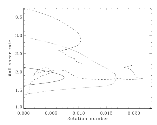
Figure 3: Branches of three-dimensional nonlinear solutions obtained in the cyclonic region for $\mathrm{Re}=150$ (full line), $\mathrm{Re}=303$ (dotted line) and $\mathrm{Re}=500$ (dashed line). A turning point corresponding to a critical rotation number is found for any $\mathrm{Re}$. The $\mathrm{Re}=500$ calculation suffered from a lack of numerical resolution.

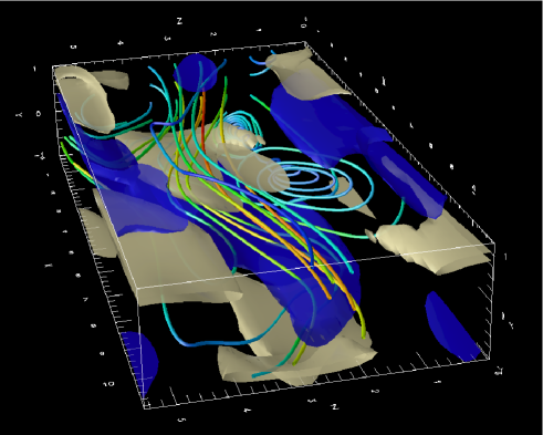
Figure 4: Positive (light brown) and negative (dark blue) isovorticity surfaces and randomly selected streamlines for the nonlinear solution located at $\mathrm{Re}=303$ and $R_{\Omega}=0.017$.

Figure 5: Bifurcation diagram for Taylor vortices (full line) showing their connection with three-dimensional rotating self-sustaining solutions (dotted line) at $\mathrm{Re}=303$. The dash-triple dotted curve shows the centrifugal stability limit. $(\alpha,\beta)=(0.577,1.15)$.

It is interesting to compare the critical $R_{\Omega}-\mathrm{Re}$ curve obtained from our computations with already published experimental and numerical work. Figure 6 shows that the critical $\mathrm{Re}$ obtained for the exact coherent structures is smaller than the critical $\mathrm{Re}$ for the onset of turbulence in cyclonic experiments for $\mathrm{Re}=150$ and $\mathrm{Re}=303$ (note again that the $\mathrm{Re}=500$ point in that plot is purely illustrative due to the lack of numerical resolution). The critical $\mathrm{Re}$ is seen to increase with increasing cyclonic rotation, similarly to experiments. A possible interpretation for these observations is that the values obtained in our study for $(\alpha,\beta)$ parameters that minimize the global critical Reynolds number for the non-rotating plane Couette flow provide lower bounds on the transition $\mathrm{Re}$ in the cyclonic regime as well. Since Tillmark & Alfredsson (1996) and Lesur & Longaretti (2005) used a different aspect ratio in their experiments, larger Reynolds numbers may be required in their set-up to obtain turbulence. An alternative explanation is that the exact coherent structures computed here do not allow for a precise determination of the turbulence threshold in a real experiment and only give a rough estimate for the critical $\mathrm{Re}$, because the actual transition process involves not only these solutions but all their possible instabilities, as mentioned previously.

Figure 6: Critical Reynolds number for exact three-dimensional nonlinear solutions for $(\alpha,\beta)=(0.557,1.15)$ as a function of the rotation number $R_{\Omega}$ (+), compared to the experimental data obtained by Tillmark & Alfredsson (1996) ($\diamond$) for the onset of turbulence and the numerical data by Komminaho et al. (1996) ($\triangle$). The $\mathrm{Re}=500$ point only gives a qualitative indication of the actual critical value because of the lack of resolution for the corresponding numerical experiment. The numerical results of Lesur & Longaretti (2005) for shearing box simulations match those obtained by Tillmark & Alfredsson (1996) and are not reproduced here.

6 Anticyclonic rotation

Several arguments regarding the existence of turbulence in Keplerian flows have been based on a possible symmetry with respect to $R_{\Omega}=-0.5$. In this section, we report some continuation experiments in the anticyclonic region, which notably show that the self-sustaining process present in non-rotating or weaky cyclonic shear flows ($R_{\Omega}\simeq 0$) cannot be transposed into the $R_{\Omega}\simeq-1$ regimes and that more complex nonlinear structures have to be searched for to find subcritical transition (if any) in this region.

6.1 Finding a starting point for continuation

Nonlinear continuation methods require a starting point, which is usually a bifurcation point. This bifurcation can have a physical origin, when a linear instability like the centrifugal instability is present. In that case, continuation is straightforward. When there are no linear instabilities, a possibility is to include an extra artificial term in the original equations to trigger a linear instability that would otherwise be absent, and to study the subsequent nonlinear dynamics when this artificial term is gradually removed. This is how Nagata (1990) proceeded in order to find three-dimensional solutions of non-rotating plane Couette flow. By adding a small amount of anticyclonic rotation to the original Couette flow, he caused the background flow to become centrifugally unstable and followed the 2D-3C Taylor vortices (axisymmetric structures with small amplitude streamwise rolls and strong streamwise velocity) into the nonlinear domain. In this regime, Taylor vortices become unstable to three-dimensional wavy Taylor vortices at a critical Reynolds number depending on the amount of rotation of the system. The interesting finding of Nagata (1990) was that he was able to follow this three-dimensional solution down to zero rotation, thanks to a proper nonlinear feedback of the three-dimensional structures on the streamwise rolls originally generated by the centrifugal instability. In the previous section, we proceeded in a similar way to find non-rotating solutions, but instead of adding a small amount of anticyclonic rotation originally, we used the same method as Waleffe (2003) to sustain the rolls field, by adding an artificial forcing term in the streamwise vorticity equation. A third possibility, found by Clever & Busse (1992), is to cause the Couette flow to become unstable to convection by imposing a supercritical temperature gradient in the shearwise direction in order to force the rolls field, and then perform a nonlinear continuation of the secondary instabilities of the convection rolls when the temperature gradient is suppressed. In spite of their a priori rather different characteristics, all these approaches lead to the same result. The reason for this is linear transient growth via the lift-up effect. All these methods sustain weak streamwise rolls which give rise to a finite amplitude streaks velocity field, as a consequence of the spanwise redistribution of streamwise velocity. The instability of streaks, whatever the origin of streamwise rolls is, results from the presence of inflection points in the spanwise streak profile (Jones 1981).

In order to investigate the nonlinear dynamics in the rotating Keplerian regime, a proper starting point is required too, and a major problem is to find it. Unfortunately, we did not find a nonlinear connection between the non-rotating plane Couette flow solutions and the strongly anticyclonic region. As shown in Fig. 5, the three-dimensional lower branch of solutions that crosses the $R_{\Omega}=0$ line joins the two-dimensional Taylor vortex branch at some very small negative $R_{\Omega}$, and we had difficulties in following the three-dimensional upper branch for $R_{\Omega}<-0.5$ for the parameters of Fig. 5 (the solutions on this branch turn into nonlinear travelling waves (non-zero phase speed) at $R_{\Omega}\simeq-0.216$, similarly to what has been observed in experiments (Andereck et al. 1986; Nagata 1990)). Thus, another starting point must be found in order to study the region of large negative $R_{\Omega}$. It seemed difficult to start directly from the Keplerian regime, which is very far from any linear instability point, so our idea was to start from more convenient rotating regimes and to try to continue possible solutions towards $R_{\Omega}=-4/3$. We experimented with two ideas for $R_{\Omega}=-1$ or close to minus one.

The first working hypothesis, inspired by Nagata (1990), was to start from values of $R_{\Omega}$ larger than but close to -1 in order to trigger a centrifugal instability, and to study the nonlinear behaviour of secondary instabilities of the Taylor vortices in that regime, when $R_{\Omega}$ is made closer to -1 (centrifugal instability approach). The second technique, similar to that used in Sect. 5 to obtain solutions for $R_{\Omega}=0$, was motivated by a very strong analogy and near-symmetry regarding linear theory between the $R_{\Omega}=0$ and $R_{\Omega}=-1$ regimes. From the strictly linear point of view, Antkowiak & Brancher (2006) have shown that the lift-up effect, which occurs for $R_{\Omega}=0$, has an equivalent for $R_{\Omega}=-1$, christened the “anti lift-up” effect. This equivalence can be seen by considering the linear equations describing the evolution of the streamwise velocity field $u$ and of the streamwise vorticity $\omega$ (the rolls field) in plane Couette flow with system rotation:

$$\frac{\partial u}{\partial t} = -(R_{\Omega}+1)v+\frac{1}{\mathrm{Re}}\Delta u,$$ (23)

$$\hskip 56.9055pt\frac{\partial\omega}{\partial t} = -R_{\Omega}\frac{\partial u}{\partial z}+\frac{1}{\mathrm{Re}}\Delta\,\omega.$$ (24)

For $R_{\Omega}=0$, a streamwise velocity field is generated by redistribution of shear by the streamwise rolls velocity field, leading to strong transient amplification and the formation of streaks. There is no source term in Eq. (24) and any streamwise vorticity perturbation must decay viscously in this linear framework. For $R_{\Omega}=-1$, strong streamwise vorticity can be generated transiently by the Coriolis force acting on the streamwise velocity. The streamwise velocity equation (23) has no source term in that case because the Coriolis force acting on the rolls exactly compensates the redistribution of the mean shear by the rolls, so that streamwise velocity perturbations decay viscously. Transient growth observed for $R_{\Omega}=-1$ can also be interpreted as an epicyclic oscillation of infinite period, since the epicyclic frequency is zero in this regime (Antkowiak & Brancher 2006). Pushing the analogy with the non-rotating case further and now considering nonlinear effects, the generation of finite-amplitude rolls by the anti lift-up effect may then allow for the development of three-dimensional instabilities that could behave in a similar way to their $R_{\Omega}=0$ counterparts and feedback on a weak streamwise velocity field, thus leading to a self-sustaining process for $R_{\Omega}=-1$. The procedure in that case is to set directly $R_{\Omega}=-1$, to artificially force a weak streaks field in order to amplify streamwise rolls, and to follow the nonlinear development of the instabilities of the rolls when removing progressively the forcing term (forcing approach).

6.2 Centrifugal instability approach

We start by describing results obtained in the first working hypothesis. Using both linear stability codes and nonlinear continuation, we identified streamwise-independent Taylor vortices bifurcating from the spanwise-rotating background Couette flow at various $R_{\Omega}$ larger than but very close to -1. In practice, the bifurcation to Taylor vortices occurs when the Taylor number

$$\mathrm{Ta}=-16\mathrm{Re}^{2}R_{\Omega}(1+R_{\Omega})$$ (25)

exceeds 1707, so that the critical $R_{\Omega}$ depends only slightly on $\mathrm{Re}$ at large $\mathrm{Re}$. We chose $\beta=1.5585$, which is the critical wavenumber for this instability (in the Taylor-Couette experiment, this would be $\beta=3.117$ because $2d$ is used as unit of length in that case). The structure of the full velocity field of the Taylor vortices in this rotating regime is quite different from the one at small $R_{\Omega}$: close to $R_{\Omega}=-1$, the streaks field has a lower amplitude than for small $R_{\Omega}$, which is a consequence of the absence of the lift-up effect. The secondary instabilities of the Taylor vortices close to the Rayleigh line $R_{\Omega}=-1$ are therefore different from those at small $R_{\Omega}$, whose inflectional nature is due to the shape and amplitude of the streamwise velocity field in that regime. This marks a fundamental difference between the two regimes and already hints that the argument on symmetries of solutions with respect to $R_{\Omega}=-0.5$ is limited. Due to the $\mathcal{Z}$ symmetry of the Taylor vortices, two steady three-dimensional instabilities can be found, with either $\mathcal{S}_{2}$ (wavy Taylor vortices, hereinafter WTV) or $\mathcal{Z}$ (twisted Taylor vortices, hereinafter TTV) symmetry. These instabilities have been identified by Nagata (1986) and TTVs have been observed experimentally by Andereck et al. (1983) for $R_{\Omega}\sim-0.8$. Finally, some steady subharmonic instabilities with spanwise wavelength twice the wavelength of the Taylor vortices and an instability with non-zero phase speed are also present (see Nagata 1988). These latter instabilities are poor candidates for continuation into the Rayleigh-stable regime because they have been reported experimentally for $-0.5>R_{\Omega}>-0.8$ only (see Andereck et al. 1983). Consequently, they have not been considered in this study.

Close to the Rayleigh line, the first unstable three-dimensional mode (when $\mathrm{Re}$ is increased) is the wavy Taylor vortex mode for the numerically accessible range of $\mathrm{Re}$ (see Fig. 7 for a comparison between the growth rate of WTVs and TTVs for some of the parameters used here). In Fig. 8, we show the corresponding bifurcation diagrams in the vicinity of $R_{\Omega}=-1$ for $\mathrm{Re}=500$ and $\mathrm{Re}=1500$. The bifurcations to 2D-3C Taylor vortices are supercritical with respect to $R_{\Omega}$ and the associated branches of nonlinear solutions do not cross the Rayleigh line $R_{\Omega}=-1$. Independently of $\mathrm{Re}$, the secondary bifurcations to three-dimensional WTVs are unfortunately also supercritical and the corresponding branches of solutions do not approach the centrifugal stability limits either, unlike their counterpart at $R_{\Omega}\sim 0$, in spite of having the same $\mathcal{S}_{2}$ symmetry (compare with Fig. 5). The same remarks apply to TTVs. This demonstrates clearly that the phenomenology of self-sustaining processes at $R_{\Omega}=0$ cannot be transposed directly into the $R_{\Omega}=-1$ regime, even though analogous linear transient amplification mechanisms exist in each of these regimes.

Figure 7: Growth rate of the three-dimensional instability modes of the Taylor vortices as a function of the streamwise wavenumber $\alpha$ for $R_{\Omega}=-0.97875$, $\mathrm{Re}=500$ and $\beta=1.5585$. Full line: wavy vortex mode. Dotted line: twisted vortex mode. Nonlinear continuation from the bifurcation point is initialized by adding a small amount of neutral modes with $\alpha=1$ to the Taylor vortex flow.

Figure 8: Bifurcation diagrams in the $R_{\Omega}\sim-1$ region for $(\alpha,\beta)=(1,1.5585)$ and Reynolds numbers $\mathrm{Re}=500$ (lower full, dotted and dashed lines) and $\mathrm{Re}=1500$ (upper full, dotted and dashed lines). The resolution is $(N_{y},N_{z})=(24,48)$ for the Taylor vortex branches (full lines) and $(N_{x},N_{y},N_{z})=(16,24,48)$ for the WTV branches (dotted lines) and TTV branches (dashed lines). The dashed-triple dotted line is the Rayleigh line. Continuation was stopped at smaller values of $R_{\Omega}$ for $\mathrm{Re}=1500$ due to insufficient numerical resolution.

6.3 Pitfalls of the forcing approach

As mentioned earlier, using a forcing approach similar to that presented in Sect. 5 appeared as a plausible alternative to the centrifugal instability approach in order to identify a self-sustaining process at $R_{\Omega}=-1$. Such an attempt was further encouraged by the work of Wedin & Kerswell (2004), who managed to identify a self-sustaining process in non-rotating pipe Poiseuille flow by continuing forced nonlinear solutions, whereas Barnes & Kerswell (2000) had previously been unable to continue nonlinear solutions obtained for a rotating pipe Poiseuille flow down to zero rotation.

The simplest (and possibly naive) way of tackling the problem was to include an artificial forcing term

$$F_{x}(y,z)=\frac{A}{\mathrm{Re}^{2}}\left(\beta^{2}+\frac{\pi^{2}}{4}\right)\cos\beta z\cos\left(\frac{\pi y}{2}\right)$$ (26)

in the streamwise velocity equation in the Rayleigh-neutral $R_{\Omega}=-1$ regime in order to sustain the following streamwise velocity field against viscous dissipation:

$$u(y,z)=\frac{A}{\mathrm{Re}}\cos\beta z\cos\left(\frac{\pi y}{2}\right).$$ (27)

The forcing amplitude $A$ is assumed to be $\mathcal{O}(1)$, as in the non-rotating problem (see Waleffe 1995, 2003), in order to generate possibly unstable finite-amplitude $\mathcal{O}(1)$ streamwise thanks to the Coriolis force acting on the $\mathcal{O}(1/\mathrm{Re})$ streamwise velocity field. Note that unlike for $R_{\Omega}=0$, there is no need to solve numerically a Stokes problem for the streamwise velocity here, because the boundary conditions on $u$ make it possible to use exact expressions like Eq. (26) for the forcing term.

Initializing the Newton solver with the streamwise velocity field (27) and streamwise forcing term (26) plus a streamwise rolls field with streamwise vorticity $\omega$ being the solution of the linear problem

$$\Delta\,\omega=-\mathrm{Re}\frac{\partial u}{\partial z},$$ (28)

nonlinear steady 2D-3C forced solutions could be obtained for various forcing amplitudes (see Fig. 9). However, their properties turned out to be quite different from the prediction of linear theory that the streamwise rolls velocity field be $\mathcal{O}(\mathrm{Re})$ larger than the streamwise velocity field. One of the reasons for this difference is that the rolls feed back on the streamwise velocity field which generates them via the anti lift-up effect and sweep it close to the boundaries. In comparison, the corresponding effect at $R_{\Omega}=0$ would be the advection of axisymmetric structures like rolls by the streaks field (the $u\,\partial_{x}$ operator), which is strictly zero due to the streamwise-independence of the rolls and streaks pattern. Therefore, the analogy between $R_{\Omega}=0$ and $R_{\Omega}=-1$ breaks down when nonlinearity is included, at least for the forcing term used here (the precise reasons for this break down and the choice of a suitable forcing term will be further discussed in Sect. 7). The problem becomes even more apparent when computing the stability of these 2D-3C solutions to three-dimensional infinitesimal perturbations with wavenumber $\alpha$. For $\mathrm{Re}=500$ and $(\alpha,\beta)=(0.8,1.5585)$ for instance, bifurcation to three-dimensional solutions with $\mathcal{Z}$ symmetry occurs for $A=\mathcal{O}(10^{3})$ only, whereas bifurcation occurs for $A=\mathcal{O}(1)$ in the $R_{\Omega}=0$ case. Furthermore, the first three-dimensional instability found for $R_{\Omega}=-1$ is supercritical with respect to the forcing amplitude (Fig. 9) and subsequent three-dimensional nonlinear solutions cannot be tracked down to zero forcing (compare with Fig. 1 for $R_{\Omega}=0$).

This second numerical attempt confirms the conclusions drawn from the centrifugal instability approach, namely that a self-sustaining process close to the Rayleigh line, if any, must act quite differently from its non-rotating counterpart. It could be argued that our values of $\mathrm{Re}$ are too small to observe anything interesting in the anticyclonic regime, or that the chosen aspect ratio does not allow for three-dimensional self-sustained solutions. We performed the same kind of computations with different aspect ratios for Reynolds numbers up to approximately 1500 but did not notice any qualitative change in the bifurcation diagrams, which always show bifurcation to three-dimensional solutions at large $A$ and supercritical behaviour with respect to the forcing amplitude.

Figure 9: Bifurcation diagram with respect to the forcing amplitude $A$ for $R_{\Omega}=-1$, $(\alpha,\beta)=(0.8,1.5585)$ and $\mathrm{Re}=500$. The full line curve is the branch of 2D-3C forced solutions and the dotted line curve is the three-dimensional branch of solutions with $\mathcal{Z}$ symmetry. The bifurcation to these three-dimensional solutions occurs for $A=834.7$ and is supercritical with respect to the forcing amplitude.

7 Asymptotic description of self-sustaining processes

The numerical results presented in the previous section illustrate the difficulty of identifying self-sustaining processes in Rayleigh-stable regimes. However, there is currently no mathematical proof that such solutions do not exist, so that it worth attempting to understand why they cannot be found in plane Couette flow on the Rayleigh line and under which circumstances they could be found. In this section, we provide some analytical arguments based on an asymptotic description of the problem at large $\mathrm{Re}$ which, together with the numerical results, highlight the fundamental differences between the $R_{\Omega}=0$ and $R_{\Omega}=-1$ regimes in plane Couette flow. Starting with the non-rotating case, we obtain a two-dimensional formulation for the solutions of the lower branch of the non-rotating self-sustaining process at very large $\mathrm{Re}$. We then consider several possible asymptotic descriptions of three-dimensional solutions close to the Rayleigh line and demonstrate why the actual Taylor vortices generated in this regime in plane Couette flow cannot lead to a rotating self-sustaining process, unlike their $-R_{\Omega}\ll 1$ counterparts. We finally show that self-sustaining solutions on the Rayleigh-line may only exist if the 2D-3C part of the flow satisfies nontrivial solvability conditions.

7.1 Non-rotating Couette flow

7.1.1 Basic equations

Following Sect. 3, perturbations $\@vec{u}=(u,v,w)$ and $p$ to the non-rotating plane Couette flow $\@vec{U}_{B}=y\,\@vec{e}_{x}$ satisfy the nonlinear equation

$$(\partial_{t}+y\partial_{x}+\@vec{u}\cdot\@vec{\nabla})\,\@vec{u}+v\,\@vec{e}_{x}=-\@vec{\nabla}p+\epsilon\Delta\@vec{u},$$ (29)

together with suitable boundary conditions and the constraint

$$\@vec{\nabla}\cdot\@vec{u}=0.$$ (30)

The parameter $\epsilon=1/\mathrm{Re}$ will be used in the following to perform an asymptotic expansion.

7.1.2 Streamwise averaging

Let an overbar denote averaging in the streamwise ($x$) direction, for which periodic boundary conditions apply. Then $\@vec{u}$ and $p$ can be separated into “mean” and “wave” parts, i. e.

$$\@vec{u}(x,y,z,t)=\bar{}\@vec{u}(y,z,t)+\@vec{u}^{\prime}(x,y,z,t),$$ (31)

$$p(x,y,z,t)=\bar{p}(y,z,t)+p^{\prime}(x,y,z,t),$$ (32)

with $\overline{\@vec{u}^{\prime}}={\bf 0}$ and $\overline{p^{\prime}}=0$. We also separate $\bar{}\@vec{u}$ into toroidal (streamwise) and poloidal (shearwise and spanwise) parts, parallel and perpendicular to the averaging direction:

$$\bar{}\@vec{u}=\bar{u}\,\@vec{e}_{x}+\bar{}\@vec{u}_{\mathrm{p}}.$$ (33)

The mean (toroidal and poloidal) and wave parts of Eq. (29) are then

$$(\partial_{t}+\bar{}\@vec{u}_{\mathrm{p}}\cdot\@vec{\nabla})\,\bar{u}+\bar{v}=\epsilon\Delta\bar{u}+F_{x},$$ (34)

$$(\partial_{t}+\bar{}\@vec{u}_{\mathrm{p}}\cdot\@vec{\nabla})\,\bar{}\@vec{u}_{\mathrm{p}}=-\@vec{\nabla}\bar{p}+\epsilon\Delta\bar{}\@vec{u}_{\mathrm{p}}+\@vec{F}_{\mathrm{p}},$$ (35)

$$(\partial_{t}+y\partial_{x}+\bar{}\@vec{u}\cdot\@vec{\nabla})\,\@vec{u}^{\prime}+\@vec{u}^{\prime}\cdot\@vec{\nabla}\bar{}\@vec{u}+\@vec{u}^{\prime}\cdot\@vec{\nabla}\@vec{u}^{\prime}+\@vec{F}+v^{\prime}\,\@vec{e}_{x}=-\@vec{\nabla}p^{\prime}+\epsilon\Delta\@vec{u}^{\prime},$$ (36)

with

$$\@vec{\nabla}\cdot\bar{}\@vec{u}_{\mathrm{p}}=\@vec{\nabla}\cdot\@vec{u}^{\prime}=0,$$ (37)

where

$$\@vec{F}=-\overline{\@vec{u}^{\prime}\cdot\@vec{\nabla}\@vec{u}^{\prime}}$$ (38)

is the mean force associated with the wave. We also define

$$\@vec{G}=\@vec{\nabla}\times\@vec{F}.$$ (39)

Since $\bar{}\@vec{u}_{\mathrm{p}}$ is a solenoidal two-dimensional velocity field we can write it in terms of a streamfunction $\psi(y,z,t)$:

$$\bar{}\@vec{u}_{\mathrm{p}}=\@vec{\nabla}\times(\psi\,\@vec{e}_{x}).$$ (40)

The associated streamwise vorticity is

$$\omega=-\Delta\psi.$$ (41)

We therefore replace equations (34) and (35), taking the curl of the latter to eliminate $\bar{p}$, with

$$\partial_{t}\bar{u}-\frac{\partial(\psi,\bar{u})}{\partial(y,z)}+\bar{v}=\epsilon\Delta\bar{u}+F_{x},$$ (42)

$$\partial_{t}\omega-\frac{\partial(\psi,\omega)}{\partial(y,z)}=\epsilon\Delta\omega+G_{x}.$$ (43)

The reason that streamwise-independent solutions cannot be self-sustaining is that the streamwise vorticity $\omega$ satisfies an advection–diffusion equation with no source term (since $\@vec{G}$ originates from the streamwise-dependent wave parts of the solution). For a self-sustaining solution, the mean and wave parts must interact cooperatively.

7.1.3 Asymptotic reduction

Remembering that the streamwise velocity field is strongly amplified by the lift-up effect and is consequently far larger than the poloidal velocity field, we seek steady asymptotic solutions in the limit of very large Reynolds numbers ($\epsilon\ll 1$), of the form

$$\bar{}\@vec{u}=\bar{u}_{0}(y,z)\,\@vec{e}_{x}+\epsilon\bar{}\@vec{u}_{1}(y,z)+\cdots,$$ (44)

$$\@vec{u}^{\prime}=\epsilon\@vec{u}_{1}^{\prime}(x,y,z)+\cdots,$$ (45)

$$p^{\prime}=\epsilon p_{1}^{\prime}(x,y,z)+\cdots.$$ (46)

At first order, these are required to satisfy

$$-\frac{\partial(\psi_{1},\bar{u}_{0})}{\partial(y,z)}+\partial_{z}\psi_{1}=\Delta\bar{u}_{0},$$ (47)

$$(y+\bar{u}_{0})\partial_{x}\@vec{u}_{1}^{\prime}+(\@vec{u}_{1}^{\prime}\cdot\@vec{\nabla}\bar{u}_{0}+v_{1}^{\prime})\,\@vec{e}_{x}=-\@vec{\nabla}p_{1}^{\prime}.$$ (48)

At second order, we have

$$-\frac{\partial(\psi_{1},\omega_{1})}{\partial(y,z)}=\Delta\omega_{1}+G_{x2},$$ (49)

with

$$\omega_{1}=-\Delta\psi_{1},$$ (50)

$$\@vec{\nabla}\cdot\@vec{u}_{1}^{\prime}=0,$$ (51)

$$\@vec{G}_{2}=-\@vec{\nabla}\times\overline{\@vec{u}_{1}^{\prime}\cdot\@vec{\nabla}\@vec{u}_{1}^{\prime}}.$$ (52)

These equations are closed. Equation (48) for the wave is linear and can be solved by Fourier analysis in $x$. All the equations are therefore reduced to a two-dimensional form. This approach leads to a simplified set of equations which are just a reduced version of the full problem of determining exact self-sustaining solutions. Since the wave involves a single Fourier harmonic, in some sense we have achieved a radical spectral truncation of the three-dimensional problem, yet this is fully supported by the asymptotic analysis. The two main advantages of this set of equations are that (i) the equations are two-dimensional; (ii) there are no small parameters and therefore no small scales to resolve, since the Reynolds number has been scaled out. The amplitude of the wave is arbitrary since it satisfies a homogeneous linear equation. For a domain of fixed size, the amplitude of the wave needs to be chosen so that $\bar{u}_{0}$ has the right amplitude to give rise to a marginally stable wave. Alternatively, the amplitude of the wave can be left as a free parameter and the streamwise wavenumber (or periodicity length) adjusted to allow the marginally stable wave to exist.

The agreement between this analysis and the self-sustaining process in non-rotating plane Couette flow is demonstrated in Fig. 10 and Fig. 11. Figure 10 shows the evolution with respect to $\mathrm{Re}$ of the ratio between the vertical ($z$) kinetic energy contained in the $(k_{x},k_{z})=(\alpha,\beta),(2\alpha,\beta),(3\alpha,\beta)$ Fourier modes and in the $(k_{x},k_{z})=(\alpha,\beta)$ mode at $y=0.707$, for the non-rotating self-sustaining solutions of the lower branch of Fig. 2. At larger $\mathrm{Re}$, the energy contained in the $k_{x}>\alpha$ modes becomes negligible compared to the energy contained in the fundamental $k_{x}=\alpha$ mode, which confirms the prediction made in the previous paragraph that the problem can be solved using only one Fourier harmonic asymptotically. Figure 11 shows that the expansion (44) is very well satisfied by the non-rotating solutions of the lower branch. The streamwise velocity amplitude remains approximately constant and $\mathcal{O}(1)$ for increasing $\mathrm{Re}$, while the poloidal velocity amplitude decreases like $1/\mathrm{Re}$, as expected for a first order quantity in $\epsilon$.

Figure 10: Vertical ($z$) kinetic energy ratio between either $(k_{x},k_{z})=(\alpha,\beta)$ (full line), $(k_{x},k_{z})=(2\alpha,\beta)$ (dotted line) or $(k_{x},k_{z})=(3\alpha,\beta)$ (dashed line) modes and the $(k_{x},k_{z})=(\alpha,\beta)$ mode ($y=0.707$) for the lower branch of non-rotating self-sustaining solutions, as a function of $\mathrm{Re}$. The bump obtained for $\mathrm{Re}>500$ and $k_{x}=3\alpha$ can be explained by the fact that an error tolerance of $10^{-6}$ for the energy was allowed in these computations and that the $(N_{y},N_{z})=(24,32)$ resolution starts to be insufficient for such values of $\mathrm{Re}$.

Figure 11: Maximum of streamwise velocity perturbations $u$ (full line) and of poloidal velocity perturbations $\sqrt{v^{2}+w^{2}}$ (dotted line) for the lower branch of non-rotating self-sustaining solutions, as a function of $\mathrm{Re}$. The dashed line corresponds to a function proportional to $1/\mathrm{Re}$.

One strategy for solving the reduced system would be similar to Waleffe’s approach to the full problem. One can initially set the wave amplitude to zero and replace the forcing term $G_{x2}$ by an artificial force of suitable form, then solve the coupled equations for the “roll” $\psi_{1}$ and “streak” $\bar{u}_{0}$ resulting from this forcing and adjust the wavenumber $\alpha$ to locate a marginally stable wave. If the “feedback” $G_{x2}$ has the same sign and a roughly similar spatial form to the artificial forcing, then the solution can be continued by adding a small amount of wave and reducing the artificial forcing down to zero. If $\alpha$ is fixed in this process, the amplitude of the wave will be adjusted in a self-consistent way. However, we have not carried out such a procedure.

7.2 Asymptotics on the Rayleigh line

As demonstrated in Fig. 10 and Fig. 11, the asymptotics for $R_{\Omega}=0$ are very successful in describing how the actual the self-sustaining process operates in non-rotating plane Couette flow. Recalling that the non-rotating solutions are connected to secondary instabilities of Taylor vortices for small unstable rotation (Fig. 5), it is clear that the asymptotic expansion (44) is satisfied for $-R_{\Omega}\ll 1$ as well with the Coriolis force playing the role of $\@vec{F}$, provided that $-R_{\Omega}\sim\epsilon^{2}$ (or equivalently that the Taylor number defined in Eq. (25) is fixed). This shows that considering the slightly unstable rotating regime allows to capture the essential properties of the non-rotating self-sustaining process.

Here, we similarly analyse the properties of the actual Taylor vortex flow close to the Rayleigh line and its relations with solutions at $R_{\Omega}=-1$, and demonstrate why continuation to $R_{\Omega}<-1$ regimes through three-dimensional solutions is not possible in the same way as in the $R_{\Omega}\sim 0$ region in plane Couette flow. Introducing a critical amount of rotation $R_{\Omega}=-1$ to study self-sustaining behaviour on the Rayleigh line, our equations become

$$(\partial_{t}+y\partial_{x}+\@vec{u}\cdot\@vec{\nabla})\,\@vec{u}+u\,\@vec{e}_{y}=-\@vec{\nabla}p+\epsilon\Delta\@vec{u},$$ (53)

$$\@vec{\nabla}\cdot\@vec{u}=0$$ (54)

(note the $u\,\@vec{e}_{y}$ term here instead of the $v\,\@vec{e}_{x}$ term in Eq. (29)). Then

$$(\partial_{t}+\bar{}\@vec{u}_{\mathrm{p}}\cdot\@vec{\nabla})\,\bar{u}=\epsilon\Delta\bar{u}+F_{x},$$ (55)

$$(\partial_{t}+\bar{}\@vec{u}_{\mathrm{p}}\cdot\@vec{\nabla})\,\bar{}\@vec{u}_{\mathrm{p}}+\bar{u}\,\@vec{e}_{y}=-\@vec{\nabla}\bar{p}+\epsilon\Delta\bar{}\@vec{u}_{\mathrm{p}}+\@vec{F}_{\mathrm{p}},$$ (56)

$$(\partial_{t}+y\partial_{x}+\bar{}\@vec{u}\cdot\@vec{\nabla})\,\@vec{u}^{\prime}+\@vec{u}^{\prime}\cdot\@vec{\nabla}\bar{}\@vec{u}+\@vec{u}^{\prime}\cdot\@vec{\nabla}\@vec{u}^{\prime}-\overline{\@vec{u}^{\prime}\cdot\@vec{\nabla}\@vec{u}^{\prime}}+u^{\prime}\,\@vec{e}_{y}=\!-\@vec{\nabla}p^{\prime}+\epsilon\Delta\@vec{u}^{\prime}$$ (57)

with

$$\@vec{\nabla}\cdot\bar{}\@vec{u}_{\mathrm{p}}=\@vec{\nabla}\cdot\@vec{u}^{\prime}=0.$$ (58)

Writing $\bar{}\@vec{u}_{\mathrm{p}}=\@vec{\nabla}\times(\psi\,\@vec{e}_{x})$ and $\omega=-\Delta\psi$, this time we have

$$\partial_{t}\bar{u}-\frac{\partial(\psi,\bar{u})}{\partial(y,z)}=\epsilon\Delta\bar{u}+F_{x},$$ (59)

$$\partial_{t}\omega-\frac{\partial(\psi,\omega)}{\partial(y,z)}-\partial_{z}\bar{u}=\epsilon\Delta\omega+G_{x}.$$ (60)

The reason that streamwise-independent solutions cannot be self-sustaining is now that the streamwise velocity satisfies an advection–diffusion equation with no source term. Recalling that we are looking for a self-sustaining process in the $R_{\Omega}=-1$ regime, this time we would like to take advantage of the linear anti lift-up effect present in this regime to perform the asymptotic expansion. The anti lift-up effect predicts generation of streamwise rolls $\mathcal{O}(1/\epsilon)$ larger than the streamwise velocity field, which led us to consider two possibilities for asymptotic expansions.

7.2.1 $\mathcal{O}(\epsilon)$ streamwise rolls

A natural asymptotic expansion on the Rayleigh line is obtained by considering the symmetry of 2D-3C Taylor vortices with respect to $R_{\Omega}=-0.5$. If $(u,v,w)$ describes a Taylor vortex solution at $R_{\Omega}$, it can be shown that $(-R_{\Omega}/(R_{\Omega}+1)\,u,v,w)$ is a Taylor vortex solution at $R_{\Omega}^{\prime}=-(R_{\Omega}+1)$. For a given Taylor number, $-R_{\Omega}(R_{\Omega}+1)\sim\epsilon^{2}$, which means that if $u$ is the streamwise velocity component of a Taylor vortex at $-R_{\Omega}\ll 1$, then the streamwise velocity component of the corresponding Taylor vortex at $R_{\Omega}^{\prime}=-(R_{\Omega}+1)$ close to -1 is proportional to $\epsilon^{2}u$. For slightly supercritical Taylor numbers and $-R_{\Omega}\ll 1$, $v$ and $w$ are $\mathcal{O}(\epsilon)$ and $u$ is $\mathcal{O}(1)$. In the symmetry transformation, the rolls field remains $\mathcal{O}(\epsilon)$, while the $u$ field becomes $\mathcal{O}(\epsilon^{2})$ close to $R_{\Omega}=-1$. Put differently, for slightly supercritical Taylor numbers, the streamwise velocity for $-R_{\Omega}\ll 1$ is $\mathcal{O}(1/\epsilon)$ larger than the poloidal velocity, which is consistent with the lift-up effect present in the limit $R_{\Omega}=0$, while for $R_{\Omega}$ slightly larger than -1, the poloidal velocity field is $\mathcal{O}(1/\epsilon)$ larger than the streamwise velocity, which is consistent with the anti lift-up effect present in the limit $R_{\Omega}=-1$. Applying this symmetry transformation to the $R_{\Omega}=0$ asymptotic expansion (44), we obtain the following expansion at $R_{\Omega}=-1$:

$$\bar{}\@vec{u}=\epsilon\bar{}\@vec{u}_{\mathrm{p}1}(y,z)+\epsilon^{2}\bar{}\@vec{u}_{2}(y,z)+\cdots.$$ (61)

Since the amplitude of this 2D-3C flow is small compared to the amplitude of the background flow, no secondary instabilities can be expected. In fact, any marginal three-dimensional secondary solution $(\@vec{u}^{\prime},p^{\prime})$ must obey

$$y\,\partial_{x}\@vec{u}^{\prime}+u^{\prime}\@vec{e}_{y}=-\@vec{\nabla}{p^{\prime}}$$ (62)

at leading order in that case. The rolls field is not involved in this inviscid linear equation, whose only known solutions are simply 2D-3C marginal Taylor vortices on the Rayleigh line that are not compatible with the requirement that $\overline{\@vec{u}^{\prime}}=\@vec{0}$.

The previous analysis therefore highlights one of the major differences between small $R_{\Omega}$ and $R_{\Omega}\simeq-1$ in rotating plane Couette flow: for $-R_{\Omega}\ll 1$, secondary instabilities of the Taylor vortex flow occur for Taylor numbers close to the critical Taylor number for the onset of the centrifugal instability because the Taylor vortex flow is already dominated by $\mathcal{O}(1)$ streaks in the slightly supercritical regime. For instance, the bifurcation to three-dimensional solutions in Fig. 5 occurs for a Taylor number which is less than two times supercritical. For $R_{\Omega}\simeq-1$ and similar weakly supercritical Taylor numbers, there is no such secondary instability because the Taylor vortex velocity field is only $\mathcal{O}(\epsilon)$ in that case. The secondary instabilities computed in Sect. 6 only appear at highly supercritical Taylor numbers. For instance, the Taylor number for which a secondary instability occurs for $\mathrm{Re}=500$ in Fig. 8 is $\sim 200$ times supercritical. The nature of these instabilities remains unclear. They may be related to the presence of strong velocity gradients in thin shear layers and boundary layers that form at large Taylor numbers, when nonlinearities (notably advection of the streamwise velocity by the rolls) become important (see Fig. 12). Similar conclusions can be drawn when using the forcing term defined in Eq. (26) instead of the centrifugal approach, because the structure of the corresponding 2D-3C forced solutions looks very much like the structure of the nonlinear Taylor vortices for $R_{\Omega}$ close to -1.

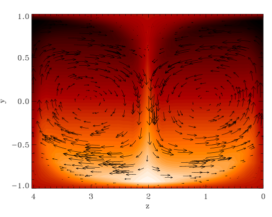
Figure 12: Streamwise velocity $u$ (color scale) and poloidal $(v,w)$ velocity perturbations (arrows) of the nonlinear Taylor vortex flow for $\beta=1.5585$, $R_{\Omega}=-0.995$ and $\mathrm{Re}=5000$, corresponding to $\mathrm{Ta}=1166\,\mathrm{Ta}_{\mathrm{c}}$.

7.2.2 $\mathcal{O}(1)$ streamwise rolls ?

As shown previously, an essential requirement for non-rotating self-sustaining process and three-dimensional dynamics for $-R_{\Omega}\ll 1$ is that secondary instabilities of $\mathcal{O}(1)$ structures are present. In the light of these remarks, we finally attempt to derive an asymptotic expansion for $R_{\Omega}=-1$ taking advantage of the anti lift-up effect, that would allow for bifurcations of an $\mathcal{O}(1)$ $x$-independent velocity field. We seek steady solutions of the form (see Ogilvie & Lubow (2006) for a similar expansion in a different context):

$$\bar{}\@vec{u}=\bar{}\@vec{u}_{\mathrm{p}0}(y,z)+\epsilon\bar{}\@vec{u}_{1}(y,z)+\epsilon^{2}\bar{}\@vec{u}_{2}(y,z)+\cdots,$$ (63)

$$\@vec{u}^{\prime}=\epsilon\@vec{u}_{1}^{\prime}(x,y,z)+\cdots,$$ (64)

$$p^{\prime}=\epsilon p_{1}^{\prime}(x,y,z)+\cdots.$$ (65)

From zeroth to second order, these are required to satisfy

$$-\frac{\partial(\psi_{0},\omega_{0})}{\partial(y,z)}=0,$$ (66)

$$-\frac{\partial(\psi_{0},\bar{u}_{1})}{\partial(y,z)}=0,$$ (67)

$$-\frac{\partial(\psi_{0},\omega_{1})}{\partial(y,z)}-\frac{\partial(\psi_{1},\omega_{0})}{\partial(y,z)}-\partial_{z}\bar{u}_{1}=\Delta\omega_{0},$$ (68)

$$(y\partial_{x}+\bar{}\@vec{u}_{\mathrm{p}0}\cdot\@vec{\nabla})\,\@vec{u}_{1}^{\prime}+\@vec{u}_{1}^{\prime}\cdot\@vec{\nabla}\bar{}\@vec{u}_{\mathrm{p}0}+u_{1}^{\prime}\,\@vec{e}_{y}=-\@vec{\nabla}p_{1}^{\prime},$$ (69)

$$-\frac{\partial(\psi_{0},\bar{u}_{2})}{\partial(y,z)}-\frac{\partial(\psi_{1},\bar{u}_{1})}{\partial(y,z)}=\Delta\bar{u}_{1}+F_{x2},$$ (70)

with

$$\omega_{0}=-\Delta\psi_{0},$$ (71)

$$\omega_{1}=-\Delta\psi_{1},$$ (72)

$$\@vec{\nabla}\cdot\@vec{u}_{1}^{\prime}=0,$$ (73)

$$\@vec{F}_{2}=-\overline{\@vec{u}_{1}^{\prime}\cdot\@vec{\nabla}\@vec{u}_{1}^{\prime}}.$$ (74)

Note that a zeroth-order equation must be satisfied here because of the presence of nonlinear self-interaction terms in the streamwise vorticity equation, contrary to the $R_{\Omega}=0$ case where the zeroth-order terms were strictly vanishing thanks to the streamwise-indepence of the zeroth-order streaks. There is also no equivalent to Eq. (67) in the non-rotating problem. The meaning of these two zeroth-order and first-order equations is that advection by the rolls, although it does not affect the overall energy budget, dominates over viscous and Coriolis terms.

We now drop the subscript on $\psi_{0}$ and introduce a right-handed non-orthogonal coordinate system $(x,\tau,\psi)$ based on the leading-order streamlines, where $\tau$ is the travel time measured along a streamline from its intersection with some reference curve. The Jacobian determinant for this transformation is $\partial(y,z)/\partial(\tau,\psi)=1$. The preceding equations then become

$$\partial_{\tau}\omega_{0}=0,$$ (75)

$$\partial_{\tau}\bar{u}_{1}=0,$$ (76)

$$\partial_{\tau}\omega_{1}-(\partial_{\tau}\psi_{1})\partial_{\psi}\omega_{0}-\partial_{z}\bar{u}_{1}=\partial_{\tau}(g^{\tau\psi}\partial_{\psi}\omega_{0})+\partial_{\psi}(g^{\psi\psi}\partial_{\psi}\omega_{0}),$$ (77)

$$\partial_{\tau}\bar{u}_{2}-(\partial_{\tau}\psi_{1})\partial_{\psi}\bar{u}_{1}=\partial_{\tau}(g^{\tau\psi}\partial_{\psi}\bar{u}_{1})+\partial_{\psi}(g^{\psi\psi}\partial_{\psi}\bar{u}_{1})+F_{x2},$$ (78)

where $g^{ij}$ are the inverse metric coefficients. The unknown quantities $\omega_{1}$ and $\bar{u}_{2}$ are eliminated by integrating with respect to $\tau$. Defining the circulation on the streamline labelled by $\psi$ to be

$$\Gamma(\psi)=\int g^{\psi\psi}\,\mathrm{d}\tau,$$ (79)

where the integral is along the full length of the streamline, the following solvability conditions now need to be satisfied:

$$\frac{\mathrm{d}}{\mathrm{d}\psi}\left(\Gamma\frac{\mathrm{d}\omega_{0}}{\mathrm{d}\psi}\right)+\int(\partial_{z}\bar{u}_{1})\,\mathrm{d}\tau=0,$$ (80)

$$\frac{\mathrm{d}}{\mathrm{d}\psi}\left(\Gamma\frac{\mathrm{d}\bar{u}_{1}}{\mathrm{d}\psi}\right)+\int F_{x2}\,\mathrm{d}\tau=0.$$ (81)

They state that the diffusion of the $x$-independent streamwise vorticity must be balanced by the Coriolis force acting on the streamwise mean velocity $\bar{u}_{1}$, while the diffusion of the $x$-independent streamwise velocity must be balanced by a wave flux (or by a streamwise force in the absence of three-dimensional motions). Finally, the first order equations for the “wave” read

$$(y\partial_{x}+\bar{}\@vec{u}_{\mathrm{p}0}\cdot\@vec{\nabla})\,\@vec{u}_{1}^{\prime}+\@vec{u}_{1}^{\prime}\cdot\@vec{\nabla}\bar{}\@vec{u}_{\mathrm{p}0}+u_{1}^{\prime}\,\@vec{e}_{y}=-\@vec{\nabla}p_{1}^{\prime},$$ (82)

$$\@vec{\nabla}\cdot\@vec{u}_{1}^{\prime}=0.$$ (83)

These equations are linear and can in principle be solved by Fourier analysis in $x$, as in the $R_{\Omega}=0$ case.

To summarize, the asymptotic scenario at $R_{\Omega}=-1$ can be realized if i) a particular distribution of streamwise vorticity satisfying Eq. (66) can be generated thanks to an artificial forcing term satisfying the solvability conditions (80)-(81) ii) the three-dimensional instabilities of this forced flow have the ability to replace the force thanks to their nonlinear feedback on the streamwise-independent part of the flow. In order to satisfy the first requirement, it may notably prove necessary to break the point reflection symmetry

$$(y,z)\rightarrow(-y,L_{z}/2-z),\quad(u,v,w,\omega)\rightarrow(-u,-v,-w,\omega),$$ (84)

of Taylor vortices which causes the streamwise “forcing” term averaged over closed streamlines in Eq. (81) to vanish. In the light of the developments presented in this section, relaxing the constraint of the presence of rigid boundaries that are responsible for the formation of boundary layers may also help to make progress. The fact that transition for $R_{\Omega}\leq 1$ has only been observed in shearing boxes so far seems to support this view. However, we have been unable to isolate such a flow in the course of our investigations. As mentioned in Sect. 3, standard continuation methods are not appropriate to compute solutions in shearing boxes and only theory or direct time-stepping calculations such as those performed by Hawley et al. (1999), Lesur & Longaretti (2005) or Shen et al. (2006) may be able to provide some further insight in that case. An alternative possibility would be to consider a remapping of the shearwise coordinate to obtain an unbounded shear flow between $-\infty<y<+\infty$ and to use nonlinear continuation techniques for such a flow.

8 Discussion and conclusions

In this paper, we have tried to build on the current understanding of transition in non-rotating shear flows in order to isolate exact nonlinear solutions of the Navier-Stokes equations in Rayleigh-stable rotating shear flows and to identify a possible route to turbulence in such flows, including Keplerian flows. On the one hand, we have shown that nonlinear mechanisms act differently on the Rayleigh line, even though analogous transient linear growth processes exist in both types of flows. We have notably computed exact nonlinear solutions for no rotation and for cyclonic rotation but have not succeeded in isolating solutions for $R_{\Omega}=-1$ and smaller using similar techniques. Using the asymptotic approach presented in Sect. 7, we have shed some light on the differences between the two regimes and have demonstrated quantitatively that one cannot transpose straightforwardly the nonlinear stability properties of non-rotating shear flows and the phenomenology of non-rotating self-sustaining processes into the $R_{\Omega}=-1$ regime. In particular, our results show that transition in the narrow gap Taylor-Couette experiment beyond the Rayleigh line, if any, cannot occur through a self-sustaining mechanism analogous to the one pertaining to non-rotating plane Couette flow. On the other hand, our findings do not rule out subcritical transition in Rayleigh-stable shear flows. Finding a way to satisfy the requirements of Eqs. (66)-(80)-(81) may help to discover self-sustaining solutions on the Rayleigh line, which would then offer an interesting starting point for a possible continuation towards $R_{\Omega}=-4/3$. We have argued in Sect. 7 that the presence of walls may prevent such solutions in plane Couette flow with $R_{\Omega}=-1$ and that solutions with the right self-sustaining asymptotic properties may only be found in unbounded or periodic domains.

An alternative to a streamwise rolls-based scenario is that the transition relies on the existence of shearwise rolls, as suggested by Lesur & Longaretti (2005). However, such structures are likely to be transient due to the ambient shear, and it seems difficult to identify a steady self-sustaining process involving them using continuation. This possibility leads us to finally come back to the Keplerian problem and to discuss the recent results of Balbus & Hawley (2006) and Shen et al. (2006) regarding the nonlinear outcome of the transient amplification of non-axisymmetric shearing waves in this regime. Balbus & Hawley (2006) have notably questioned transition to turbulence via this process by showing that shearing waves (even three-dimensional ones) do not have any self-interactions and are therefore exact nonlinear solutions of the equations. We would like to emphasize that nonlinear interactions of transiently amplified structures are not a necessary condition for subcritical transition. Bypass transition in shear flows was highlighted by Trefethen et al. (1993), who argued that this mechanism could trigger turbulence if initial perturbations could reach finite amplitude and interact nonlinearly. But a very simple model for the nonlinear interactions was used at that time, and Waleffe (1995) showed (an argument similar to the one by Balbus & Hawley (2006)), using the full Navier-Stokes equations, that the finite-amplitude streaks generated by the lift-up effect did not feedback on the streamwise rolls directly, leaving the outcome of transient growth and the existence of self-sustaining solutions very uncertain. The real breakthrough of Waleffe (1995), however, was to notice that these spanwise modulated structures became unstable to three-dimensional disturbances when they reached finite amplitudes, which allowed him to discover the full self-sustaining process of which this instability is a crucial piece. In fact, both Balbus & Hawley (2006) and Shen et al. (2006) have found that the transient amplification of shearing waves leads to fairly complex dynamical behaviour as well, even though the nonlinear self-interactions of these structures are vanishing, because such waves become unstable to Kelvin-Helmholtz instabilities when they reach finite amplitude. These authors did not observe subsequent self-sustaining behaviour for the range of parameters explored in their simulations, but more investigations on this problem may be needed before definite negative conclusions can be made. To be complete, it should also be mentioned that the presence of a nonlinear saturation mechanism for transiently amplified structures is not a sufficient condition for subcritical transition either: one of the reasons why a simple self-sustaining process based on the anti lift-up effect cannot occur for wall-bounded shear flows in the $R_{\Omega}=-1$ regime is precisely the nonlinear advection of the streamwise velocity field by linearly amplified streamwise rolls. Finally, we emphasize that following the nonlinear evolution of shearing waves does not ensure that the whole nonlinear dynamical behaviour in Rayleigh-stable regimes has been explored. For instance, the nonlinear cyclonic solutions reported here do not come out of the transient amplification of non-axisymmetric shearing waves. Instead, they are connected to non-rotating solutions which owe their existence to the transient growth of axisymmetric structures. Even though we have not been able to isolate nonlinear coherent structures in the anticyclonic Rayleigh-neutral regime in this study, solutions in the Keplerian regime, if they exist, may well have a connection with nonlinear solutions at $R_{\Omega}=-1$, for which linear axisymmetric transient growth should be present through the anti lift-up effect. The numerical results of Lesur & Longaretti (2005) seem to indicate that transition at $R_{\Omega}=-1$ is possible (at least in shearing boxes) and that a connection with Rayleigh-stable regimes exists, at least for a limited interval of $R_{\Omega}$.

Another debated point which has connections with our results is that transition in disks could not be explained like transition in wall-bounded shear flows because boundary layers play an important role in transition in the latter case, whereas they do not exist in accretion disks (or in shearing box simulations). Balbus & Hawley (2006) consider the case of subcritical travelling Tollmien-Schlichting waves in non-rotating plane Poiseuille flow with no-slip boundaries to illustrate this idea. Such an argument would be important if transition in wall-bounded shear flows was known to be triggered by instabilities relying on the presence of walls. However, as noted in Sect. 2, transition in many shear flows (including plane Poiseuille flow with stress-free boundaries) cannot be explained this way simply because there is no such instability in these flows. The self-sustaining process is the most natural explanation available so far for transition in non-rotating shear flows, but boundary layers are clearly not an essential part of it. In fact, Waleffe (2003) has found that self-sustaining solutions exist for both no-slip and stress-free boundary conditions and Lesur & Longaretti (2005) have shown that transition in non-rotating or cyclonic shearing boxes and plane Couette flow with walls occur under very similar conditions. Also, note that the instability of the streaks field in the non-rotating case does not result from the shearwise inflection of the mean velocity profile (which is due to the presence of boundaries at $y=\pm 1$), but has its roots in the spanwise (vertical in the disk terminology) inflections of the streamwise-independent part of the flow instead. This kind of inflection is not precluded in flows that are not wall-bounded. Of course, we have demonstrated in this study that what happens for Rayleigh-stable anticyclonic regimes is a completely different story, but the fact that transition for $R_{\Omega}\leq-1$ has only been observed for shearing box configurations and the results of Sect. 7 indicate that the presence of walls at least does not favour subcritical transition in these regimes.

A lot of issues regarding subcritical transition to turbulence in rotating shear flows remain very unclear. There is currently no mathematical proof that there is no such route to turbulence for $R_{\Omega}\leq-1$, and the results of Hawley et al. (1999) and Lesur & Longaretti (2005) indicate that turbulence indeed exists in this regime in shearing box configurations. If this is true, some structures must be present in the phase space of the corresponding nonlinear dynamical system in order to ignite the transition process, and it should be possible to identify them. We hope that the results reported in this paper, which have been obtained by combining linear and nonlinear approaches, will be helpful to achieve this goal.