MoLUSC: A MOck Local Universe Survey Constructor

Abstract

This paper presents MoLUSC, a new method for generating mock galaxy catalogs from a large scale ($\approx 1000^{3}$ Mpc³) dark matter simulation, that requires only modest CPU time and memory allocation. The method uses a small-scale ($\approx 256^{3}$ Mpc³) dark matter simulation on which the GalICS semi-analytic code has been run in order to define the transformation from dark matter density to galaxy density transformation using a probabilistic treatment. MoLUSC is then applied to a large-scale dark matter simulation in order to produce a realistic distribution of galaxies and their associated spectra. This permits the fast generation of large-scale mock surveys using relatively low-resolution simulations. We describe various tests which have been conducted to validate the method, and demonstrate a first application to generate a mock Sloan Digital Sky Survey redshift survey.

1. Introduction

Cosmological simulations are of great importance for studies of the formation of large scale structure in the universe. They permit us to objectively test cosmological models against observations, and in the past have helped to rule out models. However, analysis of these surveys is difficult due to the biases and limitations that are inherent in any observational survey of the galaxy distribution in the universe. In order to quantify those biases and to make detailed comparisons to theoretical models, we need to generate realistic mock galaxy surveys. This is particularly difficult for very large surveys such as the Sloan Digital Sky Survey (SDSS) which survey a substantial volume of the universe.

A common way to generate mock catalogs is to carry out simulations which model a volume which is at least as large as the survey in question, while at the same time resolving the smallest dark matter halos that can host galaxies of interest (e.g., Jing et al 1998; Yan et al. 2003). Once halos are identified in such a simulation, it can be populated using techniques such as the Halo Occupation Distribution (Peacock & Smith 2000; Zhao et al 2002). However, for the largest surveys which can span thousands of Mpc, it is often prohibitively expensive to run such simulations, both in terms of memory and cpu.

Instead, we describe a method which does not identify individual halos, but instead uses a smaller-scale, but higher-resolution simulation to constrain the relation between dark-matter density and galaxy density. The higher-resolution simulation does resolve all the relevant dark matter halos and so it can use a more accurate method to populate the halos. In this paper, we use the GalICS semi-analytic model on this smaller-scale simulation, but in principal any technique to associate halos with galaxies could be used. Our method is similar in spirit to Cole et al (1998) and Hamana et al (2002) but our method of computing the effective bias is more sophisticated (as it is based on a full-blown semi-analytic method).

The large scale ($\approx 1000^{3}$ Mpc³) cosmological dark matter (DM) simulations presented in this paper were run using the GADGET-2 public code Springel (2005). GADGET-2 is a massively parallel code for hydrodynamical cosmological simulations, although we use only its dark-matter capabilities.

The MoLUSC treatment, i.e. converting DM particules into a distribution with galaxy properties was made using the GALICS public mock galaxy catalogs. The GalICS project Hatton et al. (2003) describes hierarchical galaxy formation with the so-called “hybrid” approach. It uses the outputs of large cosmological N-body simulations to get a more realistic description of dark matter halos, and a semi-analytic model to describe the baryons. Because it keeps a record of the spatial and dynamical information, the hybrid approach opens the way to a detailed treatment of galaxy interaction and merging. The GalICS model explicitly intends to address the issue of the high-redshift star formation rate history in a multi-wavelength prospect, from the ultraviolet to the sub-millimeter range.

2. Generating galaxies from dark matter simulations

In the following, we make the assumption that the galaxy spatial distribution is mainly affected by the underlying dark matter distribution and that all other processes influencing it can be considered as stochastic and have no significant impact on the large scale clustering properties Let $S_{l}$ be a large scale dark-matter only simulation, $S_{s}$ a small scale high resolution dark-matter only simulation and $G_{s}$ the resulting galaxy distribution obtained by using GalICS on $S_{s}$. The process used by MoLUSC to generate a galaxy distribution $G^{\star}_{l}$ out of $S_{l}$ consists of two main steps:

1. The computation of the bias between dark matter and galaxy distribution in $S_{s}$ and $G_{s}$. This is achieved by:

   1. Sampling $S_{s}$ and $G_{s}$ density fields over identical grids ($\rho_{S_{s}}{\left({{\bf r}_{i}}\right)}$ and $\rho_{G_{s}}{\left({{\bf r}_{i}}\right)}$ hereafter).

   2. Computing the probability $P\left(\rho_{G_{s}}{\left({{\bf r}_{i}}\right)}\left|\rho_{S_{s}}{\left({{\bf r}_{i}}\right)}\right.\right)$ that for a given grid node $i$, a dark matter density $\rho_{S_{s}}{\left({{\bf r}_{i}}\right)}$ and a galaxy density $\rho_{G_{s}}{\left({{\bf r}_{i}}\right)}$ would be measured.

   3. Computing the probability that, for a given value of $\rho_{G_{s}}{\left({{\bf r}}\right)}$ and $\rho_{S_{s}}{\left({{\bf r}}\right)}$, a given spectrum would be assigned to a galaxy located in ${\bf r}$.

2. The generation of a galaxy distribution $G^{\star}_{l}$ that respects the probability distributions computed in the first step while following the large scale structure distribution of $S_{l}$. This result is obtained by:

   1. Sampling the density field of $S_{l}$ over a grid ($\rho_{S_{l}}{\left({{\bf r}_{i}}\right)}$ hereafter).

   2. Building a density field $\rho_{G_{l}^{\star}}{\left({{\bf r}_{i}}\right)}$ from $\rho_{S_{l}}{\left({{\bf r}_{i}}\right)}$ and the probability distribution $P\left(\rho_{G_{s}}{\left({{\bf r}_{i}}\right)}\left|\rho_{S_{s}}{\left({{\bf r}_{i}}\right)}\right.\right)$.

   3. Creating a discrete galaxy distribution whose sampled density field is $\rho_{G_{l}^{\star}}{\left({{\bf r}_{i}}\right)}$
      

2.1. Bias analysis

As explained above, the dark matter to galaxy distribution bias is computed from the sampled density fields of $S_{s}$ and $G_{s}$. There exist many efficient ways for sampling a density field from a discrete point distribution. In this case, we want to keep track of which galaxy contributed to which sampling grid node in order to be able to recover the spectral information. The chosen method uses a truncated Gaussian kernel and consists of considering the $i^{th}$ particle as a density cloud $W{\left({{\bf r}-{\bf r}_{i}}\right)}$ centered on the particle location ${\bf r}_{i}$. For a cubic sampling grid with cell size $\sigma h^{-1}$ Mpc, the number density at the $k^{th}$ node is then given by:

$$n{\left({{\bf r}_{k}}\right)}=\sum_{i=0}^{N}W{\left({{\bf r}_{k}-{\bf r}_{i}}\right)},$$ (1)

and its mass density is:

$$\rho{\left({{\bf r}_{k}}\right)}=\sum_{i=0}^{N}m_{i}W{\left({{\bf r}_{k}-{\bf r}_{i}}\right)},$$ (2)

where $m_{i}$ is the mass of the $i^{th}$ particle and $N$ the total number of particles.

The kernel function is chosen to be a truncated Gaussian of the form:

$$W{\left({{\bf r}}\right)}=\frac{A}{{\left({4\pi L^{2}}\right)}^{3/2}}\exp{\left({-\frac{\left\|{{\bf r}}\right\|}{2L^{2}}}\right)}\,\Pi{\left({\Delta\sigma-\left\|{{\bf r}}\right\|}\right)},$$ (3)

where $A$ is a normalization constant, $L$ is the smoothing length, $\Pi$ is the Heavyside function and $\Delta$ sets the truncation length. Given the infinite extend of the Gaussian function, the kernel is truncated in order to reduce the computation time. Experiments show that choosing a sampling length equal to the smoothing length $\sigma=L$ (all information being wiped out at scales smaller than $L$) and setting the truncation length to $\Delta=5$ provides good results, the error on the measurement compared to an infinite extend kernel being of order $10^{-7}$ for a homogeneous field.

Once the sampled density fields $\rho_{S_{s}}{\left({{\bf r}_{i}}\right)}$ and $\rho_{G_{s}}{\left({{\bf r}_{i}}\right)}$ are computed from $S_{s}$ and $G_{s}$, the probability $P\left(n_{G}\left|\rho_{S}\right.\right)$ for the galaxy number density at a location ${\bf r}$ to be $n_{G}{\left({{\bf r}}\right)}$ knowing that the dark matter mass density at this same location is $\rho_{S}{\left({{\bf r}}\right)}$ can be obtained. This is achieved by applying the following equations:

$$\left\{\begin{array}[]{l}\displaystyle P\left(n_{G}\left|\rho_{S}\right.\right)\propto\sum_{k=1}^{N_{n}}\delta{\left({\rho_{S}{\left({{\bf r}_{k}}\right)}-\rho_{S}}\right)}\delta{\left({n_{G}{\left({{\bf r}_{k}}\right)}-n_{G}}\right)}\\ \displaystyle\int_{0}^{\infty}P\left(n_{G}\left|\rho_{S}\right.\right)\,dn_{G}=1\end{array}\right.$$ (4)

where the sum is computed over the $N_{n}$ nodes of the sampling grids (which are identical for both distributions) and $\delta{\left({{\bf r}}\right)}$ is the usual Dirac function. Figure 1 shows the function $P\left(n_{G}\left|\rho_{S}\right.\right)$ for three different redshifts ($z=3$, $z=1$ and $z=0$) computed from a $512^{3}$ particles in a $100h^{-1}$ Mpc box dark matter simulation and its GalICS counterpart. As expected, two different regimes exist: when dark matter density is low, no galaxy formation can occur whereas for high densities, the galaxy number density is proportional to the dark matter mass density ($n_{G_{s}}=b\rho_{S_{s}}$). Between these two regimes, a large range of galaxy densities can correspond to a given dark matter density depending on the galaxy formation history. At high redshifts (Figures 1(a) and 1(b)), a change can be observed for $P\left(n_{G}\left|\rho_{S}\right.\right)$ at high $\rho_{S}$ values. This can be explained by the fact that for $z=3$, the most massive halos gravitational collapse has not occurred yet. Hence, the halos mass function is dominated by small size objects which cannot all be detected within the simulation due to resolution limitations. In fact, as within the hierarchical model framework large halos are formed by smaller halos fusions, their galaxy content is weaker than expected at high redshifts.

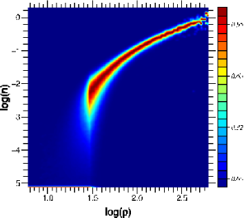
(a) $z=3$

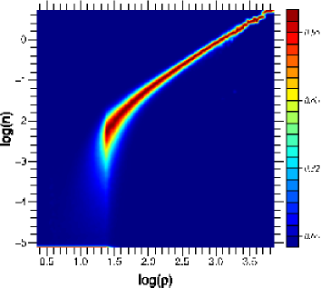
(b) $z=1$

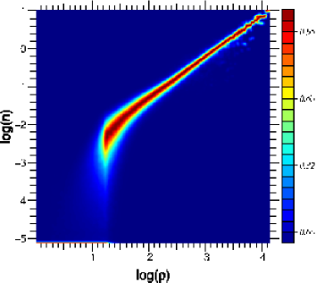
(c) $z=0$

Figure 1.— The probability $P\left(n_{G}\left|\rho_{S}\right.\right)$ that a given galaxy number density $n_{G}$ corresponds to a dark matter mass density $\rho_{S}$ for different redshifts (logarithmic scales). For low dark matter densities, no galaxy formation occur and the galaxy number density is thus $0$ whereas it appears directly proportional to the dark matter density $\rho_{S}$ for high values of $\rho_{S}$. In between this two regimes, a wide range of galaxy densities can correspond to a given dark matter density. See main text for an explanation of the change of behavior with redshift.

The function $P\left(n_{G}\left|\rho_{S}\right.\right)$ describes how the galaxy distribution maps to the underlying dark matter distribution but does not contain any information about the galaxy properties. In order to be able to attribute a spectrum to every galaxy created from $S_{l}$, we compute the probability distribution $P\left(F_{i}{\left({\lambda}\right)}\left|n_{G},\rho_{S}\right.\right)$ that a given galaxy located at point ${\bf r}$ has a given spectrum $F_{i}{\left({\lambda}\right)}$, knowing that the galaxy number density is $n_{G}{\left({{\bf r}}\right)}$ and the dark matter mass density is $\rho_{S}{\left({{\bf r}}\right)}$. This distribution is obtained from $G_{s}$ and $S_{s}$, using the $N$ synthetic spectra $F_{i}{\left({\lambda}\right)}$ generated by GalICS in $G_{s}$:

$$\left\{\begin{array}[]{l}\displaystyle P\left(F_{i}{\left({\lambda}\right)}\left|n_{G},\rho_{S}\right.\right)\propto\\ \displaystyle\;\;\;\;\;\;\;\;\;\sum_{j=1}^{N_{n}}\delta{\left({\rho_{S}{\left({{\bf r}_{j}}\right)}-\rho_{S}}\right)}\delta{\left({n_{G}{\left({{\bf r}_{j}}\right)}-n_{G}}\right)}W{\left({{\bf r}_{i}-{\bf r}_{j}}\right)},\\ \displaystyle\sum_{i=1}^{N}P\left(F_{i}{\left({\lambda}\right)}\left|n_{G},\rho_{S}\right.\right)=1.\end{array}\right.$$ (5)

In this equation, ${\bf r}_{i}$ is the location of the $i^{th}$ galaxy in $G_{s}$, ${\bf r}_{j}$ the coordinates of the $j^{th}$ grid node and $F_{i}{\left({\lambda}\right)}$ the spectrum associated to the $i^{th}$ galaxy. This simply states that the probability for a given type of galaxy to exist at a place where the galaxy and dark matter densities are $n_{G}$ and $\rho_{S}$ is proportional to the number of galaxies of that type observed in $G_{s}$ close to grid nodes, each being weighted by their respective contribution to the value of $n_{G}$ at that node (hence the factor $W{\left({{\bf r}_{i}-{\bf r}_{j}}\right)}$). From a more practical point of view, a list of spectra is attributed to every pixel in Figure 1 with a weight associated to each of them.

2.2. Generating the galaxy distribution

The first step of the process consisted of extracting information from $S_{s}$ and $G_{s}$ through the computation of probability distributions $P\left(n_{G}\left|\rho_{S}\right.\right)$ and $P\left(F_{i}{\left({\lambda}\right)}\left|n_{G},\rho_{S}\right.\right)$. The second step aims to build a galaxy distribution $G^{\star}_{l}$ out of the large scale dark matter simulation $S_{l}$ using $P\left(n_{G}\left|\rho_{S}\right.\right)$ and $P\left(F_{i}{\left({\lambda}\right)}\left|n_{G},\rho_{S}\right.\right)$. To do so, we first compute the sampled galaxy number density field $n_{G^{\star}_{l}{\left({{\bf r}_{i}}\right)}}$ corresponding to $S_{l}$. Using the same technique and grid parameters as before, the sampled mass density field $\rho_{S_{l}}{\left({{\bf r}_{i}}\right)}$ is extracted and, for every grid node $i$, a corresponding value of $n_{G^{\star}_{l}{\left({{\bf r}_{i}}\right)}}$ is randomly selected, following the probability distribution $P\left(n_{G}\left|\rho_{S}\right.\right)$.

The galaxy distribution $G^{\star}_{l}$ can then be generated by creating a point distribution whose sampled density field is $G^{\star}_{l}$. Let

$$\left\|{W{\left({{\bf r}}\right)}}\right\|=\sum_{i=1}^{N}W{\left({{\bf r}-{\bf r}_{i}}\right)}$$ (6)

be the sampled norm of the kernel $W$, with $i$ the index of a grid node. The fact that we used a truncated Gaussian kernel implies that $\left\|{W{\left({{\bf r}}\right)}}\right\|$ is not exactly constant but rather $\sigma$-periodic. It is nonetheless possible to show empirically that when $L\leq\sigma$,

$$\frac{{\rm{max}}_{\bf r}{\left({\left\|{W{\left({{\bf r}}\right)}}\right\|}\right)}-{\rm{min}}_{\bf r}{\left({\left\|{W{\left({{\bf r}}\right)}}\right\|}\right)}}{{\rm{min}}_{\bf r}{\left({\left\|{W{\left({{\bf r}}\right)}}\right\|}\right)}}\leq 1\%,$$ (7)

where ${\rm{min}}_{\bf r}{\left({f({\bf r})}\right)}$ and ${\rm{max}}_{\bf r}{\left({f({\bf r})}\right)}$ are the minimal and maximal values of $f{\left({{\bf r}}\right)}$. So as long as $L\leq\sigma$, it is possible to consider that $\left\|{W{\left({{\bf r}}\right)}}\right\|$ is a constant and the total number of galaxies $N_{G^{\star}_{l}}$ in $G^{\star}_{l}$ is:

$$N_{G_{g}^{\star}}=\frac{1}{\left\|{W{\left({{\bf r}}\right)}}\right\|}\sum_{i=1}^{N_{g}}n_{G_{g}^{\star}}{\left({{\bf r}_{i}}\right)},$$ (8)

$N_{g}$ being the total number of grid nodes.

Following the hypothesis that, on the scale at which we are working (i.e of order $1h^{-1}$ Mpc), the galaxy distribution should follow the dark matter distribution, the galaxy distribution is generated by changing dark matter particles from $S_{l}$ into galaxies or removing them following some criteria. This way, the galaxy distribution is assured to follow the large scale distribution of dark matter. Knowing the value of the galaxy number density field $G^{\star}_{l}$, the probability $Q_{i}$ for a dark matter particle to be transformed into a galaxy can be expressed as:

$$Q_{i}\propto\frac{n_{G}{\left({{\bf r}_{i}}\right)}}{\rho_{S}{\left({{\bf r}_{i}}\right)}},$$ (9)

which can be normalized using the fact that a total of $N_{G_{g}^{\star}}$ should be created:

$$Q_{i}=N_{G_{g}^{\star}}{\left({\frac{n_{G}{\left({{\bf r}_{i}}\right)}}{\rho_{S}{\left({{\bf r}_{i}}\right)}}}\right)}{\left({\sum_{j=1}{N_{S}}\frac{n_{G}{\left({{\bf r}_{i}}\right)}}{\rho_{S}{\left({{\bf r}_{i}}\right)}}}\right)}^{-1},$$ (10)

where $i$ corresponds to the index of one of the $N_{S}$ dark matter particles in $S_{l}$. For every dark matter particle, located at position ${\bf r}_{i}$, the local galaxy and dark matter densities $n_{G}{\left({{\bf r}_{i}}\right)}$ and $\rho_{S}{\left({{\bf r}_{i}}\right)}$ are linearly interpolated from the values at surrounding grid nodes, and every particle is changed into a galaxy or rejected with a probability $Q_{i}$. The attribution of a spectrum to every generated galaxy follows the same process: if a galaxy is created at a location where the galaxy and dark matter density are $n_{G}$ and $\rho_{S}$, then one of the $N_{s}$ spectra $F_{i}{\left({\lambda}\right)}$ in $G_{s}$ is attributed to it, following the probability distribution $P\left(F_{i}{\left({\lambda}\right)}\left|n_{G},\rho_{S}\right.\right)$. In the unlikely case where $Q_{i}>1$ (which means that the local galaxy number density is superior to the dark matter number density), a number of galaxies equal to the integer part of $Q_{i}$ are generated and randomly located on a sphere of radius $d$ centered on ${\bf r}_{i}$, $d$ being a random number with a probability distribution $W{\left({d}\right)}$ (i.e. identical to the kernel used for the density sampling).

3. Verifying the Galaxy distribution

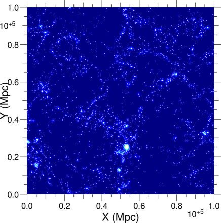
(a) GALICS256, $40h^{-1}$ slice, $30,765$ total galaxies

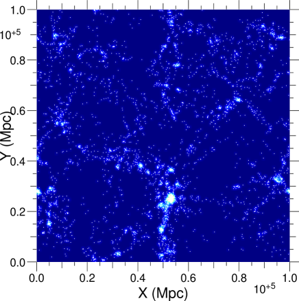
(b) MOCK256, $40h^{-1}$ slice, $30,941$ total galaxies

Figure 2.— Comparison of the two galaxy distributions obtained with GalICS and MoLUSC from the same dark matter distribution. The MoLUSC version was computed with a $1h^{-1}$ Mpc smoothing length from the dark matter simulation and its GalICS counterpart.

Using the previously described process, one can generate a large scale galaxy distribution from a large scale dark-matter-only simulation by mimicking the properties of a smaller scale galaxy distribution generated using sophisticated semi-analytical models such as GalICS. To check the quality of the results, we generated a galaxy distribution $G^{\star}$ from a $100h^{-1}$ Mpc with $256^{3}$ particles simulation $S$ using the properties of the galaxy distribution $G$ generated with GalICS from the same simulation. Figure 2(a) shows a $40h^{-1}$ Mpc slice of $G$ and 2(b) a $40h^{-1}$ Mpc slice of $G^{\star}$. In the two cases, the total number of galaxies is very similar: $30,765$ with GalICS as opposed to $30,941$ for MoLUSC. Moreover, the scheme makes the distribution very similar on scales larger than the smoothing length of $1h^{-1}Mpc$ (halos, filaments and voids are located at the same place). Nonetheless, galaxy clusters generated by MoLUSC clearly appear more spread out than the ones generated with GalICS. This is due to the Gaussian smoothing that is part of MoLUSC process. The other difference in cluster appearance is their shape but constitute this time a strength of MoLUSC. GalICS uses a spherical collapse approximation for halos such that galaxies are distributed completely spherically within a halo, but this is not necessarily the case with MoLUSC which does not require any halo identification. This results in galaxy clusters that really follow the underlying matter distribution, thus presenting different geometries.

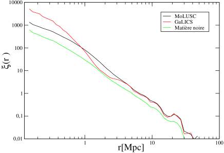
Figure 3.— Two-point correlation function $\xi(r)$ of the dark matter distribution (green curve) and of the galaxies distributions generated by GalICS (red curve) and MoLUSC (black curve). The smoothing length used for MoLUSC is $L=1h^{-1}$ Mpc. Part of the particles in the dark matter simulation have been randomly removed so that the number of points is the same.

The examination of the two point correlation functions $\xi{\left({r}\right)}$ in Figure 3 confirms the preceding remarks. MoLUSC mainly aims to reproduce GalICS galaxy distribution. The comparison of the correlation functions for $G$ (red curve) and the one for $G^{\star}$ (black curve) indicates that they are similar on scales larger than $2h^{-1}$ Mpc while some differences exist on smaller scales. It is clear that below scales of order the smoothing length ($1h^{-1}$ Mpc here), correlations are weaker with MoLUSC in which case they tend to follow the dark matter correlation function (green curve). Between scales of order the smoothing length and $2h^{-1}$ Mpc, the opposite situation appear: whereas correlations are lacking in $G$ because of the spherical halo model used by Galics, this is not the case in $G^{\star}$. All these observations tend to show that MoLUSC is particularly appropriate for the production of large scale distributions of galaxy out of a large scale dark matter-only simulation.

4. Real space snapshot to redshift catalog conversion

Once the simulation has been populated with galaxies, the primary difference remaining between a simulation and a survey like SDSS is that observing galaxies introduce biases that are not present in a simulation. So now that we have obtained a galaxy distribution, there is still to make a mock catalog emulating these biases. First of all, when galaxy properties are measured with a telescope, one often only measures their redshift and their apparent magnitude in a given filter. All other properties like the absolute magnitude or distance has to be computed from these values. This of course introduce errors and limitations, the main ones being that:

1. The spectrum of a galaxy is not constant with wavelength. So as it is redshifted because of the expansion of the universe, the apparent magnitude is not measured in the same wavelength range as the absolute magnitude. This can be corrected by using so called K-corrections, the value of which depends on galaxy morphology, redshift and filter characteristics.

2. The measured redshift is used to compute a distance assuming it is only due to the expansion of the universe. The peculiar velocities are neglected in the process and give rise to so-called redshift distortions and the “finger of god” effect.

3. The geometry of a survey is constrained by practical matters, giving rise to complex geometry as seen with SDSS on fig 5.

Some aspects of the procedure used are quite similar to the one described in Blaizot et al. (2005). The reader can refer to this paper for further details on some points.

To build a more realistic mock catalog, we can also take into account incompleteness with distance, the zone of obscuration and one could imagine to add a surface brightness selection since the absolute luminosity is available from the simulations.

4.1. Basic equations

For a given cosmological model, the comoving distance between a galaxy at redshift $z$ and an observer in a flat universe can be defined as follows:

$$D(z)=\frac{c}{H_{0}}\int_{0}^{z}\frac{dz}{\sqrt{\Omega_{m}(1+z)^{3}+\Omega_{\phi}f(z)}},\;\;\;\Omega_{m}+\Omega_{\phi}=1$$ (11)

where $\Omega_{m}$ and $\Omega_{\phi}$ are the fraction of matter and dark energy respectively. The function $f(z)$ depends on the cosmological model. If we consider the $\Omega_{\phi}$ part to be modeled by a fluid with an equation of state $p=w\rho$ then we obtain

$$f(z)=(1+z)^{3(1+w)},\;\;\;p=w\rho$$ (12)

which gives $f(z)=1$ in the case of a LCDM model. The distance (11) is not directly observable, but corresponds to the distance than one can measure directly between two galaxies in a simulation box. It can be easily related to luminosity distance by $d_{L}=(1+z)D$ where $d_{L}$ is the luminosity distance.

Although Equation 11 is not analytically solvable in the general case, a low redshift approximation can be used for our purpose, giving at second order in $z$:

$$D(z)=\frac{c}{H_{0}}\left(z-\frac{1}{2}\left(1+q_{0}\right)z^{2}\right)$$ (13)

with $q_{0}$ the deceleration parameter:

$$q_{0}=\frac{\Omega_{m}}{2}+\frac{\Omega_{\phi}}{2}\left(1+3w\right).$$ (14)

Finally the classic relationship between apparent and absolute magnitude is given by:

$$M=m-5\log\left(D(z)(1+z)\right)-25+K(z)$$ (15)

where $D(z)(1+z)=d_{L}$ is the luminosity distance, $M$ the absolute magnitude, $m$ the apparent magnitude and $K(z)$ stands for the K-correction term.

4.2. Mock catalog construction

One of the major problems of studies of large-scale structure is that it is quite difficult to compare theoretical results to observational data in a fair way. With MoLUSC, one can generate a large scale galaxy distribution from a dark matter only simulation. Galaxies, being generated from an N-body simulation, are distributed in a series of data cubes representing universe snapshots at different redshifts. A galaxy catalog such as SDSS is different in that it represents the galaxy distribution as viewed by an observer. Thus, making mock catalogs consists of reproducing from the data cubes a galaxy distribution similar to what would be observed, taking into account all the observational biases.

Initially, every snapshot contains the following information:

• The value of the redshift.

• The location and velocities of all galaxies.

• For every galaxy, a corresponding spectrum.

By randomly placing an observer within the $z=0$ snapshot, and defining a line of sight direction, it is possible to compute the observational properties of the galaxies belonging to the volume of the galaxy catalog to mimic, paying attention to the fact that the galaxies should be extracted from the snapshot with redshift corresponding to the distance between the observer and the galaxy. The main problem with this method is that the original simulation can be smaller in size than the galaxy catalog for which a mock catalog is being generated. Of course, one benefit of the MoLUSC technique is that very large galaxy distributions can be easily generated, but still it can be that every snapshot has to be duplicated in order to obtain a distribution on a large enough volume. This technique is called random tiling and consists of stacking simulation snapshots after applying to each of them random rotations and translations, using the periodic boundaries condition to ensure that the transformed snapshots have the same geometry. The random transformations are very important in that they prevent the final distribution from being periodic as anyway no information exists on scales larger than that of the snapshots.

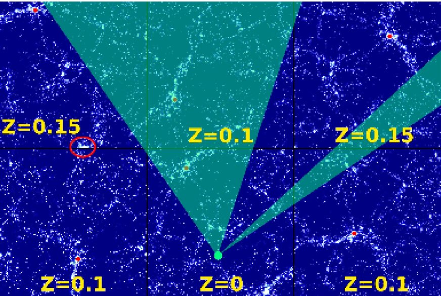
Figure 4.— Illustration of the random tiling method and of the construction of mock catalogs from the initial catalogs. The space is made from initial catalogs with different redshifts which have been randomly transformed (rotation, translation). The red dots show the same cluster of galaxies. The red circle illustrates the problem of clusters lying close to a side of a box. To create a mock catalog, only the galaxies included in the geometry of the initial catalog (here in green) are selected.

Figure 4 illustrates the random tilling method. The main drawback comes from the fact that a large cluster can be cut if it is located at a place where the snapshot used to build the mock catalog changes. This problem is solved using a friends-of-friends type structure finder: instead of computing observational properties of the galaxies one by one, it is done for every cluster and depending on the cluster center position, all of its galaxies will be present or absent of the mock catalogs. The influence of random tilling on the correlation function can be found in Blaizot et al. (2005), section 3.

4.3. Final catalogs

Galaxy catalogs often have complex geometries due to observational constraints. It is important to reproduce them in order to be able to check the influence of edge effects. To do so, the method we use simply consists of building a mask from the real catalog and applying it to the mock catalog. Once the catalog is built, the only step left involves reproducing the main observational biases: redshift distortions and spectral redshifting. Redshift distortions are taken into account by using the peculiar velocities of the galaxies obtained from the simulation snapshots. To a galaxy at a given distance we add a redshift due to hubble flow to an additional term due to the peculiar velocity that prevents an exact distance measurement. The amplitude of this term is simply given by:

$$\delta z=\sqrt{\frac{1+{\bf v}_{p}}{1-{\bf v}_{p}}}-1$$ (16)

where ${\bf v}_{p}$ is the norm of the peculiar velocity projection on the line of sight. Finally, the galaxies’ absolute and apparent magnitudes are computed using GalICS synthetic spectra as observed through a given filter $F{\left({\lambda}\right)}$. This way, the $i^{th}$ galaxy with redshift $z_{i}+\delta z_{i}$ with a rest frame spectrum $P_{i}{\left({\lambda}\right)}$ has an observer frame spectrum:

$$P^{\rm{obs}}_{i}{\left({\lambda}\right)}=\frac{P_{i}{\left({\lambda{\left({1+z_{i}}\right)}}\right)}}{1+z_{i}},$$ (17)

and its absolute and apparent magnitudes $M_{i}{\left({F}\right)}$ and $m_{i}{\left({F}\right)}$ are:

$$M_{i}=\int_{0}^{\infty}P_{i}{\left({\lambda}\right)}F{\left({\lambda}\right)}\,d\lambda$$ (18)

and

$$m_{i}=\int_{0}^{\infty}P^{\rm{obs}}_{i}{\left({\lambda}\right)}F{\left({\lambda{\left({1+z_{i}}\right)}}\right)}\,d\lambda.\\$$ (19)

Figure 5 shows the result obtained for a mock SDSS DR4 catalog using MoLUSC with different observational biases taken into account.

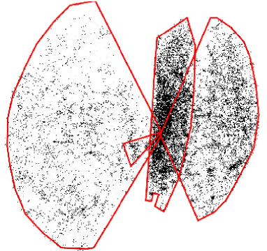
(a) DR4-350

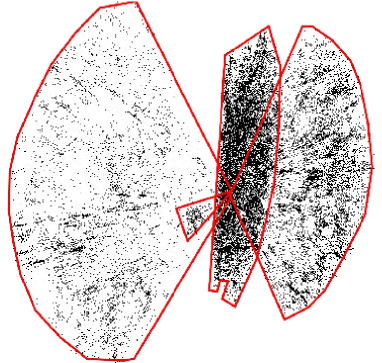
(b) MOCK

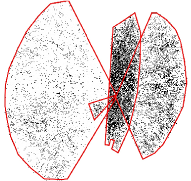
(c) MOCK-NB

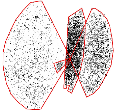
(d) MOCK-NBNF

Figure 5.— Comparison between the observed SDSS DR4 (a) survey (limited to 350 Mpc) and 3 different virtual SDSS surveys (b, c, d) built from the large scale low resolution DM simulation. The virtual catalog MOCK (b) is made taking into account all the observed selection effect and observational artifacts as the fingers of god. The MOCK-NB (c) is built while neglecting the bias between galaxies and DM. This results in a less contrasted density field. In MOCK-NBNF (d) both the bias and the redshift distortions were not accounted for. As a result of this lack of observational artifacts the galaxy clusters appear almost sphericals, not elongated along the line of sight.

5. Conclusions

In this paper we presented MoLUSC, a tool for extracting mock galaxy surveys out of large scale pure dark matter numerical simulations. Our method consists of first computing numerically at a given redshift how the galaxy distribution maps to the underlying dark matter distribution using a high resolution small scale simulation. We are then able to reproduce the galaxy distribution characteristics from a snapshot of any size and resolution, while conserving proper statistical properties.

Galaxy properties are computed as measured by an observer. Bias effects such as fingers of god, k-corrections on magnitudes, catalog geometry are numerically computed allowing a fair comparison to the observed data which is crucial in order to study the formation and evolution of the large-scale structures in the Universe.

MoLUSC is being used to provide mock catalogs of the SDSS and of the Deep Fields of CFHTLS, for a variety of cosmologies. The observers are provided with mock catalogs matching the survey selection effects such as magnitude depth and survey geometry. The virtual observations are provided in the corresponding survey set of filters.

This tool provides a realistic galaxy distribution out of any large dark matter only simulation without using powerful computer hardware, allowing a faster astrophysical analysis of the present large DM simulations.

References

- Blaizot et al. (2005) Blaizot J., Wadadekar Y., Guiderdoni B., Colombi S.T., Bertin E., Bouchet F., Devriendt J.E.G., Hatton S., 2005, MNRAS, 360, 159
- Cole et al. (1998) Cole, S., Hatton, S., Weinberg, D. H., & Frenk, C. S. 1998, MNRAS, 300, 945
- Hamana et al. (2002) Hamana, T., Colombi, S. T., Thion, A., Devriendt, J. E. G. T., Mellier, Y., & Bernardeau, F. 2002, MNRAS, 330, 365
- Hatton et al. (2003) Hatton S., Devriendt J.E.G., Ninin S., Bouchet F.R., Guiderdoni B., Vibert D., 2003, MNRAS, 343, 75-106
- Jing et al. (1998) Jing, Y. P., Mo, H. J., & Boerner, G. 1998, ApJ, 494, 1
- Peacock & Smith (2000) Peacock, J. A., & Smith, R. E. 2000, MNRAS, 318, 1144
- Springel et al. (2001) Springel V., Yoshida N., White S. D. M., 2001, New Astronomy, 6, 51
- Springel (2005) Springel V., MNRAS 2005, 364, 1105
- Yan et al. (2003) Yan, R., Madgwick, D. S., & White, M. 2003, ApJ, 598, 848
- Zhao et al. (2002) Zhao, D., Jing, Y. P., Börner, G. 2002, ApJ, 581, 876