Late-Time Convection in the Collapse of a 23 Solar Mass Star

Abstract

The results of a 3-dimensional SNSPH simulation of the core collapse of a 23 M_⊙ star are presented. This simulation did not launch an explosion until over 600 ms after collapse, allowing an ideal opportunity to study the evolution and structure of the convection below the accretion shock to late times. This late-time convection allows us to study several of the recent claims in the literature about the role of convection: is it dominated by an $l=1$ mode driven by vortical-acoustic (or other) instability, does it produce strong neutron star kicks, and, finally, is it the key to a new explosion mechanism? The convective region buffets the neutron star, imparting a $150-200{\rm\,km\,s^{-1}}$ kick. Because the $l=1$ mode does not dominate the convection, the neutron star does not achieve large ($>450{\rm\,km\,s^{-1}}$) velocities. Finally, the neutron star in this simulation moves, but does not develop strong oscillations, the energy source for a recently proposed supernova engine. We discuss the implications these results have on supernovae, hypernovae (and gamma-ray bursts), and stellar-massed black holes.

1 Introduction

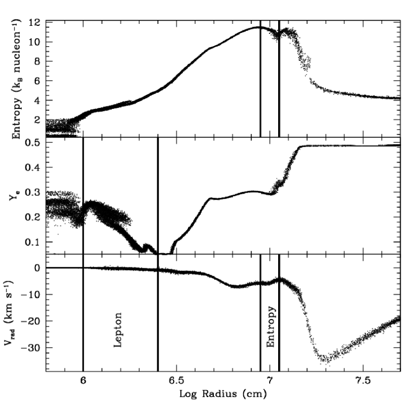
Figure 1: Entropy (top), Electron Fraction (Middle), and Radial Velocity (bottom panel) as a function of radius for our simulation 50 ms after bounce (roughly at the time of the stall of the bounce shock). We see that a negative lepton gradient has developed near the neutrinosphere. It is this initial gradient that leads to convection within the proto-neutron star. Beyond the neutron star, just below the accretion shock, we see the initial negative entropy gradient that initially drives the convection in this outer region. At this time, with this low resolution simulation, no strong convection has developed, but these are the two regions in which we expect convection to occur.

Since Epstein (1979) first proposed that convection could increase the neutrino luminosity arising from newly formed neutron star, core-collapse theorists have studied the potential roles convection may play in the supernova explosion mechanism. This work has identified 2 different regions where instabilities are produced: (1) within the proto-neutron star and (2) the region between the accretion shock and the outer surface of the proto-neutron star (Fig. 1). Convection within the proto-neutron star originates initially from the lepton gradients near the neutrinosphere as proposed by Epstein, but the convective instabilities that grow involve much more complex criteria than simple weight gradients (Keil et al. 1996, Bruenn et al. 2004). If the convection can grow, it can help transport neutrinos out of the core, effectively increasing the luminosity of neutrinos at early times. The strength of this convection is still an important topic of study and it remains to be seen if this convection grows beyond the limited region near the neutrinosphere: indeed, most simulations (either rightly or wrongly) do not exhibit strong proto-neutron star convection (e.g. Herant et al. 1994; Fryer & Warren 2002; Buras et al. 2003). The role of this convection can only be answered with a detailed knowledge of the equation of state at nuclear densities (Bruenn et al. 2004).

On the other hand, convection above the proto-neutron star tends to be strong in most multi-dimensional models (e.g. Herant et al. 1994; Burrows et al. 1995; Mezzacappa et al. 1998; Fryer & Warren 2002; Buras et al. 2003; Burrows et al. 2006). This convection, initially driven by the entropy gradient left behind after the stall of the bounce shock aids the conversion of heat released by gravitational potential energy during the infall into kinetic energy of an explosion (see Fryer 2003 for details). One of the debates with this convection is the role it plays in helping to drive an explosion. Herant et al. (1994) focused on the role convection played in transporting the neutrino-heating material out of the star allowing this thermal energy to convert to kinetic energy. The convective region is also a resevoir for the energy “useful” energy, that is, energy that can drive an explosion. But until recently, the effect of this convection met with mixed results where some multi-dimensional simulations achieved strong explosions due to convection and others produced no explosion whatsoever (compare Herant et al. 1994 to Mezzacappa et al. 1998). But as we shall discuss below, there is a growing consensus that this convective region is important in core-collapse supernovae. Indeed, convection has been recently proposed as not just an aid in converting neutrino heat energy into an explosion, but as the primary means of generating the energy behind the supernova explosion (Burrows et al. 2006).

Another growing debate surrounding the convective region above the proto-neutron star focuses on the cause of this instability. Herant et al. (1994) originally focused on the entropy gradient set by the stall of the bounce shock and the entropy generated by neutrino heating at the base of this convective region. Shock heating produced by the downflows as they strike the hard surface of the proto-neutron star also contributes to the convective instability of the region. Blondin et al. (2003) focused their analysis on the instabilities produced at the top of this convective region, also termed accretion shock instabilities. Due to the low-mode nature of their convection, they argued for a new (third) type of instability extracting the energy stored in vorticity and converting this energy into sound waves, the “voritical-acoustic” instability. Although this instability has attracted the attention of additional supernova groups (e.g. Burrows et al. 2006), Blondin & Mezzacappa (2006) remain prudently wary (if not doubtful) of their own proposal, focusing instead on the more classical drivers behind accretion shock instabilities (Houck & Chevalier 1992). But Burrows et al. (2006) have found that this vortical-acoustic instabilities drove oscillations in the proto-neutron star that ultimately can power a supernova explosion.

Convection above the proto-neutron star may also be the cause of the strong kicks observed in the pulsar population and required to explain a number of binary systems (see Fryer et al. 1998 and Lai et al. 2001 for reviews). Herant (1995) used the simulations of Herant et al. (1994) to argue that if such modes merged, a strong kick could be produced. Scheck et al. (2004) have now run a series of simulations showing that such a kick mechanism is not only plausible, but can also produce the obvserved pulsar velocity distribution.

It is difficult to compare/contrast this large set of multi-dimensional core-collapse calculations. Core-collapse is a complex problem, with a wide range of physics that can play an important role in the development of the explosion. Different calculations have different implementations (with varying levels of sophistication) of this physics. Many of these results are based on 2-dimensional simulations with simplified treatments of the neutron star. Others do not model convection out to late times, an important factor in the development of low mode convection. In this paper, we present the results of the collapse of a 23 M_⊙ star, following the convection $\sim$400 ms after bounce (over 600 ms after the collapse of the massive star). In §2, we discuss the code used in these calculations and its strengths and weaknesses versus other techniques. §3 focuses on the convective region above the proto-neutron star and the evolution of this convection with an effort to distinguish between numerical and real results. §4 moves this study inward to the motion and evolution of the proto-neutron star. We conclude with a discussion of the implications of these results on our current understanding of supernovae.

2 Initial Conditions and Numerical Techniques

Our initial progenitor is a 23 M_⊙ star produced by the Tycho stellar evolution code (Young & Arnett 2005). The Tycho code itself is evolving away from the classic technique (mixing-length theory) of modeling convection to a more realistic algorithm based on multi-dimensional studies of convection in the progenitor star (Meakin et al. 2005). In Figure 2 we see that the density and entropy structure of this progenitor is quite different than those produced by classic stellar evolution codes such as Kepler (Heger et al. 2006). One key difference is the lack of jumps in the density and temperature profile in the star produced using the Tycho stellar evolution code. The jumps are an artifact of mixing length theory, which ignores hydrodynamic tranport processes at and outside of the convective boundary. In shell burning especially, inner convective boundaries are stiff, but outer boundaries are soft. Due to the large bouyancy frequencies at the boundary, relatively low mach number flows ($M\sim 0.01$) can generate waves in the intershell regions with density contrasts of $\delta\rho/\rho$ of order 10% in oxygen burning (Meakin & Arnett 2006b). These processes smooth the temperature and density gradients. More realistic treatment of the convective and boundary hydrodynamics also results in larger convective zones. The differences in the structure will affect the fate of the star, and it is likely that uncertainties in the progenitor dominate the uncertainties in any core-collapse calculation. We also compare this structure to the structure of the classic 15 M_⊙ progenitor (s15s7b2: Woosley & Weaver 1995) used as a standard in many core-collapse calculations. Note that higher mass stars have cores with higher entropies. The 23 M_⊙ progenitor used in this study is produced with a version of the Tycho code part way through this transformation, and we expect the exact structure of this 23 M_⊙ to change as stellar evolution codes improve (although preliminary results suggest the changes with the fully transformed code will be small - Young, pvt. communication).

The higher densities in the 23 M_⊙ models over the 15 M_⊙ star lead to higher accretion rates (and a higher ram pressure) at the top of the convective region. It is this infalling material that prevents the supernova explosion (Fryer 1999). Figure 3 shows the accretion rates for the 3 progenitors: the 23 M_⊙ in this study from Tycho (Young & Fryer 2006), a 23 M_⊙ Kepler model (Heger et al. 2006), and the 15 M_⊙ standard model (Woosley & Weaver 1995). The 23 M_⊙ models have a higher accretion rate, and hence higher ram pressure to overcome to drive a supernova explosion. Here is where the difference between stellar evolution codes truly stands out. Note the large difference between accretion rates. The difference between the Kepler and the Tycho 23 M_⊙ is nearly as large as the difference between a Kepler 23 M_⊙ and a Kepler 15 M_⊙ star. Unfortunately, the sharp boundaries in the Kepler models made it easy to predict the explosion energy or time (Fryer 1999). Without these, estimating these explosion parameters becomes much more difficult.

When our progenitor begins to collapse, we map the 1-dimensional star into a 3-dimensional smooth particle hydrodynamics setup. The particles are added in a series of shells, where the number of particles in each shell is determined by the density in the 1-dimensional progenitor and the mass of the particles. The particle masses are identical within each shell, but vary from shell to shell in order to put the highest resolution in the inner portion of the star near the action. In each shell, the particles are placed in random, but equally separated positions (see Fryer et al. 2006a for details). Although this randomness prevents any preferred direction in the collapse, it does lead to density perturbations in the initial model. These density perturbations can be seen in an early time dump of the collapsing star. At high resolution, we can minimize these pertubations, but for our low-resolution simulation, the magnitude of the pertubation can become quite high. We have lowered the tolerance in the setup code to minimize this perturbation. Even so, the initial density perturbation of this low-resolution calculation is $\sim$3-5%. Note that this value is close to what we expect from multi-dimensional models of the progenitors (Bazan & Arnett 1998, Meakin & Arnett 2006a). But our perturbations our not correlated, and the multi-dimensional models predict more correlated perturbations. A correlated perturbation will likely produce an initial convective profile that is more asymmetric than our small-scale perturbations. The larger asymmetries might lead to a stronger initial convection and more mixing in the ejecta of the explosion.

We chose a low resolution to delay the growth of convection. It has long been known that the SPH calculations by Herant et al. (1994) and subsequent papers by Fryer and collaborators (e.g. Fryer & Warren 2002) tend to develop strong convection earlier than models using grid techniques. Fryer & Kusenko (2006) found that by limiting the resolution, this delay can be mimicked in the SPH calculations. Hence, the resolution is set to 500,000 particles for the entire 5.6 M_⊙ stellar core modeled in our calculation. We will discuss the growth time of convection in more detail in the next section (where we argue that the short delay in high-resolution SPH calculations is actually closer to reality than those calculations with delayed convection).

We use the SNSPH code (Fryer et al. 2006a) to follow the collapse, convective, and ultimately explosion phase of this model. This code has passed several tests of its gravity routine. Especially in modeling the convective region when the neutron star begins to move, it is important that this gravity routine be accurate. The fact that SNSPH is a gridless technique also makes it an ideal code for studying neutron star motions, as no numerical issues arise when the neutron begins to move.

SNSPH transport has been compared to 2-dimensional and 1-dimensional flux-limited diffusion schemes. But its neutrino transport is still limited to a 3-flavor, single-energy flux-limited diffusion algorithm. Such a scheme is believed to increase the net neutrino heating, making an explosion easier. Although the equation of state can couple an accurate nuclear-statistical equilibrium algorithm (Hix & Thielemann 1996) to the Lattimer-Swesty (1991) equation of state for neutron star matter (see Herant et al. 1994 for details), to better compare to the work of other authors, we use the Lattimer-Swesty equation of state down to densities of $10^{9}{\rm\,g\,cm^{-3}}$. Because of the incorrect energy levels in the Lattimer-Swesty algorithm for nuclear statistical equilibrium, this choice alters significantly the entropy profile of the convective region with our models (see Fryer & Kusenko 2006) .

Smooth particle hydrodynamics is a Lagrangian code, and SNSPH uses the standard artificial viscosity algorithm seen in many Lagrangian codes to model shocks. It tends to not model shock fronts as well as a grid code using the piecewise parabolic method can do (at least as long as the shock is traveling along the grid - see Fryer et al. 2006a for details). Also, this artificial viscosity is generally larger than the true viscosity in core-collapse problems (at least those without magnetic fields), effectively lowering the Reynolds number of our numerical calculation. This damps out high-order modes in any convective instability. We will discuss this effect in more detail in the next section.

3 Convective Instabilities

50 ms after bounce, an entropy gradient has developed just behind the accretion shock (Figure 1). Such an entropy gradient is extremely susceptible to Rayleigh-Taylor convection. One way to estimate the timescale of this convection is to use the Brunt-Väisäla frequency $\omega$ (see Cox, Vauclair, & Zahn 1983):

$$\omega^{2}=g/\rho(\partial\rho/\partial S)_{\rm P}(\partial S/\partial r)$$ (1)

where $\rho,S$ are the density, entropy of the matter, $(\partial\rho/\partial S)_{\rm P}$ is the partial derivative of the density with respect to entropy at constant pressure, $(\partial S/\partial r)$ is the partial derivative of the entropy with respect to the radius $r$ of that matter and $g\equiv GM_{\rm enclosed}/r^{2}$ is the gravitational acceleration. Here $G$ is the gravitational constant and $M_{\rm enclosed}$ is the enclosed mass at radius $r$. If $(\partial S/\partial r)$ is negative, $\omega^{2}$ is negative and the region is unstable. The timescale for this convection ($\tau_{\rm conv}$) is $(|1/\omega^{2}|)^{1/2}$.

In the limit where radiation pressure dominates the pressure term (reasonably true at the accretion shock), this equation becomes:

$$\omega^{2}=g/S(\partial S/\partial r)\approx(1/S)(GM_{\rm enclosed})/r^{2})(\Delta S/\Delta r)$$ (2)

where $\Delta S$ is the change in entropy over distance $\Delta r$. Here we used the following relations: $S\propto T^{3}/\rho$ and ${\rm Pressure}\propto T^{4}$. For the conditions in Fig. 1, where $g\approx 1.5\times 10^{12}\,{\rm cm\,s^{-2}}$, $\Delta S/S\approx 0.2$, and $\Delta r\approx 10^{7}{\rm cm}$, the convective timescale is roughly 2 ms. Even on core-collapse timescales, this is extremely rapid. It is worth noting that the negative entropy gradients in models using a modified equation of state (Herant et al. 1994, Fryer & Kusenko 2006) have much larger amplitudes, leading to even more rapid growth of convection.

Some scientists prefer to estimate the growth time of Rayleigh-Taylor instabilities based on a more simplified equation using the Atwood number $A$:

$$\omega_{\rm Atwood}^{2}=kgA$$ (3)

where $A=(\rho_{2}-\rho_{1})/(\rho_{2}+\rho_{1})$ and $k$ is the wave number. Such an equation is designed for simplistic examples of a two density fluid chamber. But, if we again assume a radiation pressure dominated gas, this equation becomes:

$$\omega_{\rm Atwood}^{2}=k(GM_{\rm enclosed})/r^{2})(\Delta S/S).$$ (4)

If we pick a wave number roughly of the size scale of our convective region, this equation is identical to our equation derived using the Brunt-Väisäla frequency.

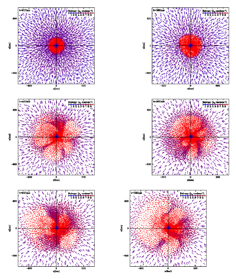
Figure 4: 6 snapshots in time of the convection in our collapsing model. We plot slices of the data in the x-z plane. The vectors denote direction and magnitude of the particle motion. The colors denote entropy. Probably because of our low resolution, the growth time is longer than we would expect from an instability analysis. But convection does develop, ultimately producing a weak explosion. The convection also is far from symmetric, but we do not get the single-sided downflows seen in many recent 2-dimensional calculations.

Figure 4 shows a time series with 6 snapshots of the convection in our collapse core. At 310 ms, 10 ms after the time in Figure 1, we see that no vigorous convection has yet to develop. 50 ms later, this convection is strong and reaches beyond 200 km. The delay (beyond the 2 ms prediction of perturbation analysis) in this convection could be because our rough estimate we obtained from equation 2 underestimated the timescale of convection, but it is more likely that numerical viscosity from this low-resolution calculation is damping the growth of the instabilities. Fryer & Kusenko (2006) found they could delay the convection by pushing towards low resolution. Fryer & Kusenko (2006) artificially prevented an explosion by using low resolution to prevent the explosion. In this paper, we focus our study on late-time convection. To ensure this, we use both a more massive progenitor, but also take advantage of the Fryer & Kusenko (2006) result and use low resolution to delay the convection and, ultimately, the explosion. We are intentionally damping the convection to allow us to study late-time convection.

Smooth particle hydrodynamics is not the only numerical hydrodynamics technique that suffers from large numerical viscosity and it is likely that the resolution (or lack thereof) in this calculation is causing the delay in the convection. Eulerian codes can also suffer from numerical damping of convection through advection (Fryer et al. 2006c, Schmidt et al. 2006).

3.1 Understanding Low-Mode Convection

Based on the low-mode convection from the Herant et al. (1994) 2-dimensional simulations, Herant (1995) argued that in the extreme case where the modes ultimately merged to produce convection along a single mode could produce asymmetric explosions and neutron star kicks. However, subsequent SPH calculations never developed single mode convection (Fryer 1999, Fryer & Warren 2002, Fryer & Warren 2004, Fryer 2004, Fryer & Kusenko 2006) unless some initial asymmetry (neutrino-driven kick, asymmetry in the progenitor, rotation) was placed on the collapse to seed this $l=1$ mode. However, recently, a number of simulations exhibit strong $l=1$ structures (Blondin et al. 2004,2006; Scheck et al. 2004; Burrows et al. 2006). Although these simulations argue for this low-mode convection, we have yet to put together a complete picture of the physics affecting this convective region. As such, it remains difficult to extract the numerical effects from those effects of a true physical nature. There exist a number of similarities between the convective instabilities in the core-collapse problem with those of Bondi-Hoyle-Littleton accretion (see Foglizzo et al. 2005 and references therein) and, already, this knowledge is being applied to the core-collapse problem.

What we do know is that there are many possible drivers behind this convection. First and foremost, as we showed above, the entropy profile in the convective region is extremely unstable to Rayleigh-Taylor instabilities. If the accretion shock capping this region moves outward, the entropy gradient will continue to be produced simply because the entropy jump at the shock decreases as the shock moves outward (Houck & Chevalier 1991, Fryer et al. 1996). Neutrino heating (and shock heating as the downflows strike the proto-neutron star) from below also serves to maintain the entropy gradient and drive Rayleigh-Taylor convection. Herant et al. (1994) focused their discussion on this convective instability. One would expect such convection to produce bubbles with sizescales roughly on the radial extent of the convective region ($\sim r_{\rm outeraccretionshock}-r_{\rm proto-neutronstar}$). When the region is small, we expect many downflows and upflows. As the convective region pushes the accretion shock outward, the number of downflows should decrease. It is this trend that we see in our simulations (Fig. 4).

A second instability has been studied by Blondin et al. (2004,2006), focusing on the accretion instability caused by spherical accretion. This instability tends to drive low order $l=0,l=1$ modes and Blondin et al. (2006) found that such modes do dominate in conditions where Rayleigh-Taylor convection is not strong. It is interesting to note that this spherical accretion shock instability was discussed in detail by Houck & Chevalier (1992) to study accretion onto neutron stars. Fryer, Herant, & Benz (1996) modeled this accretion in 2-dimensions and found that the Rayleigh-Taylor instabilities set up by the entropy gradient produced as the accretion shock moved outward again dominated the instabilities. They found that $l=$few, not $l=0$ or $l=1$, modes dominated the convection at early times. $l=$ few modes is what one expects from Rayleigh-Taylor convection and Fryer et al. (1996) believed this dominated the convection. In our collapse simulation, we might also expect that Rayleigh-Taylor convective instabilities to dominate the matter motion at early times. But as the convection persists, we see the development of an $l=1$ mode that is probably caused by the accretion shock instability studied by Blondin & Mezzacappa (2006). It appears that a combination of these two instabilities can explain the matter motion in our simulation.

A third instability, originally highlighted by Blondin et al. (2004) has also piqued the curiosity of the core-collapse community: the vortical-acoustic instability. This instability, which takes the vorticity pulled down in the downflows and converts it to sound waves, drives low-mode convection. Although Blondin & Mezzacappa (2006) now believe the instabilities they see are not the vortical-acoustic instability, new adherents (e.g. Burrows et al. 2006) have brought continued support to this particular instability. Foglizzo et al. (2006), Ohnishi et al. (2006) and Yamasaki & Yamada (2006) have also studied the relative importance of this instability. Ohnishi et al. (2006), in particular, pointed out that the relative importance of these shock instabilities will depend upon exact conditions in the models and might vary for different progenitors. The convection in our calculations can either be explained by Rayleigh-Taylor plus this vortical-acoustic instability, or by Rayleigh-Taylor plus late-time accretion shock instabilities argued by Blondin & Mezzacappa (2006).

In addition to differences in progenitors, which of these instabilities dominate in actual calculations may well be a reflection of numerical technique and not what nature produces. As an example of the role of numerics, let’s analyze the laminar nature of our downflows. In our calculations, we set the the SPH viscosity parameters $\alpha,\beta$ to 1.0,2.0 respectively. With our low resolution calculation and the velocities of and sound speeds in the downflows, we find that our numerical Reynolds number is $\sim 15$. Fryer & Warren (2004) did produce one simulation where the Reynolds number was closer to 100, but no SPH calculation of core-collapse supernovae has modeled significantly higher Reynolds numbers. As such, we expect all of our simulation to exhibit laminar flows, and they do. If convection is important in the supernova explosion, we must make sure that our numerical models match the conditions in nature.

What do we expect from nature? If the viscosity is dominated by the Spitzer viscosity (Braginskii 1958, Spitzer 1962), then the Reynolds number is many orders of magnitude higher than what we model. If this were the only viscosity, then nature would produce turbulent flows and the entire structure of the convection would be different. Currently, most simulations exhibit laminar (or close to laminar flows). Either these simulations, like our SPH simulations, have enough numerical viscosity to effectively be modeling laminar flows, or some other real viscosity is playing a role in reducing the Reynolds number. It is possible that magnetic fields can add viscosity and effectively reduce the Reynolds number, but most collapse simulations to date do not include magnetic fields (Simon 1949, Spitzer 1962).

Colgate (pvt. communciation 1996) suggested that neutrinos could increase the viscosity. Recall that the zeroth order Spitzer viscosity is given by:

$$\eta^{e}_{0}\propto nk_{\rm Boltz}T_{e}\tau_{e}$$ (5)

where $n$ is the number density, $k_{\rm Boltz}$ is the Boltzmann constant, $T_{e}$ is the electron temperature and $\tau_{e}$ is the collision time of the electrons:

$$\tau_{e}\propto T_{e}^{3/2}/(n\lambda)\,{\rm s}$$ (6)

where $\lambda$ is the Coulomb logarithm. This gives us the familiar $T^{5/2}$ dependence of the Spitzer viscosity. Let us understand this viscosity term a little bit better. The viscosity is essentially determined by the ability for the electron/ion/particle to transport momentum. This depends upon 2 factors: (1) how much momentum the particle contains (the specific energy is the specific momentum squared) and (2) how far the particle transports this momentum. If there is not much energy in the particles, they do not contribute much to the viscosity. If the particle does not move significantly before losing its preferred direction, it also does not contribute much to the viscosity. This latter effect is what reduces the contribution from electrons to the viscosity and this is why we expect a large Reynolds number if we constrain ourselves only to the the electron viscosity. Colgate’s idea was that the neutrinos, while trapped at the base of the convection, have a much longer collision time than the electrons. Using the above equations to estimate the viscosity from neutrinos (with roughly 1-10% the energy stored in electrons, but with a collision time that can be 10 orders of magnitude longer than electrons), we find that the neutrino viscosity can reduce the Reynolds number in our simulated downflows down to 1000 (and perhaps 100). For such cases, laminar-like flows are expected. But such features must be checked in every simulation.

Numerical versus real viscosity is just one example of how we have to be careful to distinguish between the results of our simulations and what is actually happening in nature. As convection plays a larger role in understanding supernovae, real versus numerical becomes a very important question that must be addressed. In the case of our current simulation, the laminar flows may well be real and the nature and evolution of the convection can be understood by our understanding of Rayleigh-Taylor and accetion shock instabilities. We do know that the dominant modes of the convection are set by the driving forces, which is not too dependent on the Reynolds number. The coherence of the flows would be changed by the onset of turbulence, but this might be a minor effect on the supernova engine. But we are also certainly seeing numerical delays on the onset of convection and the numerical viscosity in the code is setting the Reynolds number of the calculation. Fryer & Kusenko (2005) claim that these numerical delays are very important and comparing their results with with the Fryer & Warren 2002 results, this statement, as far as smooth particle hydrodynamics simulations are concerned, is true. Whether or not such numerical artifacts are affecting Eulerian calculations awaits convergence study calculations done by these groups.

4 Proto-Neutron Star Motion

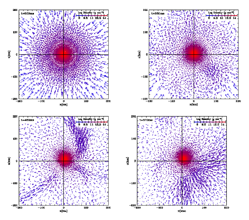
Figure 5: 4 snapshots in time of the central region surrounding the neutron star. We plot slices of the data in the x-z plane. The vectors denote direction and magnitude of the particle motion. The proto-neutron star does not move considerably until convection produces downflows that impart “mini-kicks” onto the proto-neutron star.

Figure 5 shows 4 snapshots in time of the central 200 km of our calculation. The proto-neutron star has moved slightly before the onset of convection due to slight asymmetries in the collapse conditions. But the real motion occurs after convection becomes strong and downflows “kick” the neutron star. The net kick arises as convective downflows flow down and strike the proto-neutron star, giving it a series of “mini-kicks”. Calculations using the same code used here, but with a 15 instead of 23 M_⊙ star, higher resolution, and the Herant et al. (1994) coupled equation of state did not exhibit this motion without using large seeds in the collapsing core (see discussion in Fryer 2004). This is almost certainly caused by the delay in the explosion, as was suggested by Scheck et al. (2004). Note that the gravity solver in SNSPH is ideally suited for motion of the neutron star and has been shown to behave well in such difficult gravitational calculations (Fryer et al. 2006a), so we believe these motions are real (with the caveat that the small perturbations in the initial model, although representative of what we expect of collapse progenitors, is artificially placed in our initial conditions).

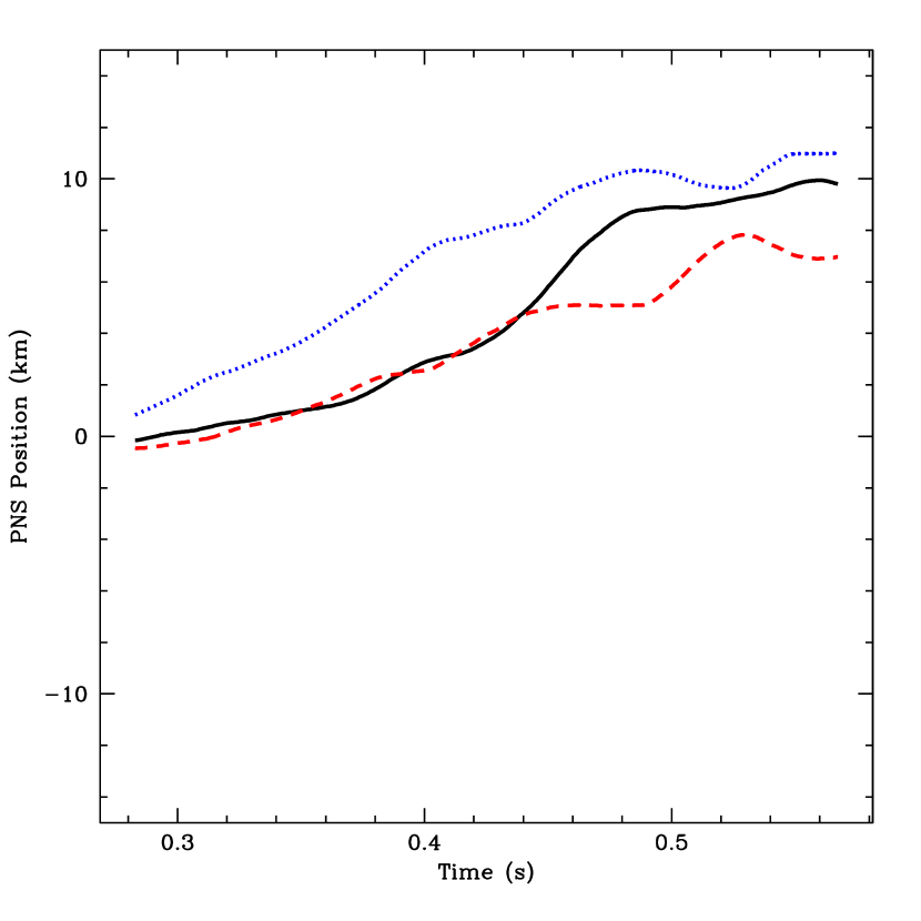
Figure 6: The x (solid), y (dotted), and z (dashed) center of mass positions of the proto-neutron star as a function of time. We have defined material in the proto-neutron star as that material whose density exceeds $10^{13}{\rm gcm^{-3}}$. The motion is not monotonic, but driven by the downflows that buffeting the proto-neutron star. However, there is a systematic trend in the motion of the neutron star, initially seeded by a slight density perturbation in the collapsing star.

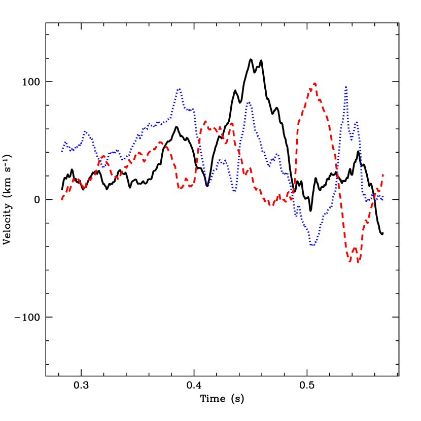
Figure 7: The x (solid), y (dotted), and z (dashed) velocities of the proto-neutron star as a function of time. We have defined material in the proto-neutron star as that material whose density exceeds $10^{13}{\rm gcm^{-3}}$. The velocities are definitely erratic caused by the kicks imparted by downflows onto the proto-neutron star. Because no low-order mode develops and the downflows do not impart cumulative kicks. In this calculation the proto-neutron star velocity never exceeds $\sim 150{\rm kms^{-1}}$, but the velocity is comparable to the low-velocity subset of the Scheck et al. (2004) calculations. Note that we don’t see any rapid oscillations of a ringing neutron star.

The x,y,z position of the proto-neutron star center-of-mass is shown in Fig. 6. Here we have defined the proto-neutron star as all matter with densities in excess of $10^{13}\,{\rm\,g\,cm^{-3}}$. The motion of the neutron star is not monotonic, but there is a basic trend in its motion. In Fig. 7, the velocity components of this neutron star clearly show why such oscillations in the positions occur. The proto-neutron star velocities oscillate with amplitudes above 100 km s^-1, but these large amplitudes occur over 100 ms time periods. The power in these oscillations is less than $5\times 10^{48}{\rm erg\,s^{-1}}$, much lower than that predicted by Burrows et al. (2006). The velocity oscillations are caused by the time evolution of the downflows and the location at which they strike the proto-neutron star.

A pressure wave could move through the star without significantly moving any of the matter. To test if the pressure in a shell of matter is varying widely with time, we plot the time evolution of 9 particles 35 km from the center of the neutron star (Fig 8). The time resolution in this plot is roughly 0.04 ms. At the 0.04 ms timescale, we do not see large oscillations in the pressure of the particles. The particles slowly compress, and there is some variation at timescales comparable to our downflow timescales, but no obvious ringing. We must now try to understand why we do not observe the ringing of the neutron star found in the Burrows et al. (2006) models. It is possible that the smooth particle hydrodynamics technique is damping out any possible pressure perturbations. It is also possible that real damping (e.g. Silk damping) is preventing these oscillations (Ramirez-Ruiz, private communication).

Figure 9 shows the mass of the compact remnant as a function of time. The compact remnant steadily accretes mass during the convective phase as material piles up and cools onto the neutron star. By the time the explosion occurs, the baryonic mass of the remnant exceeds 1.8 M_⊙. Because the explosion is weak ($<10^{51}$ erg), this remnant will accrete further through fallback and will certainly form a black hole. The large mass is a common feature in delayed explosions for progenitors stars more massive the 15 M_⊙. Stars above this mass that have such long delays in their explosion will not produce generic neutron stars. Recall that the long delay is, in part, caused by low resolution in the convection and, in part, by the massive progenitor.

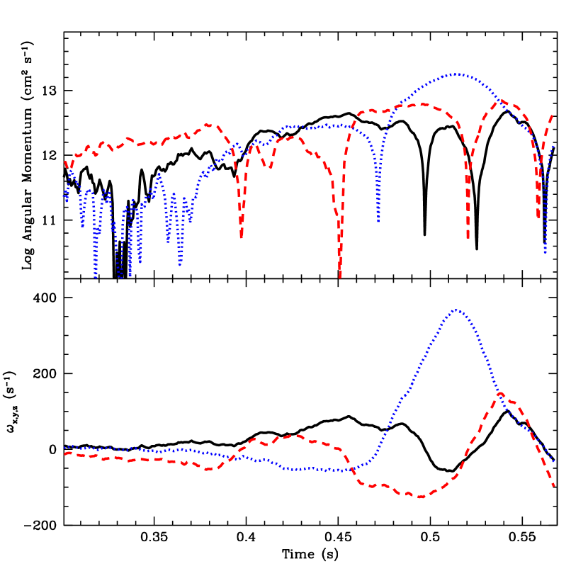
Figure 10: The absolute value of the x (solid), y (dotted) and z (dashed) angular momenta (top) of the neutron star as a function of time. The spikes correspond to a change in sign of the angular momentum. The bottom panel shows the corresponding x (solid), y (dotted) and z (dashed) angular velocity as a function of time. The corresponding period is $2\pi/|\omega|$. The neutron star achieves periods that are as fast as 16 ms, but at the end of the simulation, the period is closer to 1 s.

The downflows also carry a modest amount of angular momentum down into the neutron star. The top panel in figure 10 shows the absolute value of the x,y, and z components of the specific angular momentum in the proto-neutron star as a function of time. The bottom panel shows the x,y, and z components of the angular velocity. Note that the direction of the spin changes as a function of time, but the spin never reaches periods below 15 ms and 1 s spin periods are more typical. But it is possible that spin periods in the tens of milliseconds can be achieved even if the progenitor itself is not rotating.

During the convection, the neutron star is, at times, moving rapidly and, at times, spinning rapidly. But how are these two related. Figure 11 shows the relationship between the kick velocity and the neutron star spin. The top panel shows the angle between the velocity and spin vectors ($\mathbf{v}\cdot\mathbf{\omega}/|\mathbf{v}|/|\mathbf{\omega}|$) as a function of neutron star velocity at all points in time. The bottom panel shows the magnitude of the spin versus the neutron star velocity. Depending upon when the explosion occurs, we can obtain a range of results. One might expect, since it is the accretion of the downflows that both produces the kick and the spin, the two values might evolve together. However, with this single model, it does not appear that there is any correlation between velocity and spin, nor of the direction of the spin with respect to the velocity. More simulations are required to determine whether this lack of correlation is a property of this explosion mechanism.

5 Implications

5.1 On Supernovae

In the collapse of a 23 M_⊙ star with our SNSPH code using low resolution, we obtain an extremely weak explosion at late times (400 ms after bounce). In this delayed explosion, we see effects from both Rayleigh Taylor and spherical accretion shock instabilities. We do not produce a dominant $l=1$ mode in our convection, but it is present at late times just prior to the explosion. The convective downflows “kick” the proto-neutron star, giving it velocities as high as 150 km s^-1. This is comparable to the low velocity set of simulations by Scheck et al (2004). Although our neutron star does not receive a large ($>450$ km s^-1) kick, we can not rule out such large kicks with mildly different initial conditions. Indeed, it is likely that different conditions (both in the initial star and the numerical setup) could produce larger kicks (e.g. Fryer 2004; Scheck et al. 2004).

Our proto-neutron star is definitely buffeted by the downflows. And although these downflows do impart a kick onto the neutron star, we do not see any ringing or oscillations in the proto-neutron star. This result does not agree with the recent work of Burrows et al. (2006). A number of reasons could cause this difference. Numerical viscosity in the particles making up the proto-neutron star could be damping out these oscillations. But the difference may be due to the fact that our simulation did not exhibit the dominant $l=1$ mode convective cycle seen by Burrows et al. (2006). It may be that this dominant mode is necessary to drive oscillations. Fortunately, such questions can be studied using perturbation analysis coupled with a detailed understanding of the equation of state (Arras et al. 2006). In any event, both our convective engine and that of Burrows et al. (2006) takes far too long for this progenitor to make a normal neutron star. It is likely that both explosion mechanisms will produce black holes.

Because the explosion takes so long to occur, the neutron star cools with a heavy mantle of material on top of it. This mantle ultimately places all the neutrinosphere (radius of last scattering) for the electron neutrino and electron anti-neutrinos at roughly the same position. Hence, the energies of these two neutrino species are nearly identical. Figure 12 shows the evolution of the neutrino energies and luminosities for the 3 species followed in this calculation: electron neutrino ($\nu_{e}$), electron anti-neutrino ($\bar{\nu}_{e}$), and all others ($\nu_{x}\equiv$ $\mu,\tau$ neutrinos and anti-neutrinos). The electron neutrino energy is under 12 MeV whereas the electron anti-neutrino energy is under 14 MeV. Such small differences between the neutrino energies is consistent with many of the other delayed supernova explosions (e.g. Buras et al. 2006). Note that the flux-limited diffusion calculation tends to overestimate the mean neutrino energy by $\sim$10% (Budge et al. 2006). The $\sim$ factor of 2 higher flux coming out in electron neutrinos (with energies that are only $<$20% lower) means that matter above the neutrinosphere will preferentially absorb electron neutrinos, leading to an increase in its electron fraction. This will play a role in the nucleosynthetic yields (studied in a later paper) from this explosion.

Neutron star spins at the tens of milliseconds level are possible even with a non-rotating progenitor. For spin-periods below 10 ms, it is likely that a rotating progenitor is required.

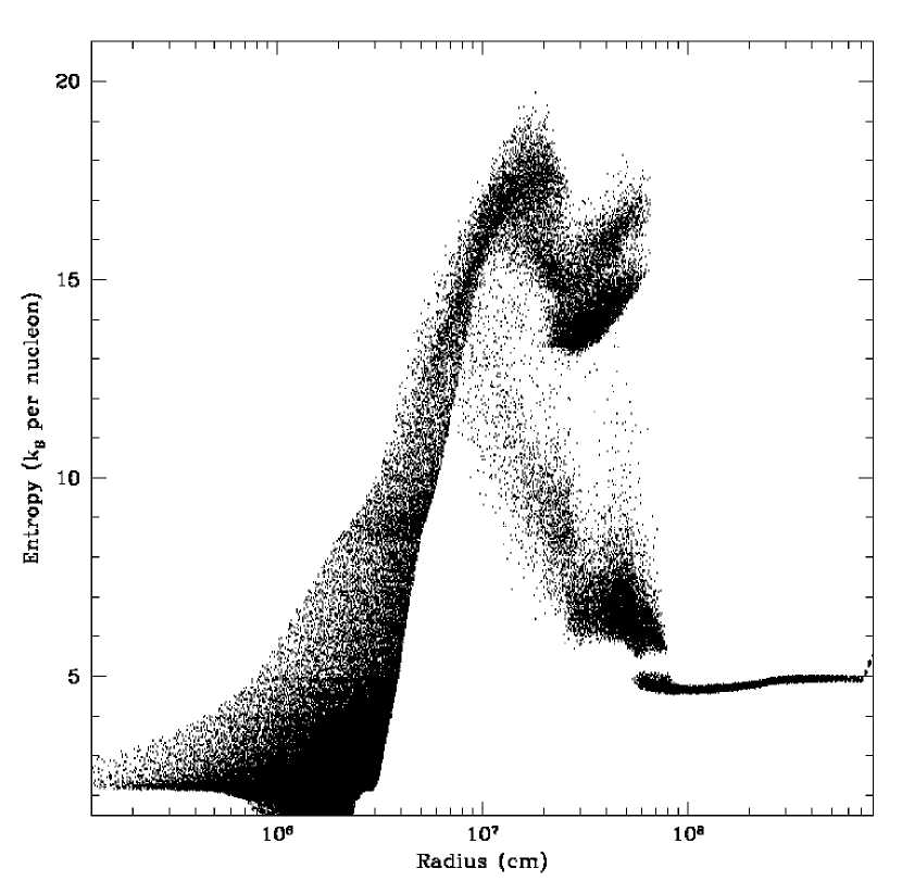
Figure 13: Entropy (in units of Boltzmann constant per nucleon) as a function of radius for our stellar core 600 ms after collapse. Even at these late times, the peak entropy is less than 20 $k_{\rm B}$ per nucleon. The downflows are characterized by the low entropy material.

The entropy profile of our star 600 ms after collapse is shown in figure 13. Even at these late times, the peak entropies do not rise above 20 $k_{\rm B}$ per nucleon. Such low entropies would not be high enough to produce the r-process in a wind-driven trajectory. But the trajectories in this convective region are very different from the wind-driven trajectories, and the trajectory can be more important in determining the actual yield of a piece of matter than the entropy or electron fraction in that matter (see, for example, Meyer 2002 or Fryer et al. 2006d). We defer discussion of the exact yields of this collapse to a later paper.

It has been over a decade since the first collapse and explosion calculations in 2-dimensions suggested that convection play a crucial role in the core-collapse supernova engine. We now know several different convective instabilities (even without including the effects of magnetic fields). To truly understand the role these instabilities play in supernovae, we will have to understand the limitations of our numerical techniques. Without much higher resolution, or new techniques for including artificial viscosity, our SNSPH code is limited to low Reynolds number flows. Most grid codes suffer from similar viscosities and peculiarities due to advection terms. Techniques for solving gravity and estimates for the equation of state also can alter the convection. If convection is an important ingredient of the supernova engine, we have our work cut out for us.

5.2 On Hypernovae and Black Holes

Fryer (1999) argued that 23 M_⊙ stars lie at the transition between neutron star and black hole formation. As such, these stars are subject to a range of outcomes. The delay in the explosion allows time for large magnetic fields to develop and it is possible that if this star were rotating, large magnetic fields would develop that could dominate the explosion. In addition, as the proto-neutron star’s mass increases, it is possible that a transition to quark matter can occur, producing an explosion. Lastly, if the star collapses to a black hole, it can produce an explosion via a black hole accretion disk engine (Popham et al. 1999). The fact that we are in this transition region means that a wide range of explosive fates exist for these stars.

Without magnetic fields or a transition to a quark star injecting energy, this star will ultimately accrete so much material that it will collapse to form a black hole. If the star were rotating, it would be a candidate star for the production of a hypernova (and even the subclass of hypernovae that produce gamma-ray bursts). These calculations have some important implications for the hypernova engine. In this simulation, the collapse initially produces a massive neutron star that, through fallback, collapses to form a black hole. In such a scenario, we will get a weak supernova explosion followed within a few seconds of a collapse to a black hole and a hypernova jet explosion. Depending upon this delay, the ⁵⁶Ni produced can vary dramatically (Fryer et al. 2006b). This delay also allows the massive newly-formed neutron star to move away from the “center” of the star. Recall that we found kicks as high as $150\,{\rm km\,s^{-1}}$ in our calculation (and the Sheck et al. (2004) results very large kicks $1000\,{\rm km\,s^{-1}}$ are possible). If the hypernova engine does not turn on until a few seconds after collapse, the black hole may well be over 1000 km away from the star’s center when it turns on.

Even if the explosion does not occur and the the core collapses directly to a black hole, we must still pass through a phase of long-term convection. This convection will very likely develop low mode convection (this depends upon how far the convective region moves outward) and the compact remnant will be kicked. In the most conservative case where there is no matter carrying out momentum, asymmetric neutrino emission will carry out momentum to produce a kick on the black hole, and it is likely that all (even direct-collapse) black holes are born with moderate kicks. Past estimates (e.g. Fryer ) have suggested that black holes receive kicks with comparable momenta to the neutron star velocity distribution ($v_{\rm BH}/v_{\rm NS}=M_{\rm NS}/M_{\rm BH}$). What we expect from these models (and assuming this asymmetric convection is the source of kicks on compact remnants) is instead that the black hole velocity distribution is comparable to the neutron star distribution. The affect of this kick distribution on black hole binary systems remains to be seen.

Figure 2: Density (top) and Temperature (bottom) as a function of enclosed mass for our progenitor (solid line: Young et al. 2006), a KEPLER progenitor (dotted line: Heger et al. 2006), and the standard s15s7b2 model (dashed line: Woosley & Weaver 1995). Note the jumps in density just above 2.1 M_⊙ and 2.7 M_⊙. This occurs because of the sharp transition between shells in the KEPLER code. It does not occur in our progenitor. Our progenitor also has higher densities beyond about 1.5 M_⊙.

Figure 3: Accretion rate as a function of enclosed mass (top) and time (bottom) for 3 progenitors: our progenitor (solid line: Young et al. 2006), a KEPLER progenitor (dotted line: Heger et al. 2006), and the standard s15s7b2 model (dashed line: Woosley & Weaver 1995). This accretion rate is a good simple (but not complete) indicator of the fate of the star where stars with higher mass accretion rates are harder to explode. Note that at 0.65 s (roughly 0.4 s after bounce), the difference between the KEPLER model and our progenitor (both 23 M_⊙ stars) is roughly equal to the difference between the KEPLER model and model s15s7b2. Clearly, the uncertainty in stellar progenitor codes is still large.

Figure 8: Pressure versus time for 9 particles lying 35 km from the center of the neutron star. This plot has 400 time dumps corresponding to 0.04 ms time resolution. The primary evolution of the pressure is a steady increase as matter continues to pile onto the neutron star. Some variation exists on ms timescales, but at the 1% level, corresponding to energy injection below $10^{44}{\rm\,erg\,s^{-1}}$.

Figure 9: Mass of the neutron star as a function of time. Because of the long delay in this explosion, the mass of the neutron star has grown beyond 1.8 M_⊙ prior to the launch of the explosion. Clearly such a long delay will not make a “typical” neutron star. Indeed, with the weak explosion energies from this explosion, we expect to have considerable fallback and the final remnant of this object will be a black hole. This points out a difficulty with models requiring long delays - for stars above $\sim 15\,$M_⊙, such long delays produce massive neutron stars or black holes.

Figure 11: The angle between neutron star velocity and spin vectors (top) and magnitude of the spin velocity (bottom) as a function of the magnitude of the velocity at different times in the explosion. Although both the velocity and spin rate evolve through accretion, there is no correlation between the spin and the velocity.

Figure 12: Neutrino energy (top) and neutrino luminosity (bottom) as a function of time for the 3 species followed in the simulation: electron neutrino (solid), electron anti-neutrino (dotted), $\mu$ and $\tau$ neutrinos (dashed). Note that the electron anti-neutrino energies are $<20\%$ higher than the electron neutrino energies at the end of the simulation, but their fluxes are a factor of 2 lower.

References

- Balsara (1995) Balsara, D.S. 1995, Journ. of Comp. Phys., 121, 357
- Bazan & Arnett (1998) Bazan, G., & Arnett, D. 1998, ApJ, 496, 316
- Blondin et al. (2003) Blondin, J.M., Mezzacappa, A., & DeMarino, C. 2003, ApJ, 584, 971
- Blondin & Mezzacappa (2006) Blondin, J.M., & Mezzacappa, A. 2006, ApJ, 642, 401
- Braginskii (1958) Braginskii, S.I. 1958, JETP, 6, 358
- Budge et al. (2006) Budge, K. et al. in preparation
- Buras et al. (2003) Buras, R., Rampp, M., Janka, H.-Th., Kifonidis, K. 2003, PRL, 90, 1101
- Buras et al. (2006) Buras, R., Rampp, M., Janka, H.-Th., Kifonidis, K. 2006, A&A, 447, 1049
- Burrows et al. (1995) Burrows, A., Hayes, J., & Fryxell, B.A. 1995, ApJ, 450, 830
- Burrows et al. (2006) Burrows, A., Livne, E., Dessart, L., Ott, C.D., & Murphy, J. 2006, ApJ, 640, 878
- Bruenn et al. (2004) Bruenn, S.W., Raley, E.A., & Mezzacappa, A. 2004, submitted to ApJ, astro-ph 0404099
- Cox et al. (1983) Cox, A.N., Vauclair, S., & Zahn, J.P. 1983, Astrophysical Processes in Upper Main Sequence Stars (CH-1290 Sauverny: Geneva Observatory)
- Epstein (1979) Epstein, R.I. 1979, MNRAS, 188, 305
- Foglizzo et al. (2005) Foglizzo, T., Galleti, P., & Ruffert, M. 2005, A&A, 435, 397
- Foglizzo et al. (2006) Foglizzo, T., Galleti, P., Scheck, L., & Janka, H.-Th. 2006, astro-ph/0606640
- Fryer et al. (1996) Fryer, C.L., Benz, W., & Herant, M. 1996, ApJ, 460, 801
- Fryer et al. (1998) Fryer, C.L., Burrows, A., & Benz, W. 1998, ApJ, 496, 333
- Fryer (1999) Fryer, C.L. 1999, ApJ, 522, 413
- Fryer & Warren (2002) Fryer, C.L. & Warren, M.S. 2002, ApJ, 574, L65
- Fryer (2003) Fryer, C.L., IJMPD, 12, 1795
- Fryer (2004) Fryer, C.L. 2004, ApJ, 601, L175
- Fryer & Warren (2004) Fryer, C.L. & Warren, M.S. 2004, ApJ, 601, 391
- Fryer & Kusenko (2006) Fryer, C.L., & Kusenko, A. 2006, ApJS, 163, 335
- Fryer et al. (2006a) Fryer, C.L., Rockefeller, G., & Warren, M.S. 2006, ApJ, 643, 292
- Fryer et al. (2006b) Fryer, C.L., Young, P.A., & Hungerford, A.L. 2006, accepted by ApJ
- Fryer et al. (2006c) Fryer, C.L., Hungerford, A.L., & Rockefeller, G., 2006, IJMPD, in preparation
- Fryer et al. (2006d) Fryer, C.L., Herwig, F., Hungerford, A.L., & Timmes, F.X., 2006, submitted to ApJ
- Heger et al. (2006) Heger, A. et al. 2006, in preparation
- Herant et al. (1994) Herant, M., Benz, W., Hix, W.R., Fryer, C.L., & Colgate, S.A. 1994, ApJ, 435, 339
- Herant (1995) Herant, M. 1995, Phys. Rep. 256, 117
- Hix & Thielemann (1996) Hix, W.R., & Thielemann, F.-K. 1996, ApJ, 460, 869
- Houck & Chevalier (1991) Houck, J.C., & Chevalier, R.A. 1991, ApJ, 376, 234
- Houck & Chevalier (1992) Houck, J.C., & Chevalier, R.A. 1992, ApJ, 395, 592
- Janka et al. (2005) Janka, H.-T., Buras, R., Kitaura Joyanes, F.S., Marek, A., Rampp, M., Scheck, L. 2005, Nuc. Phys. A, 758, 19
- Keil et al. (1996) Keil, W., Janka, H.-T., Müller, E. 1996, ApJ, 473, L111
- Lai et al. (2001) Lai, D., Chernoff, D.F., & Cordes, J.M. 2001, ApJ, 549, 1111
- Lattimer & Swesty (1991) Lattimer, J.M. & Swesty, F.D. 1991, Nucl. Phys. A, 535, 331
- (38) Meakin, C.A., & Arnett, D. 2006, ApJ, 637, L53
- (39) Meakin, C.A., & Arnett, D. 2006, ApJ, submitted
- Meakin, Young, & Arnett (2005) Meakin, Casey, Young, Patrick A., & Arnett, David 2005, ApJ, submitted
- Mezzacappa et al. (1998) Mezzacappa, A., Calder, A.C., Bruenn, S.W., Blondin, J.M., Guidry, M.W., Strayer, M.R., & Umar, A.S. 1998, ApJ, 493, 848
- Meyer (2002) Meyer, B.S. 2002, PRL, 89, 1101
- Ohnishi et al. (2006) Ohnishi, N., Kotake, K., Yamada, S. 2006, ApJ, 641, 1018
- Popham et al. (1999) Popham, R., Woosley, S.E., & Fryer, C.L. 1999, ApJ, 518, 356
- Scheck et al. (2004) Scheck, L., Plewa, T., Janka, H.-Th., Kifonidis, K., Müller, E. 2004, PRL, 92, 1103
- Schmidt et al. (2006) Schmidt, W., Hillebrandt, W., & Niemeyer, J.C. 2005, Comp. Fluids., 35, 353
- Simon (1949) Simon, A. 1949, Phys. Rev., 100, 75, 1912
- Spitzer (1962) Spitzer, L. 1962, Physics of Fully Ionized Gases (Physics of Fully Ionized Gases, New York: Interscience (2nd edition), 1962)
- Woosley & Weaver (1995) Woosley, S.E., & Weaver, T.A. 1995, ApJS, 101, 181
- Yamasaki & Yamada (2006) Yamasaki, T. & Yamada, S. 2006, ApJ, 650, 291
- Young & Arnett (2005) Young, P. A. & Arnett, D. 2005, ApJ, 618, 908
- Young et al. (2005) Young, P. A., Meakin, C., Arnett, D., & Fryer, C.L. 2005, ApJ, 629, L101
- Young & Fryer (2006) Young, P.A., & Fryer, C.L. 2006, in preparation