Magnetic Hydrogen Atmosphere Models and the Neutron Star RX J1856.5$-$3754

Abstract

RX J1856.5$-$3754 is one of the brightest nearby isolated neutron stars, and considerable observational resources have been devoted to it. However, current models are unable to satisfactorily explain the data. We show that our latest models of a thin, magnetic, partially ionized hydrogen atmosphere on top of a condensed surface can fit the entire spectrum, from X-rays to optical, of RX J1856.5$-$3754, within the uncertainties. In our simplest model, the best-fit parameters are an interstellar column density $N_{\rm H}\approx 1\times 10^{20}\mbox{cm${}^{-2}$}$ and an emitting area with $R^{\infty}\approx 17$ km (assuming a distance to RX J1856.5$-$3754 of 140 pc), temperature $T^{\infty}\approx 4.3\times 10^{5}$ K, gravitational redshift $z_{g}\sim 0.22$, atmospheric hydrogen column $y_{\rm H}\approx 1\mbox{ g cm${}^{-2}$}$, and magnetic field $B\approx(3-4)\times 10^{12}$ G; the values for the temperature and magnetic field indicate an effective average over the surface. We also calculate a more realistic model, which accounts for magnetic field and temperature variations over the neutron star surface as well as general relativistic effects, to determine pulsations; we find there exist viewing geometries that produce pulsations near the currently observed limits. The origin of the thin atmospheres required to fit the data is an important question, and we briefly discuss mechanisms for producing these atmospheres. Our model thus represents the most self-consistent picture to date for explaining all the observations of RX J1856.5$-$3754.

1 Introduction

Seven candidate isolated, cooling neutron stars (INSs) have been identified by the ROSAT All-Sky Survey, of which the two brightest are RX J1856.5$-$3754 and RX J0720.4$-$3125 (see Treves et al. 2000; Pavlov, Zavlin, & Sanwal 2002; Kaspi, Roberts, & Harding 2006 for a review). These objects share the following properties: (1) high X-ray to optical flux ratios of $\log(f_{\rm X}/f_{\rm optical})\sim 4-5.5$, (2) soft X-ray spectra that are well described by blackbodies with $kT\sim 50-100$ eV, (3) relatively steady X-ray flux over long timescales, and (4) lack of radio pulsations.

For the particular INS RX J1856.5$-$3754, single temperature blackbody fits to the X-ray spectra underpredict the optical flux by a factor of $\sim 6-7$ (see Fig. 8). X-ray and optical/UV data can best be fit by two-temperature blackbody models with $kT^{\infty}_{\rm X}=63$ eV, emission size $R^{\infty}_{\rm X}=5.1\,(d/\mbox{140 pc})$ km, $kT^{\infty}_{\rm opt}=26$ eV, and $R^{\infty}_{\rm opt}=21.2\,(d/\mbox{140 pc})$ km (Burwitz et al. 2001, 2003; van Kerkwijk & Kulkarni 2001a; Braje & Romani 2002; Drake et al. 2002; Pons et al. 2002; see also Pavlov et al. 2002; Trümper et al. 2004), where $T^{\infty}=T_{\rm eff}/(1+z_{g})$, $R^{\infty}=R^{\rm em}(1+z_{g})$, and $R^{\rm em}$ is the physical size of the emission region. The gravitational redshift $z_{g}$ is given by $(1+z_{g})=(1-2GM/Rc^{2})^{-1/2}$, where $M$ and $R$ are the mass and radius of the NS, respectively. However, the lack of X-ray pulsations (down to the 1.3% level) puts severe constraints on such two-temperature models (Drake et al. 2002; Ransom, Gaensler, & Slane 2002; Burwitz et al. 2003). It is possible that the magnetic axis is aligned with the spin axis or the hot magnetic pole does not cross our line of sight (Braje & Romani 2002). Alternatively, RX J1856.5$-$3754 may possess a superstrong magnetic field ($B\ga 10^{14}$ G) and has spun down to a period $>10^{4}$ s (Mori & Ruderman 2003), though Toropina, Romanova, & Lovelace (2006) argue that this last case cannot explain the H$\alpha$ nebula found around RX J1856.5$-$3754 (van Kerkwijk & Kulkarni 2001b). On the other hand, a single uniform temperature is possible if the field is not dipolar but small-scale (perhaps due to turbulence at the birth of the NS; see, e.g., Bonanno, Urpin, & Belvedere 2005, and references therein).

Even though blackbody spectra fit the data, one expects NSs to possess atmospheres of either heavy elements (due to debris from the progenitor) or light elements (due to gravitational settling or accretion); we note that a magnetized hydrogen atmosphere may provide a consistent explanation for the broad spectral feature seen in the atmosphere of RX J0720.4$-$3125 (Haberl et al. 2004; Kaplan & van Kerkwijk 2005). The lack of any significant spectral features in the X-ray spectrum argues against a heavy element atmosphere (Burwitz et al. 2001, 2003), whereas single temperature hydrogen atmosphere fits overpredict the optical flux by a factor of $\sim 100$ (Pavlov et al. 1996; Pons et al. 2002; Burwitz et al. 2003). However, these hydrogen atmosphere results are derived using non-magnetic atmosphere models. Only a few magnetic (fully ionized) hydrogen or iron atmospheres have been considered (e.g., Burwitz et al. 2001, 2003), and even these models are not adequate. Since $kT\sim\mbox{tens of}$ eV for RX J1856.5$-$3754 and the ionization energy of hydrogen at $B=10^{12}$ G is 160 eV, the presence of neutral atoms must be accounted for in the magnetic hydrogen atmosphere models; the opacities are sufficiently different from the fully ionized opacities that they can change the atmosphere structure and continuum flux (Ho et al. 2003; Potekhin et al. 2004), which can affect fitting of the observed spectra.

Another complication in fitting the observational data of RX J1856.5$-$3754 (and RX J0720.4$-$3125) with hydrogen atmosphere models is that the model spectra are harder at high X-ray energies. On the other hand, observations of RX J0720.4$-$3125 suggest it possesses a dipole magnetic field $B\approx 2\times 10^{13}$ G (Kaplan & van Kerkwijk 2005). It is probable then that RX J0720.4$-$3125 (and possibly RX J1856.5$-$3754) is strongly magnetized with $B\sim 10^{13}-10^{14}$ G, and its high energy emission is softened by the effect of vacuum polarization, which can show steeper high energy tails (Ho & Lai 2003). Rather than resorting to a superstrong magnetic field, an alternate possibility is that there exists a “suppression” of the high energy emission. One such mechanism is examined in Motch, Zavlin, & Haberl (2003; see also Zane, Turolla, & Drake 2004), specifically, a geometrically thin hydrogen atmosphere at the surface that is optically thick to low energy photons and optically thin to high energy photons. The high energy photons that emerge then bear the signature of the lower temperature (compared to atmospheres that are optically thick at all energies) at the inner boundary layer (usually taken to be a blackbody) of the atmosphere model; this leads to a softer high energy tail. Motch et al. (2003) find a good fit to RX J0720.4$-$3125 in this case by using a non-magnetic atmosphere model with $kT_{\rm eff}=57$ eV, a hydrogen column density $y_{\rm H}=0.16\mbox{ g cm${}^{-2}$}$, and distance of 204 pc, and assuming a $M=1.4M_{\odot}$, $R=10$ km NS.

We examine this last possibility by fitting the entire spectrum of RX J1856.5$-$3754 with the latest partially ionized hydrogen atmosphere models (constructed using the opacity and equation of state tables from Potekhin & Chabrier 2003) and condensed matter in strong magnetic fields (see van Adelsberg et al. 2005). The goal of the paper is to provide a self-consistent picture of RX J1856.5$-$3754 that resolves the major observational and theoretical inconsistencies: (1) blackbodies fit the spectrum much better than realistic atmosphere models, (2) strong upper limits on X-ray pulsations suggest RX J1856.5$-$3754 may have a largely uniform temperature (and hence magnetic field) over the entire NS surface, (3) the inferred emission size from blackbody fits are either much smaller or much larger than the canonical NS radius of $10-12$ km. Because of observational uncertainties (see Section 3) and the computationally tedious task of constructing a complete grid of models, we do not attempt to prove the uniqueness of our results; rather we try only to reproduce the overall spectral energy distribution and argue for the plausibility of our model.

An outline of the paper is as follows. In Section 2, we describe the atmosphere model (a thin, magnetized atmosphere of partially ionized hydrogen with a condensed surface) and possible ways of producing this atmosphere. A brief description of the observations is given in Section 3. The model fits to the observational data are shown in Section 4. Possible mechanisms for the creation of thin hydrogen atmospheres and pulsations implied by our model are given in Section 5. We summarize and discuss our results in Section 6.

2 Models of Neutron Star Atmospheres

Thermal radiation from a NS is mediated by the atmosphere (with scaleheight $\sim 1$ cm). In the presence of magnetic fields typical of INSs ($B\ga 10^{12}$ G), radiation propagates in two polarization modes (see, e.g., Mészáros 1992). Therefore, to determine the emission properties of a magnetic atmosphere, the radiative transfer equations for the two coupled photon polarization modes are solved. The self-consistency of the atmosphere model is determined by requiring the fractional temperature corrections $\Delta T(\tau)/T(\tau)\ll 1\%$ at each Thomson depth $\tau$, deviations from radiative equilibrium $\ll 1\%$, and deviations from constant flux $<1\%$ (see Ho & Lai 2001; Ho et al. 2003; Potekhin et al. 2004, and references therein for details on the construction of the atmosphere models). We note that the atmosphere models formally have a dependence, through hydrostatic balance, on the surface gravity $g$ $[=(1+z_{g})GM/R^{2}]$ and thus the NS radius $R$; however, the emergent spectra do not vary much using different values of $g$ around $2\times 10^{14}$ cm s^-2 (Pavlov et al. 1995). Nevertheless, we construct models using a surface gravity that is consistent with the inferred radius obtained from the spectral fits in Section 4 ($g=1.1\times 10^{14}$ cm s^-2 with $M=1.4M_{\odot}$, $R=14$ km, and $z_{g}=0.2$). Also, though our atmosphere models can have a magnetic field at an arbitrary angle $\Theta_{B}$ relative to the surface normal, the models considered in Sections 2 and 4 have the magnetic field aligned perpendicular to the stellar surface (see Section 5.1 for justification and other cases). We describe other elements of our atmosphere models below.

2.1 Partially Ionized Atmospheres

As discussed in Section 1, previous works that attempted to fit the spectra of RX J1856.5$-$3754 and other INSs with magnetic hydrogen atmosphere models assume the hydrogen is fully ionized. The temperature obtained using these models (or simple blackbodies) are in the range $kT^{\infty}\approx 40-110$ eV. Contrast this with the atomic hydrogen binding energies of 160 eV and 310 eV at $B=10^{12}$ G and $10^{13}$ G, respectively. Therefore the atmospheric plasma must be partially ionized.

Figure 1 illustrates the spectral differences between a fully ionized and a partially ionized hydrogen atmosphere. The atomic fraction is $<10\%$ throughout the atmosphere, where the atomic fraction is the number of H atoms with non-destroyed energy levels divided by the total number of protons (see Potekhin & Chabrier 2003; Ho et al. 2003). Besides the proton cyclotron line at $\lambda_{Bp}=1966(B/10^{12}\mbox{ G})^{-1}(1+z_{g})$ Å, the other features are due to bound-bound and bound-free transitions. In particular, these are the $s=0$ to $s=1$ transition at (redshifted) wavelength $\lambda=170$ Å, the $s=0$ to $s=2$ transition at $\lambda=110$ Å, and the bound-free transition at $\lambda=61$ Å. The quantum number $s$ measures the $B$-projection of the relative proton-to-electron angular momentum (see, e.g., Lai 2001). For a moving atom, this projection is not an integral of motion, but nonetheless the quantum number $s$ (or $m=-s$) remains unambiguous and convenient for numbering discrete states of the atom (see Potekhin 1994). Because of magnetic broadening, the features resemble dips rather than ordinary spectral lines (see Ho et al. 2003).

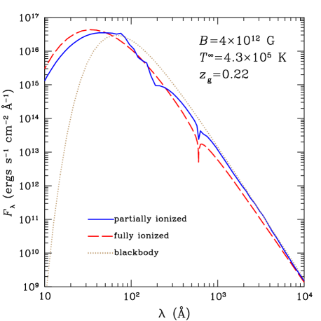
Figure 1: Spectra of hydrogen atmospheres with $B=4\times 10^{12}$ G, and $T^{\infty}=4.3\times 10^{5}$ K. The solid line is for a partially ionized atmosphere, the dashed line is for a fully ionized atmosphere, and the dotted line is for a blackbody. All spectra are redshifted by $z_{g}=0.22$.

2.2 Thin Atmospheres

Conventional NS atmosphere models assume the atmosphere is geometrically thick enough such that it is optically thick at all photon energies ($\tau_{\lambda}\gg 1$ for all wavelengths $\lambda$, where the optical depth is $\tau_{\lambda}=\int\chi_{\lambda}\,ds$, the extinction coefficient is $\chi_{\lambda}$, and the distance traveled by the photon ray is $ds$); thus the observed photons are all created within the atmosphere layer. The input spectrum (usually taken to be a blackbody) at the bottom of the atmosphere is not particularly important in determining the spectrum seen above the atmosphere since photons produced at this innermost layer undergo many absorptions/emissions. The observed spectrum is determined by the temperature profile and opacities of the atmosphere. For example, atmosphere spectra are harder than a blackbody (at the same temperature) at high energies as a result of the non-grey opacities (see Fig. 1); the opacities decline with energy so that high energy photons emerge from deeper, hotter layers in the atmosphere than low energy photons.

On the other hand, consider an atmosphere that is geometrically thinner than described above, such that the atmosphere is optically thin at high energies but is still optically thick at low energies ($\tau_{\lambda}<1$ for $\lambda<\lambda_{\rm thin}$ and $\tau_{\lambda}>1$ for $\lambda>\lambda_{\rm thin}$). Thus photons with wavelength $\lambda<\lambda_{\rm thin}$ pass through the atmosphere without much attenuation (and their contribution to thermal balance is small since most of the energy is emitted at $\lambda>\lambda_{\rm thin}$ in the case of RX J1856.5$-$3754). If the innermost atmosphere layer (at temperature $T_{\rm thin}$) emits as a blackbody, then the observed spectrum at $\lambda<\lambda_{\rm thin}$ will just be a blackbody spectrum at temperature $T=T_{\rm thin}$. Motch et al. (2003) showed that a “thin” atmosphere can yield a softer high energy spectrum than a “thick” atmosphere and used a thin atmosphere spectrum to fit the observations of RX J0720.4$-$3125.

The method for constructing a thin atmosphere does not differ significantly from that used for a thick atmosphere (see Ho & Lai 2001 for details on thick atmosphere construction). The difference is that, instead of computing the model to large Thomson depths (where $\tau_{\lambda}\gg 1$ for all $\lambda$), we go to a relatively shallow depth at density $\rho_{\rm thin}$. At this shallow depth, we adjust the inner boundary condition (depending on the model, either a blackbody or a condensed surface spectrum; see Section 2.3) to account for reflections. The temperature profile is mainly determined by the radiative flux (through radiative equilibrium) and mean opacities. For instance, the profile is nearly the same in the thin and thick atmosphere models shown in Figure 2 because the bulk of the radiative energy comes from wavelengths for which the atmosphere is optically thick; this is clearly seen in Figure 3, which plots the atmosphere spectra seen by a distant observer. Thus, the difference in the spectra at short wavelengths basically does not affect the mean (Rosseland-like) opacities and the resulting temperature profile. The only noticeable deviation occurs near the condensed surface and is due to the boundary condition imposed at this depth. For comparison, Figure 4 shows a profile with still lower $\rho_{\rm thin}$. In this case, the boundary between the optically thick and thin portions of the spectrum lies at a longer wavelength. Since the integrated flux is more sensitive to the spectral difference at these longer wavelengths (being closer to the peak of the spectrum), we see a more noticeable difference in the temperature profiles. A qualitatively similar result is obtained for the same atmosphere thickness but with a higher effective temperature, since the peak flux is shifted to shorter wavelengths.

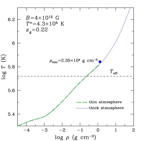
Figure 2: Model atmosphere temperature profiles with $B=4\times 10^{12}$ G and $T^{\infty}=4.3\times 10^{5}$ K. The dotted and long-dashed lines are the “thick” atmosphere and “thin” atmosphere with $y_{\rm H}=1.2\mbox{ g cm${}^{-2}$}$, respectively (see text for details). The short-dashed horizontal line indicates the effective temperature ($T_{\rm eff}=5.3\times 10^{5}$ K) of the atmosphere model.

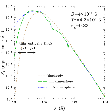
Figure 3: Spectra of hydrogen atmospheres with $B=4\times 10^{12}$ G and $T^{\infty}=4.3\times 10^{5}$ K. The dotted and long-dashed lines are the model spectra using the “thick” atmosphere and “thin” atmosphere with $y_{\rm H}=1.2\mbox{ g cm${}^{-2}$}$, respectively (see text for details). The short-dashed line is for a blackbody with the same temperature. All spectra are redshifted by $z_{g}=0.22$. The vertical line separates the wavelength ranges where the atmosphere is optically thin ($\tau_{\lambda}<1$) and optically thick ($\tau_{\lambda}>1$).

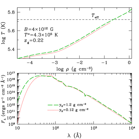
Figure 4: Model atmosphere temperature profiles (top) and spectra (bottom) with $B=4\times 10^{12}$ G and $T^{\infty}=4.3\times 10^{5}$ K. The long-dashed and dotted lines are the “thin” atmospheres with $y_{\rm H}=1.2$ and $0.12\mbox{ g cm${}^{-2}$}$, respectively. The short-dashed horizontal line indicates the effective temperature ($T_{\rm eff}=5.3\times 10^{5}$ K) of the atmosphere model. All spectra are redshifted by $z_{g}=0.22$.

2.3 Condensed Iron Versus Blackbody Emission

In addition to atmosphere models in which the deepest layer of the atmosphere is assumed to be a blackbody, we construct (more realistic and self-consistent) models in which this layer undergoes a transition from a gaseous atmosphere to a condensed surface. A surface composed of iron is a likely end-product of NS formation, and Fe condenses at $\rho\approx 561\,AZ^{-3/5}B_{12}^{6/5}\mbox{ g cm${}^{-3}$}\approx 2.35\times 10^{4}\mbox{ g cm${}^{-3}$}$ and $T\la 10^{5.5}B_{12}^{2/5}\mbox{ K}\approx 5.5\times 10^{5}$ K for the case considered here (Lai 2001); note that there is several tens of percent uncertainty in the condensation temperature (Medin & Lai, private communication; see also Medin & Lai 2006a,b). The hydrogen condensation temperature is also uncertain (see, e.g., Lai & Salpeter 1997; Potekhin, Chabrier, & Shibanov 1999; Lai 2001); the results of Lai (2001) give $T\sim 2\times 10^{4}B_{12}^{0.65}$ K, which suggests much lower temperatures than is relevant for our case. The condensed matter surface possesses different emission properties than a pure blackbody (Brinkmann 1980; Turolla, Zane, & Drake 2004; van Adelsberg et al. 2005; Pérez-Azorín, Miralles, & Pons 2005); in particular, features can appear at the plasma and proton cyclotron frequencies.

We use the calculations of van Adelsberg et al. (2005) to determine the input spectrum in our radiative transfer calculations of the atmosphere. However, at the temperature ($T_{\rm thin}\approx 7\times 10^{5}$ K) of the condensed layer relevant to our thin atmosphere models that fit the spectrum of RX J1856.5$-$3754, the input spectrum (where $\tau_{\lambda}\la 1$) is effectively unchanged from a blackbody (since the temperature profile is nearly identical, with $\Delta T_{\rm thin}\sim 3\%$; see Fig. 2). Thus there are only slight differences in the resulting surface spectrum. This is illustrated in Figure 5, where we show the emission spectrum from a $B=4\times 10^{12}$ G condensed iron surface at $T=7\times 10^{5}$ K and $\rho=2.35\times 10^{4}\mbox{ g cm${}^{-3}$}$ and compare this to a blackbody at the same temperature. The deviation from a blackbody is smaller at low angles (with respect to the magnetic field) of photon propagation $\theta$ and increases for increasing $\theta$, as illustrated by the two angles $\theta=15^{\circ}$ and $60^{\circ}$ (see van Adelsberg et al. 2005). Thus for most angles $\theta$, the condensed surface spectra at short wavelengths (where $\tau_{\lambda}\ll 1$, so that this surface is visible to an observer above the atmosphere) are virtually identical to a blackbody. On the other hand, the atmosphere is optically thick at longer wavelengths, where the condensed surface spectra deviate from a blackbody; thus the condensed surface and the spectral features are not visible. We see from Figure 3 that the harder spectrum at high energies in the “thick” atmosphere becomes much softer in the “thin” atmosphere and takes on a blackbody shape. In contrast, there is a negligible difference where the atmosphere is optically thick.

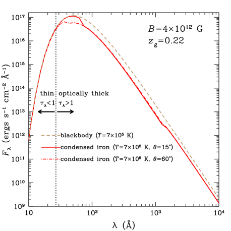
Figure 5: Condensed iron surface spectrum (solid line for photon propagation direction $\theta=15^{\circ}$ and dot-dashed line for $\theta=60^{\circ}$), with $B=4\times 10^{12}$ G, $T=7\times 10^{5}$ K, and $\rho=2.35\times 10^{4}\mbox{ g cm${}^{-3}$}$, compared to a blackbody (dashed line) with the same temperature. All spectra are redshifted by $z_{g}=0.22$. The vertical line separates the wavelength ranges where the atmosphere is optically thin ($\tau_{\lambda}<1$) and optically thick ($\tau_{\lambda}>1$).

3 Observations & Analysis

We collect publically available optical, UV, and X-ray data on RX J1856.5$-$3754. These data have been discussed elsewhere so our treatment will be brief. First, we assemble the optical ($B$- and $R$-band) photometry from the Very Large Telescope (VLT) from van Kerkwijk & Kulkarni (2001a) and the Hubble Space Telescope (HST) WFPC2 F170W, F300W, F450W, and F606W photometry (Walter 2001; Pons et al. 2002) as analyzed by van Kerkwijk & Kulkarni (2001a). We also take the optical VLT spectrum from van Kerkwijk & Kulkarni (2001a) and a STIS far-UV spectrum. The spectra are entirely consistent with the photometry as calibrated by van Kerkwijk & Kulkarni (2001a), although given the limited signal-to-noise ratio of the spectra, we rely primarily on the photometry in what follows. We then use the Extreme Ultraviolet Explorer (EUVE; Haisch, Bowyer, & Malina 1993) data as discussed and reduced by Pons et al. (2002). Finally, we take the RGS spectrum from the 57-ks XMM-Newton observation and the 505-ks Chandra LETG spectrum that are discussed by Burwitz et al. (2003).

A source of uncertainty is that, as mentioned by Burwitz et al. (2003), the RGS and LETG data are not entirely consistent in terms of flux calibration: while they have very similar shapes (and hence implied temperatures and absorptions) the radii inferred from blackbody fits differ by as much as 10% and the overall flux by as much as 20%. Since the LETG fits in Burwitz et al. (2003) are more consistent with those of the CCD instruments on XMM-Newton (EPIC-pn and EPIC-MOS2) and in our opinion the current low-energy calibration of LETG is more reliable, we adjust the flux of the RGS data upward by 17% to force agreement with the Chandra data. We do not know for certain which calibration (if either) is entirely accurate, so some care must be taken when interpreting the results at the 10%–20% level. Fully reliable calibration or even cross-calibration at the low-energy ends of the Chandra and XMM-Newton responses ($<0.2$ keV) is not currently available (see, e.g., Kargaltsev et al. 2005), and the detailed response of EUVE compared to those of Chandra and XMM-Newton is also unknown. Therefore, for accuracy in doing the EUV/X-ray fits, we concentrate on the LETG data, which are consistent and have high-quality calibration.

We follow the HRC-S/LETG analysis threads “Obtain Grating Spectra from LETG/HRC-S Data”, “Creating Higher-order Responses for HRC-S/LETG Spectra”, “Create Grating RMFs for HRC Observations”, and “Compute LETG/HRC-S Grating ARFs” and use CIAO version 3.2.2 and CALDB version 3.2.2. We extracted the dispersed events and generated response files for orders $\pm 1$, $\pm 2$, and $\pm 3$. After fitting the LETG data, we compare the fit results qualitatively with the RGS and EUVE data; the general agreement is good, but we do not use them quantitatively.

4 Atmosphere Model Fitting

Because of data reduction and cross-calibration issues (see Section 3) and possible variations in the interstellar absorption abundances (standard abundances are assumed), we do not feel that a full fit of the data is justified at this time. Therefore we do not fit for all of the parameters in a proper sense nor do we perform a rigorous search of parameter space. Instead, we fit for a limited subset of parameters while varying others manually. This allows us to control the fits in detail and reduce the computational burden of preparing a continuous distribution (in $B$, $T_{\rm eff}$, and $y_{\rm H}$) of models, yet still determine whether our model qualitatively fits the data.

For a given magnetic field and atmosphere thickness, we generate partially ionized atmosphere models for a range of effective temperatures. (Note that, since the continuum opacity of the dominant photon polarization mode decreases for increasing magnetic fields, the required thickness $y_{\rm H}$ of the atmosphere increases for increasing $B$.) We then perform a $\chi^{2}$ fit in CIAO to the LETG data over the 10–100 Å range (0.12–1.2 keV) for the absorption column density $N_{\rm H}$ [using the TBabs absorption model from Xspec (Wilms, Allen, & McCray 2000), although other models such as phabs give similar results], the temperature $T^{\infty}$, the normalization (parameterized by $R^{\infty}$), and the redshift $z_{g}$, where we interpolate over $T^{\infty}$. We obtain a good fit, and Table 1 lists the best-fit parameters and models; the radius is given assuming a distance $d_{140}=d/(140\mbox{ pc})=1$ (see footnote 1). Figure 6 shows the confidence regions for temperature and radius; the covariance between the other fit parameters are not as significant. While we find a range of magnetic fields that give acceptable fits, changes in the magnetic field outside this range (but still within $B=10^{12}-10^{13}$ G) and atmosphere thickness lead to worse fits. At $B>10^{13}$ G, spectral features due to proton cyclotron and bound species appear in the observable soft X-ray range (though they are likely to be broadened; see Section 5.1), which are not seen.

Table 1: Fits to the X-ray Data

	Atmosphere		Blackbody
	Model Parameters
$B$ ($10^{12}$)	3	4
$y_{\rm H}$ (g cm-2)	1.2	1.2
Fit Results
$N_{\rm H}$($10^{20}\mbox{ cm}^{-2}$)	1.18(2)	1.30(2)	0.91(1)
$T^{\infty}$($10^{5}$ K)	4.34(3)	4.34(2)	7.36(1)
$R^{\infty}$($d_{140}$ km)	17	17	5.0
$z_{g}$	0.27(2)	0.22(2)
$\chi_{\rm r}^{2}$/dof	0.85/4268	0.86/4268	0.86/4269

Figure 6: 1, 2, 3$\sigma$ confidence regions for the fit parameters $T^{\infty}$ and $R^{\infty}$ of the $B=4\times 10^{12}$ G atmosphere model. The $3\times 10^{12}$ G model gives very similar results. The dot indicates the best-fit point given in Table 1.

To further evaluate the quality of this fit, we fit the same LETG data with a blackbody. The blackbody fit yields parameters (see Table 1) that are very similar to those derived by Burwitz et al. (2003; see Section 1). A comparison of the residuals for the blackbody fit and the $B=4\times 10^{12}$ G atmosphere model fit is plotted in Figure 7. Given the comparable $\chi_{\rm r}^{2}$ ($\approx 1$) we achieve from our blackbody and atmosphere model fits (along with the low-energy calibration uncertainties), we are confident that the atmosphere model describes the observations just as well as a blackbody.

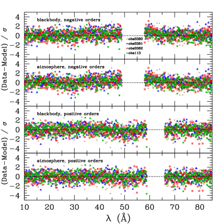
Figure 7: Fit residuals for the blackbody and $B=4\times 10^{12}$ G atmosphere model given in Table 1.

Next, we examine the quality of the fit to the optical/UV data. van Kerkwijk & Kulkarni (2001a) showed that these data are well fit by a Rayleigh-Jeans power law ($F_{\lambda}\propto\lambda^{-4}$) with an extinction $A_{V}=0.12\pm 0.05$ mag. In our fitting, we try using both the optical extinction implied by the X-ray absorption [$A_{V}=N_{\rm H}/(1.79\times 10^{21}\mbox{ cm}^{-2})$ mag; Predehl & Schmitt 1995] and fitting freely for $A_{V}$, but we find that these fits are too unconstrained and that the value of $A_{V}$ is not sensitively determined by the data (indeed, this is reflected in the large uncertainties found by van Kerkwijk & Kulkarni 2001a). As a result, we fix $A_{V}$ to 0.12 mag. We also assume a single value for the reddening ($R_{V}=3.1$) and use the reddening model of Cardelli, Clayton, & Mathis (1989) with corrections from O’Donnell (1994). We find that our best-fit model to the X-ray data also produces a $\lambda^{-4}$ power law but underpredicts the optical/UV data by a factor of 15$-$20%. Looking in detail at the highest quality optical data point (the HST F606W measurement), we find that it is 15% above our model spectra. However, the error budget is 3% (photometric uncertainty), 5% ($A_{V}$ uncertainty), 10% (uncertainty in the optical model flux), and 5% (uncertainty in the fitted optical flux due to the X-ray normalization), and therefore the 15% disagreement can easily be explained by known sources of uncertainty.

Figure 8 shows the observations of RX J1856.5$-$3754. We also overlay the blackbody and our $B=4\times 10^{12}$ G atmosphere model spectra with the parameters given in Table 1. As discussed in Section 1, the data are generally featureless, while the models show spectral features; at $B\approx(3-4)\times 10^{12}$ G, the features due to bound species lie in the extreme UV to very soft X-ray range and are thus hidden by interstellar absorption. Overall, we see that our atmosphere model spectra are generally consistent with the X-ray and optical/UV data, while a blackbody underpredicts the optical/UV by a factor of 6$-$7.

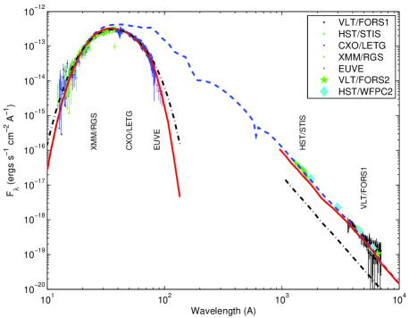
Figure 8: Spectrum of RX J1856.5$-$3754 from optical to X-ray wavelengths. The data points are observations taken from various sources. Error bars are one-sigma uncertainties. Optical spectra are binned for clarity: STIS data into 30 bins at a resolution of 12 Å and VLT data into 60 bins at 55 Å resolution. The solid line is the absorbed (and redshifted by $z_{g}=0.22$) atmosphere model spectrum with $B=4\times 10^{12}$ G, $y_{\rm H}=1.2\mbox{ g cm${}^{-2}$}$, $T^{\infty}=4.3\times 10^{5}$ K, and $R^{\infty}=17$ km. The dashed line is the unabsorbed atmosphere model spectrum. The dash-dotted line is the (absorbed) blackbody fit to the X-ray spectrum with $R^{\infty}=5$ km.

5 Discussion

Two important uncertainties in our model for RX J1856.5$-$3754 are discussed here. The first is flux variability as a result of surface magnetic field and temperature distributions. The second is the creation of thin hydrogen atmospheres.

5.1 Surface Magnetic Field and Temperature Variations and Constraints on Pulsations

A major unexplained aspect of RX J1856.5$-$3754 is the strong observational limit on the lack of pulsations ($\la 1.3\%$). As discussed by Braje & Romani (2002), the low pulsations could be due to an unfavorable viewing geometry and/or a very close alignment between the rotation and magnetic axes. Assuming blackbody emission, they find this is possible in $\sim 5\%$ of viewing geometries (with $R=14$ km). In fact, they note that if RX J1856.5$-$3754 is a normal radio pulsar, then the lack of a radio detection may imply low X-ray pulsations, since the pulsar beam does not cross our line of sight. On the other hand, atmosphere emission can be highly beamed in the presence of a magnetic field (Shibanov et al. 1992; Pavlov et al. 1994) and magnetic field variations over the NS surface will induce surface temperature variations (Greenstein & Hartke 1983). There arises then the questions of whether our single temperature and magnetic field (strength and orientation) atmosphere model fit is physically correct and whether it produces stronger pulsations than is observed. In response to the former, clearly our model spectrum represents an average over the surface and the single temperature and magnetic field indicate “mean” values.

In order to determine the strength of pulsations, synthetic spectra from the whole NS surface must be calculated. Such synthetic spectra are necessarily model-dependent (see, e.g., Zane et al. 2001; Ho & Lai 2004; Zane & Turolla 2005, 2006), as the magnetic field and temperature distributions over the NS surface are unknown. Therefore, we adopt a relatively simple model: we assume the surface is symmetric (in $B$ and $T$) about the magnetic equator and divide the hemisphere into four magnetic latitudinal regions. We generate atmosphere models for each region with the parameters given in Table 2 (note that the magnetic field distribution is roughly dipolar and $\Theta_{B}$ is the angle between the magnetic field and the surface normal). Using an analogous formalism to that described in Pechenick et al. (1983) and Pavlov & Zavlin (2000), we calculate phase-resolved spectra and light curves from the whole NS surface (we assume $M=1.4M_{\odot}$ and $R=14$ km). The resulting phase-resolved spectra have bound and cyclotron features that are broadened due to the surface magnetic field and temperature variations but otherwise are not significantly different from the “local” spectrum we use in Section 4; thus they would produce a qualitatively similar fit. From the light curves, we obtain energy-integrated pulse fractions for the wavelength range 10$-$85 Å (the approximate range of the X-ray observations).

Table 2: Parameters for Neutron Star Surface

magnetic latitude	$B$	$T_{\rm eff}$	$\Theta_{B}$
(deg)	($10^{12}$ G)	($10^{5}$ K)	(deg)
0—10	6	7	0
10—40	5	6	30
40—70	4	5	60
70—90	3	4	90
or
70—90	-	0	-

Assuming the magnetic axis is orthogonal to the rotation axis, $f_{\rm P}<0.01,0.04,0.07$ for $\zeta=10^{\circ},20^{\circ},30^{\circ}$, respectively, where $f_{\rm P}=(F_{\rm max}-F_{\rm min})/(F_{\rm max}+F_{\rm min})$ is the pulse fraction and $\zeta$ is the angle between the rotation axis and the direction to the distant observer. Extending the arguments of Braje & Romani (2002) to realistic atmosphere emission, we thus find there exist viewing geometries for which the pulse fraction is at the observed limits, despite the relatively large magnetic field (and hence strong beaming) and temperature variations. We also note the following: (1) An H$\alpha$ nebula is found around RX J1856.5$-$3754; if interpreted as a bow shock that is powered by the rotational energy loss of a NS magnetic dipole, then the spin period $P\approx 0.5(B/10^{12}\mbox{ G})^{1/2}$ s (van Kerkwijk & Kulkarni 2001b), so that $P\sim 1$ s. (2) The emission can be strongly beamed at higher energies, so that the pulse fraction is energy-dependent; pulsations may be more evident at the higher X-ray energies, although the soft spectrum of RX J1856.5$-$3754 means that broad energy ranges are likely still the most sensitive to pulsations.

5.2 Creation of Thin Hydrogen Atmospheres

From the atmosphere model fits in Section 4 (see also Fig. 3) the critical wavelength $\lambda_{\rm thin}\approx 30$ Å gives an atmosphere column $y_{\rm H}\approx 1-2\mbox{ g cm${}^{-2}$}$. A hydrogen atmosphere with this column density has a total mass of $M_{\rm H}\approx 1\times 10^{13}(R/10\mbox{ km})^{2}(y_{\rm H}/1\mbox{ g cm${}^{-2}$})$ g or about $10^{-21}$ of the mass of a $1.4\,M_{\odot}$ NS. Since the diffusion timescale is extremely short in a high gravity environment (Alcock & Illarionov 1980), the atmosphere contains the bulk of the total hydrogen budget of the NS. The origin of such thin H layers is a problem which we now address by briefly discussing possible mechanisms for generating thin H atmospheres. We leave a more detailed study to future work.

Accretion at low rates may create a thin hydrogen layer on the NS surface. A thin hydrogen layer of $y_{\rm H}=1\,{\rm g\ cm}^{-2}$ has a total mass of $\approx 6\times 10^{-21}\ M_{\odot}$. Hence the time-averaged accretion rate over the age of RX J1856.5$-$3754 ($\sim 5\times 10^{5}$ yr; see Section 6) is $\approx 0.8\,{\rm g\ s}^{-1}$. For the case of RX J0720.4$-$3125 with $y_{\rm H}=0.16\mbox{ g cm${}^{-2}$}$, such a mass layer may result if the time-averaged accretion rate onto the NS is about $0.06\mbox{ g s${}^{-1}$}$ over $10^{6}$ yr. Such small amounts of accretion indicate an enormous fine-tuning problem. Thus this process is unlikely to be the origin of the thin hydrogen envelope.

We next consider the possibility that the thin hydrogen layer is a remnant from the formation of the NS. In this case, Chang & Bildsten (2003, 2004) point out that diffusive nuclear burning (DNB) is the dominant process for determining what happens to hydrogen on the surface of a NS. Due to the power law dependence of the column lifetime $\tau_{\rm col}$ on $y_{\rm H}$, DNB leaves a thin layer of hydrogen, whose thickness depends on the thermal history of the NS and the underlying composition. We find the column lifetime from a full numerical solution to be $\tau_{\rm col}\approx 10^{10}$ yr for a magnetized envelope with $B=10^{12}$ G and $\tau_{\rm col}\approx 10^{8}$ yr for $B=10^{13}$ G (assuming $M=1.4\,M_{\odot}$, $R=14$ km, $T_{\rm eff}=5\times 10^{5}$ K, and $y_{\rm H}=1\mbox{ g cm${}^{-2}$}$). The shorter column lifetime for higher magnetic fields is due to the effect of the magnetic field on the electron equation of state, which increases the hydrogen number density in the burning layer (Chang, Arras, & Bildsten 2004). Thus there is insufficient time at the current effective temperature to reduce the surface hydrogen to such a thin column, assuming that the age of RX J1856.5$-$3754 is $\sim 5\times 10^{5}$ yr. However, DNB was much more effective in the past when the NS was hotter. In fact, during the early cooling history of the NS, DNB would have rapidly consumed all the hydrogen on the surface (Chang & Bildsten 2004). This leads to another fine-tuning problem: if we fix the lifetime of an envelope to some value representing the time the NS spends at a particular temperature, we find that the resulting column scales like $y_{\rm H}\propto T_{\rm eff}^{-40}$ (Chang & Bildsten 2003); therefore, the size of the atmosphere is extremely sensitive to the early cooling history of the NS. As a result, DNB appears to be a less likely mechanism for producing such thin atmospheres.

Finally, we briefly examine a self-regulating mechanism that is driven by magnetospheric currents and may produce thin hydrogen layers on the surface. Since the accelerating potential could be as high as 10 TeV (Arons 1984), high energy particles would create electromagnetic cascades on impact with the surface (Cheng & Ruderman 1977). These cascades result in $e/\gamma$ dissociation of surface material, analogous to proton spallation of CNO elements in accreting systems (Bildsten, Salpeter, & Wasserman 1992). Protons would be one of the products of this dissociation and would rise to the surface due to the rapid diffusion timescale. Since protons cannot further dissociate into stable nuclei, a hydrogen layer is built up to a column roughly given by the radiation length of the ultrarelativistic electrons, beyond which hydrogen can no longer be produced and the above mechanism terminates. The radiation length of ultrarelativistic electrons depends on the stopping physics. In the zero magnetic field limit, the stopping physics is dominated by relativistic bremsstrahlung, and the cross-section is $\sigma\sim\alpha_{\rm F}Z^{2}r_{0}^{2}$, where $\alpha_{\rm F}\equiv e^{2}/\hbar c$ is the fine structure constant, $Z$ is the charge number of the nuclei, and $r_{0}=e^{2}/m_{\rm e}c^{2}$ is the classical electron radius (Bethe & Heitler 1934; Heitler 1954). This gives a stopping column $y_{\rm stop}\sim 3000$ g cm^-2 for hydrogen. Bethe & Ashkin (1953) and Tsai (1974) give a more accurate value, $y_{\rm stop}\sim 60$ g cm^-2, for the stopping column of atomic hydrogen; thus it appears that the resulting columns are too thick. However, for sufficiently strong magnetic fields, the stopping physics of ultrarelativistic electrons is significantly modified, and the dominant stopping mechanism is via magneto-Coulomb interactions (Kotov & Kel’ner 1985; see also Kotov, Kel’ner, & Bogovalov 1986). In magneto-Coulomb stopping, relativistic electrons traveling along field lines are kicked up to excited Landau levels via collisions and de-excite, radiating photons with energy $\gamma\hbar\omega_{B}$, where $\hbar\omega_{B}$ is the Landau cyclotron energy and $\gamma$ is the Lorentz factor of the incoming electron. Compared to zero-field relativistic bremsstrahlung, the magneto-Coulomb radiation length is smaller by a factor of $\sim\pi\alpha_{\rm F}$ (Kotov & Kel’ner 1985). Applying the correction to the Bethe & Ashkin (1953) result ($y_{\rm stop}\sim 60$ g cm^-2), we find this gives roughly the required thin atmosphere column, $y_{\rm stop}\sim 1$ g cm^-2. Though extremely suggestive, this mechanism requires a more complete study and is the subject of future work (see, e.g., Thompson & Beloborodov 2005; Beloborodov & Thompson 2006).

6 Summary and Conclusions

We have gathered together observations of the isolated neutron star RX J1856.5$-$3754 and compared them to our latest magnetic, partially ionized hydrogen atmosphere models. Prior works showed that the observations were well-fit by blackbody spectra. Here we obtain good fits to the overall multiwavelength spectrum of RX J1856.5$-$3754 using the more realistic atmosphere model. In particular, we do not overpredict the optical flux obtained by previous works and require only a single temperature atmosphere. [Note that this single temperature (and magnetic field) serves as an average value for the entire surface.] In addition to the neutron star orientation and viewing geometry, the single temperature helps to explain the non-detection of pulsations thus far. At high X-ray energies, where the atmosphere is optically thin, the model spectrum has a “blackbody-like” shape due to the emission spectrum of a magnetized, condensed surface beneath the atmosphere. The atmosphere is optically thick at lower energies; thus features in the emission spectrum of the condensed surface are not visible when viewed from above the atmosphere. The “thinness” of the atmosphere helps to produce the featureless, blackbody-like spectrum seen in the observations. Using a simple prescription for the temperature and magnetic field distributions over the neutron star surface, we obtain pulsations at the currently observed limits.

Based on a possible origin within the Upper Scorpius OB association, the age of RX J1856.5$-$3754 is estimated to be about $5\times 10^{5}$ yr (Walter 2001; Walter & Lattimer 2002; Kaplan et al. 2002). Our surface temperature determination ($kT^{\infty}=37$ eV) is only a factor of 1.7 below the blackbody temperature ($kT^{\infty}=63$ eV) obtained by previous works (see Sections 1 and 4) and therefore does not place much stronger constraints on theories of neutron star cooling (see, e.g., Page et al. 2004; Yakovlev & Pethick 2004). It may also be noteworthy that RX J1856.5$-$3754 is one of the cooler isolated neutron stars and possibly possesses the lowest magnetic field [$B\approx(3-4)\times 10^{12}$ G]; the lower magnetic field implies a more uniform surface temperature distribution and weaker radiation beaming.

We show that the production of thin hydrogen layers is difficult via accretion or diffusive nuclear burning. Accretion requires a time-averaged rate that is extremely small and fine-tuned. Diffusive nuclear burning has no effect at the current effective temperature but is very efficient when the star was hotter, such that the column thickness depends very sensitively on the early cooling history of the neutron star. Hence these scenarios cannot easily explain the thin atmosphere columns. On the other hand, it may be possible for magnetospheric currents to produce the hydrogen atmospheres if the stopping physics of relativistic electrons is dominated by magneto-Coulomb interactions. We note that younger neutron stars may possess atmospheres composed of helium rather than hydrogen; however, the opacities of bound states of helium in strong magnetic fields is still largely unknown (see, e.g., Al-Hujaj & Schmelcher 2003a,b; Bezchastnov, Pavlov, & Ventura 1998; Pavlov & Bezchastnov 2005).

Finally, the emission radius we derive from our atmosphere model fits is $R^{\infty}\approx 17\,(d/140\mbox{ pc})$ km (although recall the distance and flux uncertainties discussed in footnote 1 and Section 3, respectively). Accounting for gravitational redshift ($z_{g}\sim 0.22$), this yields $R^{\rm em}\approx 14$ km. This is much larger than the inferred radius obtained by just fitting the X-ray data with a blackbody ($R^{\infty}_{\rm X}\approx 5$ km; see Sections 1 and 4). As a result, there does not appear to be a need to resort to more exotic explanations such as quark or strange stars (e.g., Drake et al. 2002; Xu 2003; see Walter 2004; Weber 2005 for a review), at least for the case of RX J1856.5$-$3754. On the other hand, our radius is small compared to the radius derived from fitting the optical/UV data ($R^{\infty}_{\rm opt}\approx 21$ km). For a $1.4\,M_{\odot}$ neutron star, the latter implies a low redshift ($z_{g}\approx 0.12$) and very large intrinsic radius ($R^{\rm em}_{\rm opt}\approx 19$ km); this is ruled out by neutron star equations of state, while our radius $R^{\rm em}\approx 14$ km only requires a standard, stiff equation of state (see, e.g., Lattimer & Prakash 2001).

References

- [Al-Hujaj & Schmelcher(2003a)] Al-Hujaj, O.-A. & Schmelcher, P. 2003a, Phys. Rev. A, 67, 023403
- [Al-Hujaj & Schmelcher(2003b)] Al-Hujaj, O.-A. & Schmelcher, P. 2003b, Phys. Rev. A, 68, 053403
- [Alcock & Illarionov(1980)] Alcock, C. & Illarionov, A. 1980, ApJ, 235, 534
- [Arons (1984)] Arons, J. 1984, Adv. Sp. Res., 3, 287
- [Beloborodov & Thompson(2006)] Beloborodov, A.M. & Thompson, C. 2006, ApJ, in press (astro-ph/0602417)
- [Bethe & Ashkin(1953)] Bethe, H. & Ashkin, J. 1953, in Experimental Nuclear Physics, ed. E. Segrè (New York: Wiley), p.166
- [Bethe & Heitler(1934)] Bethe, H. & Heitler, W. 1934, Proc. Roy. Soc. A, 146, 83
- [Bezchastnov et al.(1998)] Bezchastnov, V.G., Pavlov, G.G., & Ventura, J. 1998, Phys. Rev. A, 58, 180
- [Bildsten et al.(1992)] Bildsten, L., Salpeter, E.E., & Wasserman, I. 1992, ApJ, 384, 143
- [Bonanno et al.(2005)] Bonanno, A., Urpin, V., & Belvedere, G. 2005, A&A, 440, 199
- [Braje & Romani(2002)] Braje, T.M. & Romani, R.W. 2002, ApJ, 580, 1043
- [Brinkmann(1980)] Brinkmann, W. 1980, A&A, 82, 352
- [Burwitz et al.(2003)] Burwitz, V., Haberl, F., Neuhäuser, R., Predehl, P., Trümper, & Zavlin, V.E. 2003, A&A, 399, 1109
- [Burwitz et al.(2001)] Burwitz, V., Zavlin, V.E., Neuhäuser, R., Predehl, P., Trümper, J., & Brinkman, A.C. 2001, A&A, 379, L35
- [Cardelli et al.(1989)] Cardelli, J.A., Clayton, G.C., & Mathis, J.S. 1989, ApJ, 345, 245
- [Chang & Bilsten(2003)] Chang, P. & Bildsten, L. 2003, ApJ, 585, 464
- [Chang & Bilsten(2004)] Chang, P. & Bildsten, L. 2004, ApJ, 605, 830
- [Chang et al.(2004)] Chang, P., Arras, P., & Bildsten, L. 2004, ApJL, 616, L147
- [Cheng & Ruderman (1977)] Cheng, A.F. & Ruderman, M.A. 1977, ApJ, 214, 598
- [Drake et al.(2002)] Drake, J.J., et al. 2002, ApJ, 572, 996
- [Greenstein & Hartke(1983)] Greenstein, G. & Hartke, G.J. 1983, ApJ, 271, 283
- [Haberl et al.(2004)] Haberl, F., Zavlin, V.E., Trümper, J., & Burwitz, V. 2004, A&A, 419, 1077
- [Haisch et al.(1993)] Haisch, B., Bowyer, S., & Malina, R.F. 1993, J. British Interplanetary Society, 46, 331
- [Heitler(1954)] Heitler, W. 1954, Quantum Theory of Radiation, 3rd ed. (London: Oxford University Press)
- [Ho & Lai(2001)] Ho, W.C.G. & Lai, D. 2001, MNRAS, 327, 1081
- [Ho & Lai(2003)] Ho, W.C.G. & Lai, D. 2003, MNRAS, 338, 233
- [Ho & Lai(2004)] Ho, W.C.G. & Lai, D. 2004, ApJ, 607, 420
- [Ho et al.(2003)] Ho, W.C.G., Lai, D., Potekhin, A.Y., & Chabrier, G. 2003, ApJ, 599, 1293
- [Kaplan & van Kerkwijk(2005)] Kaplan, D.L. & van Kerkwijk, M.H. 2005, ApJL, 628, L45
- [Kaplan et al.(2002)] Kaplan, D.L., van Kerkwijk, M.H., & Anderson, J. 2002, ApJ, 571, 447
- [Kaplan et al.(2003)] Kaplan, D.L., van Kerkwijk, M.H., Marshall, H.L., Jacoby, B.A., Kulkarni, S.R., & Frail, D.A. 2003, ApJ, 590, 1008
- [Kargaltsev et al.(2005)] Kargaltsev, O.Y., Pavlov, G.G., Zavlin, V.E., & Romani, R.W. 2005, ApJ, 625, 307
- [Kaspi et al.(2006)] Kaspi, V.M., Roberts, M.S.E., & Harding, A.K. 2006, in Compact Stellar X-ray Sources, eds. Lewin, W.H.G. & van der Klis, M. (Cambridge: Cambridge University Press), p.279
- [Kotov & Kel’ner(1985)] Kotov, Yu.D. & Kel’ner, S.R. 1985, Soviet Astron. Lett., 11, 392
- [Kotov et al.(1986)] Kotov, Yu.D., Kel’ner, S.R., & Bogovalov, S.V. 1986, Soviet Astron. Lett., 12, 168
- [Lai(2001)] Lai, D. 2001, Rev. Mod. Phys., 73, 629
- [Lai & Salpeter(1997)] Lai, D. & Salpeter, E.E. 1997, ApJ, 491, 270
- [Lattimer & Prakash(2001)] Lattimer, J.M. & Prakash, M. 2001, ApJ, 550, 426
- [Medin & Lai(2006a)] Medin, Z & Lai, D. 2006a, Phys. Rev. A, submitted (astro-ph/0607166)
- [Medin & Lai(2006b)] Medin, Z & Lai, D. 2006b, Phys. Rev. A, submitted (astro-ph/0607277)
- [Mészáros(1992)] Mészáros, P. 1992, High-Energy Radiation from Magnetized Neutron Stars (Chicago: University of Chicago Press)
- [Mori & Ruderman(2003)] Mori, K. & Ruderman, M.A. 2003, ApJL, 592, L75
- [Motch et al.(2003)] Motch, C., Zavlin, V.E., & Haberl, F. 2003, A&A, 408, 323
- [O’Donnell(1994)] O’Donnell, J.E. 1994, ApJ, 422, 158
- [Page et al.(2004)] Page, D., Lattimer, J.M., Prakash, M., & Steiner, A.W. 2004, ApJS, 155, 623
- [Pavlov & Bezchastnov(2005)] Pavlov, G.G. & Bezchastnov, V.G. 2005, ApJL, 635, L61
- [Pavlov & Zavlin(2000)] Pavlov, G.G. & Zavlin, V.E. 2000, ApJ, 529, 1011
- [Pavlov et al.(2002)] Pavlov, G.G., Zavlin, V.E., & Sanwal, D. 2002, in Proc. 270 WE-Heraeus Seminar on Neutron Stars, Pulsars, and Supernova Remnants, eds. Becker, W., Lesch, H., & Trümper, J., (MPE Rep. 278; Garching: MPI), p.273
- [Pavlov et al.(1994)] Pavlov, G.G., Shibanov, Yu.A., Ventura, J., & Zavlin, V.,E. 1994, A&A, 289, 837
- [Pavlov et al.(1995)] Pavlov, G.G., Shibanov, Yu.A., Zavlin, V.E., & Meyer, R.D. 1995, in Lives of the Neutron Stars, eds. Alpar, M.A., Kiziloğlu, Ü., & van Paradijs, J. (Boston: Kluwer), p.71
- [Pavlov et al.(1996)] Pavlov, G.G., Zavlin, V.E., Trümper, J., & Neuhäuser, R. 1996, ApJL, 472, L33
- [Pechenick et al.(1983)] Pechenick, K.R., Ftaclas, C., & Cohen, J.M. 1983, ApJ, 274, 846
- [Pérez-Azorín et al.(2005)] Pérez-Azorín, J.F., Miralles, J.A., & Pons, J.A. 2005, A&A, 433, 275
- [Pons et al.(2002)] Pons, J.A., Walter, F.M., Lattimer, J.M., Prakash, M., Neuhäuser, R., & An, P. 2002, ApJ, 564, 981
- [Potekhin(1994)] Potekhin, A.Y. 1994, J. Phys. B, 27, 1073
- [Potekhin & Chabrier(2003)] Potekhin, A.Y. & Chabrier, G. 2003, ApJ, 585, 955
- [Potekhin et al.(1999)] Potekhin, A.Y., Chabrier, G., & Shibanov, Yu.A. 1999, Phys. Rev. E, 60, 2193
- [Potekhin et al.(2004)] Potekhin, A.Y., Lai, D., Chabrier, G., & Ho, W.C.G. 2004, ApJ, 612, 1034
- [Predehl & Schmitt(1995)] Predehl, P. & Schmitt, J.H.M.M. 1995, A&A, 293, 889
- [Ransom et al.(2002)] Ransom, S.M., Gaensler, B.M., & Slane, P.O. 2002, ApJL, 570, L75
- [Shibanov et al.(1992)] Shibanov, Yu.A., Zavlin, V.E., Pavlov, G.G., & Ventura, J. 1992, A&A, 266, 313
- [Thompson & Beloborodov(2005)] Thompson, C. & Beloborodov, A.M. 2005, ApJ, 634, 565
- [Toropina et al.(2006)] Toropina, O.D., Romanova, M.M., & Lovelace, R.V.E. 2006, MNRAS, 371, 569
- [Treves et al.(2000)] Treves, A., Turolla, R., Zane, S., & Colpi, M. 2000, PASP, 112, 297
- [Trümper et al.(2004)] Trümper, J.E., Burwitz, V., Haberl, F., & Zavlin, V.E. 2004, Nucl. Phys. B (Proc. Suppl.), 132, 560
- [Tsai (1974)] Tsai, Y.-S. 1974, Rev. Mod. Phys., 46, 815
- [Turolla et al.(2004)] Turolla, R., Zane, S., & Drake, J.J. 2004, ApJ, 603, 265
- [van Adelsberg et al.(2005)] van Adelsberg, M., Lai, D., Potekhin, A.Y., & Arras, P. 2005, ApJ, 628, 902
- [van Kerkwijk & Kulkarni(2001a)] van Kerkwijk, M.H. & Kulkarni, S.R. 2001a, A&A, 378, 986
- [van Kerkwijk & Kulkarni(2001b)] van Kerkwijk, M.H. & Kulkarni, S.R. 2001b, A&A, 380, 221
- [Walter(2001)] Walter, F.M. 2001, ApJ, 549, 433
- [Walter(2004)] Walter, F.M. 2004, J. Phys. G, 30, S461
- [Walter & Lattimer(2002)] Walter, F.M. & Lattimer, J.M. 2002, ApJL, 576, L145
- [Weber(2005)] Weber, F. 2005, Prog. Part. Nucl. Phys., 54, 193
- [Wilms et al.(2000)] Wilms, J., Allen, A., & McCray, R. 2000, ApJ, 542, 914
- [Xu(2003)] Xu, R.X. 2003, ApJL, 596, L59
- [Yakovlev & Pethick(2004)] Yakovlev, D.G. & Pethick, C.J. 2004, ARA&A, 42, 169
- [Zane & Turolla(2005)] Zane, S. & Turolla, R. 2005, Adv. Sp. Res., 35, 1162
- [Zane & Turolla(2006)] Zane, S. & Turolla, R. 2006, MNRAS, 366, 727
- [Zane et al.(2004)] Zane, S., Turolla, R., & Drake, J.J. 2004, Adv. Sp. Res., 33, 531
- [Zane et al.(2001)] Zane, S., Turolla, R., Stella, L., & Treves, A. 2001, ApJ, 560, 384