Optical Monitoring of BL Lacertae Object S5 0716+714 with a Novel Multi-Peak Interference Filter

Abstract

We at first introduce a novel photometric system, which consists of a Schmidt telescope, an objective prism, a CCD camera, and, especially, a multi-peak interference filter. The multi-peak interference filter enables light in multi passbands to pass through it simultaneously. The light in different passbands is differentially refracted by the objective prism and is focused on the CCD separately, so we have multi “images” for each object on the CCD frames. This system enables us to monitor blazars exactly simultaneously in multi wavebands on a single telescope, and to accurately trace the color change during the variation. We used this novel system to monitor the BL Lacertae object S5 0716+714 during 2006 January and February and achieved a very high temporal resolution. The object was very bright and very active during this period. Two strong flares were observed, with variation amplitudes of about 0.8 and 0.6 mags in the $V^{\prime}$ band, respectively. Strong bluer-when-brighter correlations were found for both internight and intranight variations. No apparent time lag was observed between the $V^{\prime}$- and $R^{\prime}$-band variations, and the observed bluer-when-brighter chromatism may be mainly attributed to the larger variation amplitude at shorter wavelength. In addition to the bluer-when-brighter trend, the object also showed a bluer color when it was more active. The observed variability and its color behaviors are consistent with the shock-in-jet model.

1 INTRODUCTION

Among the family of active galactic nuclei (AGNs), blazars manifest their prominent characteristic as rapid and strong variability nearly throughout the entire electromagnetic wave bands. In the unified scheme of AGNs, blazars are those objects with their relativistic jets pointed basically to the observers (e.g., Urry & Padovani, 1995). The jet is believed to originate from and be accelerated by a rotating supermassive black hole surrounded by an accretion disk. There are two types of blazars. Depending on whether or not they show strong emission lines in their spectra, they are called flat-spectrum radio quasars (FSRQs) or BL Lac objects.

Several mechanisms, still in competition and modification, have been proposed to explain the variability of blazars (see a review by Wagner & Witzel, 1995). The most common suggestion is the shock-in-jet model (e.g., Marscher & Gear, 1985; Qian et al., 1991), in which shocks form at the base of the jet and propagate downstream, accelerating electrons and compressing magnetic fields, and resulting in the observed variability. Alternative but less accepted scenarios include the interstellar scintillation (ISS) (e.g., Fiedler et al., 1987; Rickett et al., 2001), the microlensing effects (Nottale, 1986; Schneider & Weiss, 1987), the instability in accretion disk (e.g., Abramowicz et al., 1991; Chakrabarti & Wiita, 1993; Mangalam & Wiita, 1993), and the geometrical effects (e.g., Camenzind & Krockenberger, 1992). Some authors even suggested a combination among them (e.g., Wu et al., 2005; Dolcini et al., 2005). For some special blazars, for instance, the BL Lac object OJ 287, which is the only blazar that shows convincing evidences for a 12-year period in its optical variability (Sillanpää et al., 1988), binary black hole model was introduced to explain the observed periodicity (e.g., Sillanpää et al., 1988; Valtaoja et al., 2000; Liu & Wu, 2002). In brief, for the basic question in blazar studies, i.e., the variation mechanism, there exist various scenarios that still need to be verified and/or modified by future elaborate observations.

In fact, an important but simple factor can discriminate among these various scenarios. It is the spectral index or color. The shock-in-jet model predicts spectral changes during the variations (e.g., Kirk, Rieger, & Mastichiadis, 1998), whereas the geometrical or light house effects do not. The ISS is frequency-dependent, but the micro-lensing effects are not. Moreover, these different mechanisms lead to different timescales of variability and different profiles of light curves. For example, the shock-in-jet and ISS will result in irregular light curves, the geometrical effects are usually linked to periodic variations, while micro-lensing effects should produce strictly symmetric light curves. By combining the spectral index, timescale, and light curve profile, the variation mechanism can be constrained.

Therefore, in order to constrain the variability mechanisms in blazars, the crucial is to obtain the accurate spectral index. The spectral index is calculated by using two photometric measurements in two different wavelengths. The traditional blazar monitoring on one telescope is to make observations in two or more wavelengths one by one, i.e., one can make an exposure with filter A at first, then change to filter B and make the second exposure. After that one again change to filter C and make the third exposure, etc. The filters are usually used in a cyclic pattern. With this approach, one can achieve quasi-simultaneous observations in two or more wavelengths on a telescope. If the brightness of the target and the status of the instruments are both stable, one can reasonably calculate the spectral index with these quasi-simultaneous photometries. For blazars, however, the case is very different. Blazars are highly variable, with timescale as short as hours or even minutes. When the exposure with filter A is completed and a new exposure with filter B begins, the intrinsic brightness of the blazar may have changed. It will naturally result in large error or completely wrong result when calculating the spectral index by using the results of these two exposures. Therefore, all previous investigations related to spectral index or color of those highly active blazars, if based on quasi-simultaneous multi-waveband monitoring, have relatively low confidence level.

In this paper, we introduce a novel photometric system, which includes a Schmidt telescope, an objective prism, a CCD camera, and a multi-peak interference filter. This new system enables us to make photometries exactly simultaneously in multi wavebands with a single exposure on a telescope, thus enables us to obtain the exact spectral index of blazars during the variations. The simultaneous exposures in multi wavebands also have the advantage of being invulnerable to the possible instability of instruments and weather.

The BL Lac object S5 0716+714 is chosen as the first target of this new photometric system. It is very bright among all BL Lac objects, and it has a duty cycle of 1 (e.g., Wagner & Witzel, 1995), which means it is almost always active. In their monitorings of S5 0716+714, Villata et al. (2000) have determined a steepest recurrent variation slope as 0.002 $\rm{mag\,min^{-1}}$ on both rising and decreasing phases, and Nesci, Massaro, & Montagni (2002) found typical variation rate of 0.02 $\rm{mag\,hr^{-1}}$ and a maximum rising rate of 0.16 $\rm{mag\,hr^{-1}}$. A maximum rising rate of 0.1 $\rm{mag\,hr^{-1}}$ was also reported by Wu et al. (2005). Most recently, Montagni et al. (2006) claimed a highest rate of magnitude variation of $0.10-0.12\,\rm{mag\,h^{-1}}$. So this object with rapid and large-amplitude variation is very suitable to be monitored with our new photometric system.

We monitored S5 0716+714 with this system in 2006 January and February. It is, to our knowledge, the first time that a multi-peak interference filter be used in blazar monitoring. Here we present the results, and based on accurate color tracing during the variation, we discuss the variation mechanism of this object.

2 ObSERVATIONS AND DATA REDUCTIONS

2.1 The Photometric System

The new photometric system consists of a Schmidt telescope, an objective prism, a CCD camera, and a multi-peak interference filter. The Schmidt telescope is 60/90 cm in diameter and is located at the Xinglong Station of the National Astronomical Observatories of China (NAOC). The CCD is a thick CCD, so it is not sensitive in blue wavelengths. It has a pixel size of $15\,\micron$ and a field of view of $58\arcmin\times 58\arcmin$, resulting in a resolution of $1\farcs 7\,\rm{pixel}^{-1}$. When this system is used for blazar monitoring, we read out only the central $512\times 512$ pixels or $14\farcm 5\times 14\farcm 5$, which is adequate to cover the target blazar and the reference stars around it.

The multi-peak interference filter is new in blazar monitoring and made by Changchun Institute of Optics, Fine Mechanics, and Physics, Chinese Academy of Sciences. The transmission curve of the filter is shown in Figure 1. The left three passbands have narrower FWHMs than but similar central wavelengths to the traditional broad $B$, $V$, and $R$ bands. Here we designate them as $B^{\prime}$, $V^{\prime}$, and $R^{\prime}$, respectively. There is still another passband beyond 9400 Å. Because the CCD has a very low response at that wavelengths, data taken in this passband are of low quality and may only useful for bright sources. Table 1 gives the central wavelengths, maximum transmission, and bandwidths of the left three passbands.

2.2 The Observations

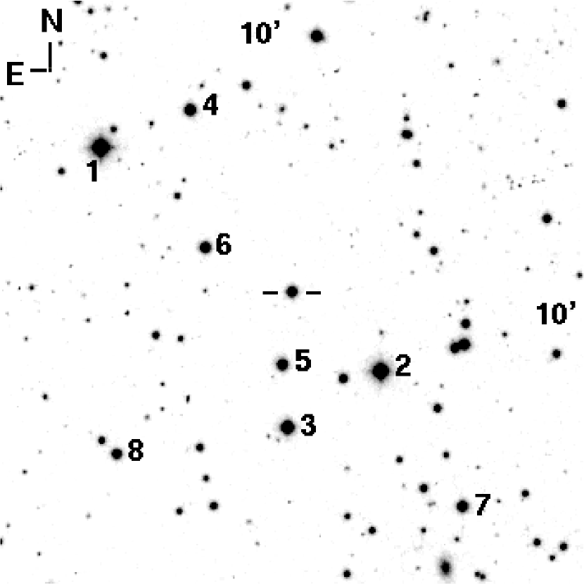
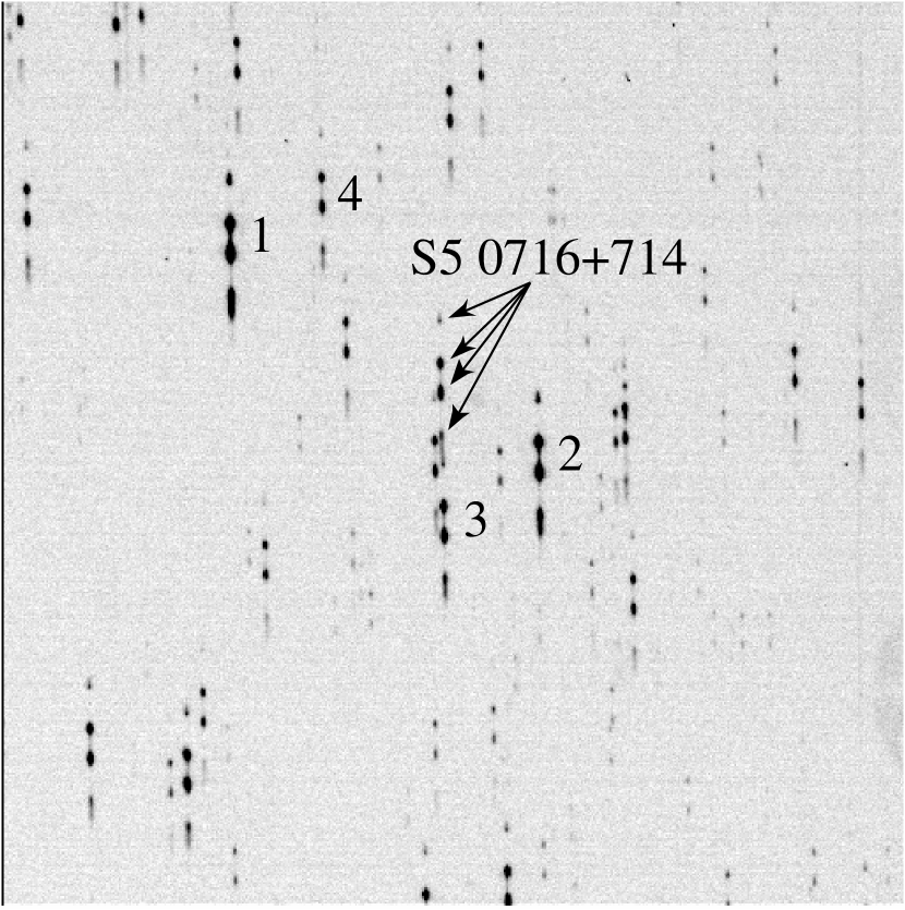
Figure 2: Finding chart of S5 0716+714 (left) and example CCD frame (right) taken with the novel photometric system. The sizes are $10\arcmin\times 10\arcmin$ and $14\farcm 5\times 14\farcm 5$, respectively. Labeled on the finding chart are the BL Lac object and eight reference stars. The first four stars are used to calibrate the BL Lac. Each object has four images on the frame, as indicated for S5 0716+714. For those faint sources, only two central images are visible.

Figure 2 shows the finding chart of S5 0716+714 and an example CCD frame taken with this novel photometric system. Each source now has four “images” (actually four segments in the spectrum of the objective prism) on the frame. The four images, from bottom to top, correspond to the four peaks, from left to right, in Figure 1. Because of the lower CCD responses and filter transmissions at the first and fourth peaks, the first and the fourth images are much fainter than the second and third ones. For the faint objects, only the second and third images are visible. Therefore, in the current paper, we do not use the data in the first and fourth passbands in the scientific analyses, but show two example light curves in the blue band. In the near future, a new thin CCD will be mounted to the telescope. It has much higher responses in the blue wavelengths, so we will have simultaneous photometries in at lease three passbands then.

The monitoring of S5 0716+714 with this novel photometric system covered the period from 2006 January 1 to February 1. As a result of weather conditions, there are actually 19 nights’ data in total. The exposure time ranges from 120 to 540 s, depending on the weather and moon phase. A histogram of the exposure time is shown in Figure 3. One can see that the majority of the exposure times do not exceed 300 s. The readout time is about 5.6 s. So we have achieved a very high temporal resolution in multi wavebands with this new photometric system. The observational log and parameters are presented in Table 2.

2.3 Data Reduction Procedures

The procedures of data reduction include positional calibration, bias subtraction, flat-fielding, extraction of instrumental aperture magnitude, and flux calibration. The positional calibration was made for the $R^{\prime}$-band image, and the “coordinates” of the $V^{\prime}$- and $B^{\prime}$-band images were known by their relative positions to their corresponding $R^{\prime}$-band images. The “coordinates” in the $V^{\prime}$ and $B^{\prime}$ bands are, of course, not the coordinates in the common sense but are only labels for us to find the images during the photometry. The bias subtraction and flat-fielding were done as for the normal CCD frames.

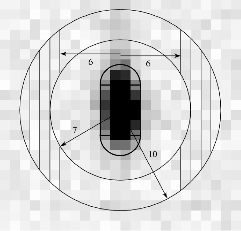
Figure 4: Aperture and sky annulus definitions for an example image on a frame. The traditional circular aperture is cut into two semi-circles along the RA direction, and a rectangle is inset into them. An elongated aperture is thus obtained. Images in different colors have different sizes of rectangles and semi-circles. The shaded areas in the annulus are taken to be the sky background. See text for details.

All images are elongated in the declinational direction, especially for the $B^{\prime}$-band images. So apertures with special shapes were defined for them and are illustrated in Figure 4. The traditional circular aperture is cut into two semi-circles along the RA direction, and a rectangle is inset into them. An elongated aperture is thus obtained. For the $V^{\prime}$- and $R^{\prime}$-band images, the widths of the rectangles (or the diameters of the semi-circles) are both 4 pixels, but the heights are 5 and 4 pixels, respectively. For the $B^{\prime}$-band image, the width and height of the rectangle are 3 and 14 pixels, respectively. All images have a sky annulus definition with inner and outer radii as 7 and 10 pixels, respectively. In order to eliminate the possible contamination of the apertures to their background, areas within 6 pixels in RA to the aperture center are excluded, and only the shaded areas are taken to be the actual sky background.

Villata et al. (1998) presented eight reference stars around S5 0716+714, as labeled in the left panel of Figure 2. We used the first four to calibrate S5 0716+714. Their broadband $B$, $V$, and $R$ magnitudes were used to mimic their standard $B^{\prime}$, $V^{\prime}$, and $R^{\prime}$ ones during the calibrations. The results are presented in Table 2. The columns are observation date and time (UT), Julian Date, exposure time, and $B^{\prime}$, $V^{\prime}$, and $R^{\prime}$ magnitudes, their errors, and the differential magnitudes of reference stars. The differential magnitude of reference stars is defined as the magnitude difference (nightly mean set to 0) between star 3 and the average of the first four. It can be taken as a measure of the accuracy of the observations.

There are, of course, some systematic differences between our $B^{\prime}$, $V^{\prime}$, and $R^{\prime}$ system and the broadband $B$, $V$, and $R$ system. To quantitatively assess the differences, we carried out photometric measurements for seven reference stars (1, 2, 3, 4, 6, 7, 8) by using the same aperture and background definitions and by using the same four reference stars for flux calibrations, as exactly did for S5 0716+714. Star 5 was excluded because its $R^{\prime}$ image is partly overlapped with the $B^{\prime}$ image of the BL Lac and its $B^{\prime}$ image is very close to the $V^{\prime}$ and $R^{\prime}$ images of star 3. The photometric measurements of the seven stars were carried out for 20 best-observed frames taken on the photometric night of JD 2,453,742. Then the average $B^{\prime}$, $V^{\prime}$, and $R^{\prime}$ magnitudes were calculated for the seven stars and compared with their $B$, $V$, and $R$ magnitudes. The standard deviations of 7 $(B-B^{\prime})$’s, 7 $(V-V^{\prime})$’s, and 7 $(R-R^{\prime})$’s were computed, and the results are 0.048, 0.028, and 0.036 mags, respectively. This indicates that there are only small systematic difference between our $B^{\prime}$, $V^{\prime}$, and $R^{\prime}$ system and the broadband $B$, $V$, $R$ system.

3 RESULTS

3.1 Light Curves

The $V^{\prime}$- and $R^{\prime}$-band light curves of the whole monitoring period are shown in Figure 5. The object was very active during this period. Two strong flares can be seen at JD 2,453,742 and 2,453,757 with amplitudes of about 0.8 and 0.6 mags, respectively. Additional flares might also occur at JD 2,453,738, 2,453,745, and/or 2,453,749. The latter three are less certain because of the lack of observations on one or both sides of them. In addition to the strong internight variations, one can see clear intranight variations as well. Except for those less sampling nights (JD 2,453,745, 2,453,760, and 2,453,768), most intranight amplitudes are larger than 0.1 mags and can be as large as 0.3 mags.

The whole light curve can be divided into two halves. Statistically, the first half has larger amplitudes in both internight and intranight variations than the second half has. So the object was more active in the first half than in the second.

Figure 6 gives the intranight light curves on JD 2,453,737 and 2,453,742, which are respectively the first and the brightest nights. From top to bottom, they are in $B^{\prime}$, $V^{\prime}$, and $R^{\prime}$ bands, respectively. The large panels are the light curves of S5 0716+714, while the small ones give the differential magnitudes (nightly mean set to 0) between star 3 and the average of the first four.

On JD 2,453,737, the object kept on brightening, with some oscillations, then got fainter at the end. There was a sharp increase in brightness around JD 2,453,737.26. The $V^{\prime}$ magnitude increased from 12.949 at JD 2,453,737.26147 to 12.886 at JD 2,453,737.27124 (see Table 2), resulting in a brightening rate of about 0.004 $\rm{mag\,min^{-1}}$, which is twice as fast as the rate reported by Villata et al. (2000). On JD 2,453,742, the object underwent some small-amplitude oscillations at first. Then a flare was observed with an amplitude of about 0.235 mags in the $V^{\prime}$ band and a duration of about 0.2 days. The flare peaks at JD 2,453,742.31079. It is also the peak of the first strong flare that lasted for five days (see Fig. 5).

As can be seen, our temporal resolution is very high. The typical sampling intervals are $3.5\sim 4.0$ minutes in these two nights. On both nights, the light curves in the three bands are consistent excellently with each other, and the differential magnitudes in the $V^{\prime}$ and $R^{\prime}$ bands have small rms’s (0.0089 and 0.0093 for JD 2,453,737, and 0.0088 and 0.0103 for JD 2,453,742), which both signify the accuracy of our observations. As expected, the $B^{\prime}$-band data have large errors (for clarity, the error bars are not plotted), and the curves show frequent, irregular jumps in both large and small panels. So we did not show the $B^{\prime}$ band light curve in Figure 5, and will not use the $B^{\prime}$ band data in the following analyses.

3.2 Correlations and Time Lags

In order to investigate the correlation between the variations in different wave bands and to derive the possible lags between them, we at first carried out analyses of the z-transformed discrete correlation function (ZDCF; Alexander, 1997) on the $V^{\prime}$- and $R^{\prime}$-band variations. The ZDCFs between the $V^{\prime}$- and $R^{\prime}$-band variations are presented in Figure 7 for JD 2,453,737 and 2,453,742. The dashed lines are Gaussian fits to the points, and the dotted lines label the centers of the Gaussian profiles, which signify the time lags of the $R^{\prime}$-band to the $V^{\prime}$-band variations. The lags are $1.27\pm 0.22$ and $0.06\pm 0.18$ minutes for JD 2,453,737 and 2,453,742, respectively.

At the same time, the interpolated cross-correlation function (ICCF; Gaskell & Peterson, 1987) was used to measure the time lags and the errors. The error was estimated with a model-independent Monte Carlo method, and the lag was taken as the centroid of the cross-correlation functions that were obtained with a large number of independent Monte Carlo realizations (White & Peterson, 1994; Peterson et al., 1998, 2004). Four thousand realizations were performed for both nights and gave the lags as $2.34\pm 5.27$ on JD 2,453,737 and $-0.01\pm 1.88$ minutes on JD 2,453,742.

All time lags are very short, shorter than our typical sampling interval, and are associated with large errors. So we conclude that our observations do not detect apparent time lag between the $V^{\prime}$- and $R^{\prime}$-band variations.

In optical regimes, variations at long wavelengths are usually reported to lag those at short wavelengths. For S5 0716+714, Qian, Tao, & Fan (2000) determined an upper limit of lag of about 6 minutes between the $V$ and $I$ band variations. Similarly, Villata et al. (2000) claimed an upper limit of 10 minutes to the possible delay between the $B$ and $I$ band variations using high quality data. Most recently, Stalin et al. (2006) reported time lags of about 6 and 13 minutes for the $V$ and $R$ band variations on two individual nights. But they also noted that their measurement intervals were close to these putative lags, and the lags should be treated with caution. For other objects, for example, Romero, Cellone, & Combi (2000) detected time lags of a few to 17.3 minutes between the $V$ and $R$ band variations for PKS 0537$-$441. However, the monitoring on 3C 66A does not strongly support any time lag between variations at different wavelengths. The detailed spectral modeling with a time-dependent leptonic one-zone jet model also does not predict such spectral hysteresis (M. Böttcher, private communication). Our data, characterized by very high temporal resolution and simultaneous measurements in multi frequencies, do not detect apparent lag between variations in the $V^{\prime}$ and $R^{\prime}$ bands. Compared to the much longer lags between variations in X-rays (e.g., Takahashi et al., 1996, $\sim 1$ hr) or between X-ray and EUV/UV variations (e.g., Urry et al., 1997, $1\sim 2$ days), these very short or even absent time lags in optical regimes may be the result of very small frequency intervals, and may indicate that the photons in these wavelengths should be produced by the same physical process and emitted from the same spatial region.

3.3 Color Behavior

3.3.1 The Color-Magnitude Correlation

As mentioned in §1, the color behavior during the variations can put strong constraints on the variation mechanisms. Figure 8 displays the color versus magnitude distributions on JD 2,453,737 and 2,453,742. There is a clear bluer-when-brighter (BWB) chromatism on both nights. The dashed lines are linear fits to the points. The Pearson correlation coefficients are 0.368 and 0.444, and the significance levels are $1.1\times 10^{-6}$ and $1.6\times 10^{-8}$, respectively, which indicate strong correlations between color and magnitude. The dashed lines have slopes of 0.060 and 0.076 for JD 2,453,737 and 2,453,742, respectively.

For all nights, there is also a BWB trend for S5 0716+714. This is illustrated in Figure 9. The dashed line is the linear fit to the 1815 points, and it has a slope of 0.061. The Pearson correlation coefficient is 0.552, indicating a strong correlation between the color and magnitude.

The color or spectral behaviors of S5 0716+714 and other blazars have been investigated in optical bands by many authors (Vagnetti, Trevese, & Nesci, 2003; Stalin et al., 2006; Wu et al., 2005, and references therein). On short timescales, the blazars usually BWB chromatism when they are in an active or flaring state. On long timescales, an achromatic trend is usually found. Our intranight color behavior is in agreement with previous results, whereas the long-term internight variations show a different color behavior. Our BWB chromatisms argue strongly against the microlensing or geometrical effects as the variation mechanisms in S5 0716+714.

In the variability of blazars, two factors may result in color change. One is the difference in variation steps at different frequencies, and the other, the difference in variation amplitudes of these variations. If the variation at high frequency leads that at low frequency, we will observe a BWB chromatism. On the other hand, if the fluxes at different frequencies vary simultaneously, but the amplitude is larger at high frequency than at low one, we will again observe a BWB chromatism. In the actual cases, it may be a combination of these two factors that results in the color changes of blazars. In §3.2, we do not find apparent time lag between variations in different wave bands. The observed BWB phenomena should be mainly attributed to the larger amplitudes at higher frequency This will be confirmed in the next section.

3.3.2 Color-Activity Correlation

The bottom panel of Figure 5 displays the temporal evolution of the color $V^{\prime}-R^{\prime}$ or the $V^{\prime}-R^{\prime}$ “color curve”. Most nights have a scatter less than 0.1 in color, except for JD 2,453,749 and 2,453,754. The two nights are close to or within the phase of full moon, so the photometries have relatively larger errors, and the colors are much more scattered than those in other nights.

From the color curve, one can see that the object generally showed a bluer color when it was brighter, which is consistent with the result in Figure 9. However, it is also clear that the color does not correlate solely with the brightness. For example, the object was brightest but not bluest on JD 2,453,742. The brightness on JD 2,453,737, 2,453,738, and 2,453,740 is much fainter than that on JD 2,453,742, but the former nights have comparable or even bluer colors than the latter night has. In analogy to the division of the light curve, the color curve can also be divided into two halves, i.e., those before and after JD 2,453,750. The first half is much bluer than the second, as manifested by the dashed line, the mean color, in the color curve in the bottom panel of Figure 5. Therefore, the object seems show a bluer color when it is more active.

To study the relation between the color and the activity in more detail, we at first need to define the activity of a blazar, or how a blazar is called active. The activity has two aspects; one is the frequency or rate, and the other, the amplitude. The frequency of activity can be described by duty cycle, which is defined as the fraction of time a source spends more than $3\sigma$ away from its weekly average (Wagner & Witzel, 1995).

For the amplitude of activity, we define it as the sum of the intranight and internight amplitudes

$$A=A_{\rm intran}+A_{\rm intern}.$$ (1)

The intranight amplitude can be simply calculated as the difference between the maximum and minimum magnitudes (or fluxes) of a certain night, as did in §3.1.3. A more precise way is to take the measurement error into account. As in Heidt & Wagner (1996), the intranight amplitude is defined as

$$A_{\rm intran}=\sqrt{(m_{\rm max}-m_{\rm min})^{2}-2\sigma^{2}},$$ (2)

where $m_{\rm max}$ and $m_{\rm min}$ are respectively the maximum and minimum magnitudes (or fluxes) of a certain night, and $\sigma$ is the measurement error. Here we take $\sigma$ as the nightly average of the differential magnitude of reference stars ($\delta V^{\prime}$ or $\delta R^{\prime}$ in Table 2).

For the internight amplitude, the average magnitudes (or fluxes) are calculated at first for all nights. Then the internight amplitude of the $i$th night is defined as

$$A_{{\rm intern},i}=\frac{|\langle m\rangle_{i}-\langle m\rangle_{i-1}|+|\langle m\rangle_{i}-\langle m\rangle_{i+1}|}{2},$$ (3)

where $\langle m\rangle_{i-1}$, $\langle m\rangle_{i}$, and $\langle m\rangle_{i+1}$ are the average magnitudes of the $(i-1)$th, $i$th, and $(i+1)$th nights. When there is no observation on the $(i-1)$ or $(i+1)$ night, the data on the night closest to the $(i-1)$ or $(i+1)$ night are used if the time differences are not large, but the resulting amplitude may have large error. For the first and the last night of the sequence, only the first or second absolute value is calculated in Equation 3 and it is not divided by 2. In this paper, we will focus on the amplitude rather than the frequency of activity. So we call a blazar “active” when it has a large amplitude of activity.

With these definitions, we calculated the intranight and internight amplitudes of activity of S5 0716+714 on the 19 monitoring nights and listed the results in Table 3. The columns are Julian Date, average $V^{\prime}$ magnitude, internight and intranight amplitudes in the $V^{\prime}$ band, average $R^{\prime}$ magnitude, internight and intranight amplitudes in the $R^{\prime}$ band, and time duration of the monitoring in that night. Figure 10 illustrates the relation between the color and the amplitude of activity. We do not plot the data on JD 2,453,749 and 2,453,754 because they have much larger measurement errors and much larger scatters in color than those on other nights. Data on JD 2,453,745, 2,453,760, and 2,453,768 are also excluded from the figure because they are much less sampled than those on other nights. So there are 14 nights’ data left. The triangles and circles designate nights of the first and second halves of the light curve, respectively. The former has much bluer color than the latter, as expected. The solid line is the best fit to the 14 points. The Pearson correlation coefficient is $-0.851$ and the significance level is $1.15\times 10^{-4}$, which mean strong correlation between color and amplitude of activity. The correlation confirms the result of the above visual inspection: the object showed a bluer color when it was more active.

Figure 11 displays whether the intranight and internight amplitudes separately correlate with the color. The distribution on the left panel has a Pearson correlation coefficient of $-0.745$ and a significance level of $2.24\times 10^{-3}$, while the right panel shows a correlation coefficient of $-0.576$ and a significance level of 0.03. The former correlation is stronger than the latter, but they are both much weaker than the correlation in Figure 10.

Most observations detected a BWB chromatism in blazars. At the same time, a minority of monitorings found a redder-when-brighter trend in some blazars (e.g., Raiteri et al., 2003; Gu et al., 2006). This inconsistency may be explained with the bluer-when-more-active (BWMA) chromatism: even though the object is in a faint state, it can still have relatively large amplitude of variations, so it can show a relatively blue color.

4 COLOR EVOLUTION DURING THE FLARE

According to theoretical predictions, the color of a blazar usually evolves with a wave-like pattern during a flare, and there is usually a loop path on the color versus magnitude (or flux) diagram, in either clockwise or anti-clockwise direction. The direction depends on the frequency that the observation is made and the peak frequency of the synchrotron component in the spectral energy distribution (SED) of the blazar (see Figs. 3 and 4 in Kirk, Rieger, & Mastichiadis, 1998). The loop path has been frequently observed in X-ray (e.g., Sembay et al., 1993; Takahashi et al., 1996; Kataoka et al., 2000; Zhang et al., 1999, 2002; Malizia et al., 2000; Ravasio et al., 2004), and, in one case, in infrared (Gear, Robson, & Brown, 1986). In optical regimes, only Xilouris et al. (2006) have reported a similar pattern.

In our monitoring, we recorded two strong flares, i.e., the one from JD 2,453,740 to 2,453,744 and the other from JD 2,453,754 to 2,453,760 (see Fig. 5). The temporal evolutions of the color do follow a wave-like pattern during the two flares (see the bottom panel of Fig. 5). On the color versus magnitude diagrams in Figure 12, the results are controversial. When the individual measurements are considered, both diagrams are just messy; when we focus only on the nightly means, there is a loop in clockwise direction on both diagrams, as labeled by the arrows.

The loop path can be explained by a spectral hysteresis, i.e., the variation in one band lags that in the other. Our observations do not find apparent time lags between the intranight variations in different wave bands, so the individual measurements do not show a loop path. However, the loop paths described by the nightly means may suggest that S5 0716+714 has a spectral hysteresis in its long-term (from hours to days) variations. By using the same Monte Carlo algorithm of White & Peterson (1994) and Peterson et al. (1998, 2004), we derived a time lag of $0.10\pm 3.98$ days between the $V^{\prime}$- and $R^{\prime}$-band nightly-mean light curves. Given the large error and the short lag relative to the sampling interval (1 day), the result is of relatively low significance level in quantity, but should be qualitatively reasonable.

5 CONCLUSIONS AND DISCUSSIONS

In this paper, we have introduced a novel photometric system, which consists of a Schmidt telescope, an objective prism, a CCD camera, and, especially a multi-peak interference filter. The multi-peak interference filter enables light in multi passbands to pass through it simultaneously. The light in different passbands are differentially refracted by the objective prism and focus on the CCD separately, so we have multi images for each object on the CCD frames. This system enables us to carry out simultaneous photometric measurements in multi wavebands, and it has the advantage of being invulnerable to the possible instability of instruments and weather. When using for blazar monitorings, the system can accurately trace the color change during the variation, which is crucial in constraining the variation mechanisms of blazars.

The multi-peak interference filter is new, at least in blazar monitorings. The transition from the traditional one-passband filter to the new multi-peak interference filter is analogous to the transition from the traditional slit spectrograph to the fiber spectrograph. The new filter can greatly increase the efficiency of data sampling and is worthy being extended to the observations of other targets, especially those variable sources.

This novel photometric system was used in the monitoring of S5 0716+714 and we achieved a very high temporal resolution. The BL Lac object was very bright and very active during our monitoring period and showed strong variations on both internight and intranight timescales. Two strong flares were observed, with amplitudes of variations of about 0.8 and 0.6 mags, respectively. There may be three more but less certain flares. Significant BWB correlations were found for both internight and intranight variations, and the BWB internight variability is different from the basically achromatic long-term variability of S5 0716+714 observed previously (Ghisellini et al., 1997; Raiteri et al., 2003). No apparent time lag was found between the $V^{\prime}$- and $R^{\prime}$-band variations. The BWB chromatism should be mainly attributed to the larger amplitude of variation at higher frequency.

In addition to the BWB chromatism, we also found a BWMA chromatism, which is new and has not been reported before. It helps to explain some exceptional color behaviors (e.g., redder-when-brighter) observed in blazars sometimes. The theoretical reason for the BWMA chromatism is still unknown. Phenomenologically, when the object is more active (has larger variation amplitude), the difference in variation amplitudes in different wavebands is larger, so the object is bluer. Unlike the BWB chromatism, which can be either long- or short-term behavior, the BWMA phenomenon is only a long- or, at least, intermediate-term behavior. To reveal or confirm the BWMA chromatism, the monitoring should cover a relatively long period and consists of as many successive nights as possible. Intensive intranight observations are also desired.

The color behaviors can put strong constraints to the variation mechanisms of blazars. The mechanisms can be broadly classified into extrinsic and intrinsic origins (Wagner & Witzel, 1995). The extrinsic origins include the ISS and gravitational microlensing effects. The ISS can explain variations at low radio frequencies, but can not produce variations at optical wavelengths. The microlensing is an achromatic process and should result in strictly symmetric light curves, which are both contrary to our results. So the variations of S5 0716+714 observed by us are unlikely to have an extrinsic origin. The intrinsic origins include the shock-in-jet scenario, accretion disk instability, and geometrical effects. In the accretion disk scenario, external gravitational perturbations may induce flares and hot spots in the accretion disk around a black hole. This may account for the optical-UV microvariability observed in blazars (Chakrabarti & Wiita, 1993; Mangalam & Wiita, 1993), but it has difficulty in explaining the strong or rapid flares in blazars, as observed by us. It also can not account for the correlated radio-optical variations observed in S5 0716+714 (Quirrenbach et al., 1991). In fact, the general absence of the big blue bump in the SED of blazars also argue against a significant contribution of the thermal emission from the accretion disk to the overall emission of blazars. The geometrical effects are that the helical or precessing jet leads to varying Doppler boosting towards the observers and hence the flux variations. They usually result in achromatic and periodic variations, which is also not the case in our results. Now the other mechanisms are all excluded, the shock-in-jet scenario becomes most plausible. In fact, the irregular variations and, especially, the BWB color behaviors are all consistent with the predictions of the shock-in-jet model.

Variation mechanism is an essential issue in the investigations of blazars. Our new photometric system has the advantages of accurate color trace, high temporal resolution, and being invulnerable to instrumental and weather instabilities. A new thin CCD camera will soon be mounted to the telescope, and it has much higher responses in blue wavelengths than the current thick CCD has. The objective prism may also soon be replaced by an diffraction grating. The upgraded system will be used to monitor a few bright blazars in the near future, and the simultaneous three-band photometries will help to investigate the variation mechanisms in them with high confidence level.

Figure 1: Transmission curve of the multi-peak interference filter.

Figure 3: Histogram of exposure time. Most exposure times are equal to or less than 300 s.

Figure 5: Light curves in the $V^{\prime}$ and $R^{\prime}$ bands and color evolution. The first halves of the light curves have much larger amplitudes in both internight and intranight variations than the second halves. The colors in the first half is much bluer than those in the second, as manifested by the dashd line, the mean color.

Figure 6: Intranight light curves on JD 2,453,737 and 2,453,742, in $B^{\prime}$, $V^{\prime}$, and $R^{\prime}$ bands from top to bottom. The large panels show the light curves of S5 0716+714, while the small ones display the differential magnitudes between star 3 and the average of the first four. The errors are not plotted for clarity. The $B^{\prime}$ band light curves have large errors, as can be seen in the small panels.

Figure 7: ZDCFs between the $V^{\prime}$- and $R^{\prime}$-band variations on JD 2,453,737 and 2,453,742. The dashed lines are Gaussian fits to the points, and the dotted lines (at 1.27 and 0.06 minutes for left and right, respectively) label the centers of the Gaussian profiles, which signify the lags of the $R^{\prime}$ band to $V^{\prime}$ band variations.

Figure 8: Color versus magnitude distribution for JD 2,453,737 and 2,453,742. The dashed lines are linear fits to the points. The Pearson correlation coefficients of 0.368 and 0.444 indicate strong correlations between color and magnitude. The slopes of the two fits are 0.060 and 0.076, respectively.

Figure 9: Color versus magnitude distribution for all nights. The linear fit to the points, the dashed line, gives a slope of 0.061. The Pearson correlation coefficient of 0.552 means a strong correlation between color and magnitude.

Figure 10: Correlation between color and amplitude of activity. The triangles are nights of the first half of our monitoring period, whereas the open circles are nights of the second half. The solid line is the best fit to all 14 points. The Pearson correlation coefficients, $r=-0.851$, indicate a strong trend that the object become bluer when it is more active.

Figure 11: Correlations between color and intranight (left) and internight (right) amplitudes. The former correlation is stronger than the latter, but both are much weaker than the correlation in Fig. 10.

Figure 12: Color versus magnitude distributions during two flares. Different symbols signify measurements on different nights. The individual measurements do not describe a loop path, while the nightly means define two loop paths in clockwise direction, as indicated by the arrows.

Table 1: Parameters of the Left Three Passbands of the Filter

Passband	Wavelength	Max Trans	FWHM
	(Å)	(%)	(Å)
$B^{\prime}$	4575.2	59.40	355
$V^{\prime}$	5672.9	88.28	210
$R^{\prime}$	6786.6	58.34	162

Table 2: Observational log and results in the $B^{\prime}$, $V^{\prime}$, and $R^{\prime}$ bands.

Date	Time	Julian Date	Exp.	$B^{\prime}$	$B^{\prime}_{\rm err}$	$\delta B^{\prime}$	$V^{\prime}$	$V^{\prime}_{\rm err}$	$\delta V^{\prime}$	$R^{\prime}$	$R^{\prime}_{\rm err}$	$\delta R^{\prime}$
			(s)	(mag)	(mag)	(mag)	(mag)	(mag)	(mag)	(mag)	(mag)	(mag)
2006 01 01	11:30:07	2453736.97925	240	13.463	0.027	0.022	13.081	0.009	0.009	12.662	0.009	$-$0.014
2006 01 01	11:49:27	2453736.99268	180	13.476	0.027	0.039	13.072	0.011	0.019	12.644	0.012	0.000
2006 01 01	11:54:06	2453736.99585	180	13.521	0.031	0.061	13.059	0.010	$-$0.018	12.628	0.011	$-$0.006
2006 01 01	12:30:03	2453737.02075	180	13.497	0.026	0.053	13.051	0.010	$-$0.010	12.597	0.010	$-$0.006
2006 01 01	12:33:27	2453737.02319	180	13.531	0.028	$-$0.015	13.045	0.010	0.000	12.619	0.009	0.011

Note. — Table 2 is published in its entirety in the electronic edition of the Astronomical Journal. A portion is shown here for guidance regarding its form and content.

Table 3: Average Magnitudes and Variation Amplitudes on Individual Nights

Julian Date	$\langle V^{\prime}\rangle$	$A_{\rm V^{\prime},intern}$	$A_{\rm V^{\prime},intran}$	$\langle R^{\prime}\rangle$	$A_{\rm R^{\prime},intern}$	$A_{\rm R^{\prime},intran}$	Duration
	(mag)	(mag)	(mag)	(mag)	(mag)	(mag)	(day)
2453737	12.952	0.182	0.302	12.533	0.186	0.298	0.444
2453738	12.770	0.275	0.199	12.347	0.263	0.202	0.403
2453740	13.138	0.380	0.098	12.688	0.350	0.091	0.317
2453741	12.746	0.302	0.269	12.329	0.289	0.246	0.423
2453742	12.533	0.207	0.278	12.109	0.201	0.251	0.421
2453743	12.733	0.181	0.095	12.292	0.168	0.084	0.411
2453744	12.895	0.162	0.174	12.446	0.154	0.143	0.429
2453745	12.691	0.204	0.055	12.257	0.189	0.049	0.076
2453749	13.062	0.186	0.242	12.606	0.179	0.212	0.223
2453754	13.063	0.044	0.077	12.614	0.053	0.075	0.359
2453756	12.977	0.160	0.151	12.516	0.150	0.131	0.196
2453757	12.817	0.117	0.191	12.366	0.110	0.184	0.402
2453758	12.892	0.135	0.103	12.436	0.125	0.096	0.420
2453759	13.087	0.162	0.142	12.617	0.160	0.122	0.334
2453760	13.171	0.065	0.055	12.712	0.070	0.055	0.087
2453761	13.216	0.069	0.179	12.756	0.074	0.161	0.417
2453762	13.226	0.052	0.160	12.764	0.047	0.151	0.405
2453767	13.320	0.094	0.116	12.849	0.085	0.128	0.409
2453768	13.387	0.067	0.065	12.915	0.066	0.046	0.026

References

- Abramowicz et al. (1991) Abramowicz, M. A., Bao, G., Lanza, A., & Zhang, X.-H. 1991, A&A, 245, 454
- Alexander (1997) Alexander, T. 1997, in Astronomical Time Series, ed. D. Maoz, A. Sternberg, & E. M. Leibowitz (Dordrecht: Kluwer), 163
- Camenzind & Krockenberger (1992) Camenzind, M. & Krockenberger, M. 1992, A&A, 255, 59
- Chakrabarti & Wiita (1993) Chakrabarti, S. K. & Wiita, P. J. 1993, ApJ, 411, 602
- Dolcini et al. (2005) Dolcini, A., et al. 2005, A&A, 443, L33
- Fiedler et al. (1987) Fiedler, R., Dennison, B., Johnston, K. J., & Hewish, A. 1987, Nature, 326, 675
- Gaskell & Peterson (1987) Gaskell, C. M. & Peterson, B. M. 1987, ApJS, 65, 1
- Gear, Robson, & Brown (1986) Gear, W. K., Robson, E. I., & Brown, L. M. J. 1986, Nature, 324, 546
- Ghisellini et al. (1997) Ghisellini, G., et al. 1997, A&A, 327, 61
- Gu et al. (2006) Gu, M. F., Lee, C.-U., Pak, S., Yim, H. S., & Fletcher, A. B. 2006, A&A, 450, 39
- Heidt & Wagner (1996) Heidt, J. & Wagner, S. J. 1996, A&A, 305, 42
- Kataoka et al. (2000) Kataoka, J., Takahashi, T., Makino, F., Inoue, S., Madejski, G. M., Tashiro, M., Urry, C. M., & Kubo, H. 2000, ApJ, 528, 243
- Kirk, Rieger, & Mastichiadis (1998) Kirk, J. G., Rieger, F. M., & Mastichiadis, A. 1998, A&A, 333, 452
- Liu & Wu (2002) Liu, F. K. & Wu, X. B. 2002, A&A, 338, L48
- Malizia et al. (2000) Malizia, A. et al. 2000, MNRAS, 312, 123
- Mangalam & Wiita (1993) Mangalam, A. V. & Wiita, P. J. 1993, ApJ, 406, 420
- Marscher & Gear (1985) Marscher, A. P., & Gear, W. K. 1985, ApJ, 298, 114
- Montagni et al. (2006) Montagni, F., Maselli, A., Massaro, E., Nesci, R., Sclavi, S., & Maesano, M. 2006, A&A, 451, 435
- Nesci, Massaro, & Montagni (2002) Nesci, R., Massaro, E., & Montagni, F. 2002, Publ. Astron. Soc. Aust. 19, 143
- Nottale (1986) Nottale, L. 1986, A&A, 157, 383
- Peterson et al. (1998) Peterson, B. M., Wanders, I., Horne, K., Collier, S., Alexander, T., Kaspi, S., & Maoz, D. 1998, PASP, 110, 660
- Peterson et al. (2004) Peterson, B. M., et al. 2004, ApJ, 613, 682
- Qian et al. (1991) Qian, S. J., Quirrenbach, A., Witzel, A., Krichbaum, T. P., Hummel, C. A., & Zensus, J. A. 1991, A&A, 241, 15
- Qian, Tao, & Fan (2000) Qian, B., Tao, J., & Fan, J. 2000, PASJ, 52, 1075
- Quirrenbach et al. (1991) Quirrenbach, A., Witzel, A., Wagner, S., et al. 1991, ApJ, 372, L71
- Raiteri et al. (2003) Raiteri, C. M., Villata, M., Tosti, G. et al. 2003, A&A, 402, 151
- Ravasio et al. (2004) Ravasio, M., Tagliaferri, G., Ghisellini, G., & Tavecchio, F. 2004, A&A, 424, 841
- Rickett et al. (2001) Rickett, B. J., Witzel, A., Kraus, A., Krichbaum, T. P., & Qian, S. J. 2001, ApJ, 550, L11
- Romero, Cellone, & Combi (2000) Romero, G. E., Cellone, S. A., & Combi, J. A. 2000, AJ, 120, 1192
- Schneider & Weiss (1987) Schneider, P., & Weiss, A. 1987, A&A, 171, 49
- Sembay et al. (1993) Sembay, S., Warwick, R. S., Urry, C. M., Sokoloski, J., George, I. M., Makino, F., Ohashi, T., & Tashiro, M. 1993, ApJ, 404, 112
- Sillanpää et al. (1988) Sillanpää, A., Haarala, S., Valtonen, M. J., Sundelius, B., & Byrd, G. G. 1988, ApJ, 325, 628
- Stalin et al. (2006) Stalin, C. S., Gopal-Krishna, Sagar, R., Wiita, P. J., Mohan, V., & Pandey, A. K. 2006, MNRAS, 366, 1337
- Takahashi et al. (1996) Takahashi, T. et al. 1996, ApJ, 470, L89
- Urry & Padovani (1995) Urry, C. M. & Padovani, P. 1996, PASP, 107, 803
- Urry et al. (1997) Urry, C. M., et al. 1997, ApJ, 486, 799
- Vagnetti, Trevese, & Nesci (2003) Vagnetti, F., Trevese, D., & Nesci, R. 2003, ApJ, 590, 123
- Valtaoja et al. (2000) Valtaoja, E., Teräsranta, H., Tornikoski, M., Sillanpää, A., Aller, M. F., Aller, H. D., & Hughes, P. A. 2000, ApJ, 531, 744
- Villata et al. (1998) Villata, M., Raiteri, C. M., Lanteri, L., Sobrito, G., & Cavallone, M. 1998, A&AS, 130, 305
- Villata et al. (2000) Villata, M., et al. 2000, A&A, 363, 108
- Wagner & Witzel (1995) Wagner, S. J. & Witzel, A. 1995, ARA&A, 33, 163
- White & Peterson (1994) White, R. J. & Peterson, B. M. 1994, PASP, 106, 879
- Wu et al. (2005) Wu, J., Peng, B., Zhou, X., Ma, J., Jiang, Z., & Chen, J. 2005, AJ, 129, 1818
- Xilouris et al. (2006) Xilouris, E. M., Papadakis, I. E., Boumis, P., Dapergolas, A., Alikakos, J., Papamastorakis, J., Smith, N., & Goudis, C. D. 2006, A&A, 448, 143
- Zhang et al. (1999) Zhang, Y. et al. 1999, ApJ, 527, 719
- Zhang et al. (2002) Zhang, Y. et al. 2002, ApJ, 572, 762