Deeply embedded objects and shocked molecular hydrogen: The environment of the FU Orionis stars RNO 1B/1C

Abstract

We present Spitzer IRAC and IRS observations of the dark cloud L1287. The mid–infrared (MIR) IRAC images show deeply embedded infrared sources in the vicinity of the FU Orionis objects RNO 1B and RNO 1C suggesting their association with a small young stellar cluster. For the first time we resolve the MIR point source associated with IRAS 00338+6312 which is a deeply embedded intermediate–mass protostar driving a known molecular outflow. The IRAC colors of all objects are consistent with young stars ranging from deeply embedded Class 0/I sources to Class II objects, part of which appear to be locally reddened. The two IRS spectra show strong absorption bands by ices and dust particles, confirming that the circumstellar environment around RNO 1B/1C has a high optical depth. Additional hydrogen emission lines from pure rotational transitions are superimposed on the spectra. Given the outflow direction, we attribute these emission lines to shocked gas in the molecular outflow powered by IRAS 00338+6312. The derived shock temperatures are in agreement with high velocity C-type shocks.

1 Introduction

The dark cloud L1287 contains the galactic nebulae GN 00.34.0 (associated with the young F-type star RNO 1) and GN 00.33.9 which harbors the IRAS point source IRAS 00338+6312 ($d=800$ pc, Persi et al., 1988). Two young stars, RNO 1B and RNO 1C, lie slightly south-west of the catalog position of the IRAS source. Those objects show properties of FU Orionis objects (FUORs): (1) Staude & Neckel (1991) found that RNO 1B brightened by at least 3 mag over a period of 12 years and that it showed a variable and blueshifted P Cygni profile in H$\alpha$ and additional broad and double–peaked absorption lines in its optical spectrum; (2) Kenyon et al. (1993) obtained near–infrared spectroscopic data for both objects and found the FUOR–typical strong 2.3$\,\mu$m CO absorption bands. As the error ellipse of the IRAS source includes both FUORs it was long debated whether there is still another deeply embedded source close to the FUOR objects or whether IRAS just measured the integrated flux from these two objects. From high–resolution near–infrared (NIR) polarimetric maps Weintraub & Kastner (1993) concluded that an additional embedded object should be present close to the location of the IRAS source. This idea was supported by the discovery of a 3.6 cm continuum peak (Anglada et al., 1994) and an H₂O maser (Fiebig, 1995), both nearly coinciding with the IRAS position. A bipolar outflow in the region was found by Snell et al. (1990) and later confirmed by Yang et al. (1991). As the positions of the IRAS source and the FUORs line up along the outflow axis it has long been uncertain which source was driving the outflow. From interferometric observations in CS Yang et al. (1995) suggested that the IRAS source was most likely the driving source. Recently, Xu et al. (2006) mapped the outflow in CO and came to the same conclusion. However, McMuldroch et al. (1995) presented (sub–)millimeter observations favoring RNO 1C as the outflow driving source.

In this paper we present mid–infrared (MIR) imaging and spectroscopy data taken with the IRAC and IRS instruments onboard the Spitzer Space Telescope. For the first time we resolve the MIR point source associated with the IRAS source and find additional, partly deeply embedded, objects. The two IRS spectra probe the composition of the dense circumstellar environment in the vicinity of RNO 1B/1C and bear additional traces of shocked H₂ gas.

2 Observations and Data Reduction

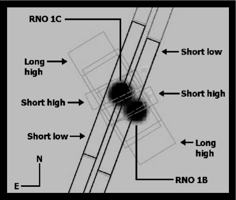
Figure 1: The slits of the different modules of the Spitzer/IRS overplotted on the inverted 2MASS Ks-filter image. The two FUOR objects RNO 1B and RNO 1C are not centered in the slits (north is up, east to the left).

All data were part of the GTO program by R. Gehrz and publicly available from the Spitzer data archive. An overview of the observational setup and the datasets is provided in Table 1. The IRAC images were obtained in sub–array mode leading to an effective field–of–view of  40^′′ centered on the position given in Table 1. The spectra taken with IRS cover the wavelength range $5-37$ $\,\mu$m. Overplotting the spectral slits of IRS on the 2MASS Ks-filter image reveals that apparently RNO 1B and RNO 1C were not centered within the slits (Fig. 1). The short low–resolution spectrum ($5.2-14.5$ $\,\mu$m, R $\sim 64-128$) and the short high–resolution spectrum ($9.9-19.6$ $\,\mu$m, R $\sim 600$) close to RNO 1B seems to probe mainly flux coming from in between the two objects. The spectrum close to RNO 1C contains presumably also less flux than expected due to the slight mispointing. The long high–resolution part in either spectrum ($18.7-37.2$ $\,\mu$m, R $\sim 600$) includes flux from both components and also additional flux from the IRAS source as all three objects lie within the slit of the spectrograph.

The IRAC images were reduced with the MOPEX package provided by the Spitzer Science Center. Interpolation, outlier detection and co–addition of the images were carried out for each filter individually. The astrometry was refined by comparing the position of detected sources to known 2MASS objects. The photometry was carried out with the daophot package provided within the IRAF environment. As there was only a limited number of sources available within the small field covered by the camera we measured the point-spread function (PSF) of RNO 1C and used it as reference to do PSF photometry for all the other sources. Following the IRAC Data Handbook 5.1.1 we converted the pixel values from MJy sr^-1 to DN s^-1 and computed the corresponding magnitudes via $m=-2.5\,log(x)+\Delta_{ZP}$ with $x$ denoting the flux measured in DN s^-1 and $\Delta_{ZP}$ being the zero point for each filter. For the initial PSF fit we used a PSF size of 2 pixel and applied aperture corrections as described in the Data Handbook to obtain the final magnitudes.

Our final IRS spectra are based on the intermediate droopres (for the low–resolution data) and rsc (for the high–resolution data) products processed through the S13.2.0 version of the Spitzer  data pipeline. Partially derived from the SMART software package (Higdon et al., 2004) these intermediate data products were further processed using spectral extraction tools developed by the ”Formation and Evolution of Planetary Systems” (FEPS) Spitzer  science legacy team (see, Explanatory Supplement v. 3.0 within the FEPS data deliveries.

For the short low–resolution observations, the spectra where extracted using a 6.0 pixel fixed-width aperture in the spatial dimension resulting in a 39.96 arcsec² extraction aperture on the sky. The background was subtracted using associated pairs of imaged spectra from the two nodded positions along the slit. This process also subtracts stray light contamination from the peak-up apertures and adjusts pixels with anomalous dark current relative to the reference dark frames. Pixels flagged by the Spitzer  data pipeline as being ”bad” were replaced with a value interpolated from an 8 pixel perimeter surrounding the errant pixel. The high–resolution spectra were extracted with the full aperture size (53.11 arcsec² for the short–high and 247.53 arcsec² for the long–high module). The sky contribution was estimated by fitting a continuum to the data. Both, the low– and high–resolution spectra, are calibrated using a spectral response function derived from IRS spectra appropriate for the two nod positions in the slit at which we extract the specta, and Cohen or MARCS stellar models for a suite of calibrators provided by the Spitzer Science Centre. The multiple orders in our spectra match to within 10%. These small flux offsets are likely related to small pointing offsets. We computed correction factors for possible flux loss due to telescope mispointing based on the PSF of the IRS instrument. However, accurate results can only be obtained if the flux is dominated by one source. The offsets also result in low level fringing at wavlengths longer than 20 micron in the low–resolution spectra and at all wavelengths in the high–resolution spectra. We removed these fringes using the irsfringe package developed by F. Lahuis. The relative errors between spectral points within one order are dominated by the noise on each individual point and not by the calibration. Based on our experience with Spitzer IRS data we estimate a relative flux calibration error across a spectral order of $\approx 5$ % and an absolute calibration error between orders/modules of $\approx 10$ %. These values, however, are based on point source observations with accurate telescope pointing. The data presented here are more complicated as at least part of the emission is moderately extended, multiple sources contribute to the observed fluxes, each contribution is wavelength dependent, and the telescope slits were not centered on the main objects. Thus, an accurate flux calibration between the different modules is difficult and apparent offsets are further discussed in section 3.2.

3 Results

3.1 IRAC photometry

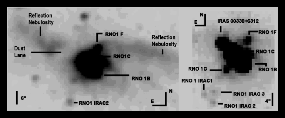
Figure 2: The RNO 1B/1C region in the 2MASS Ks-filter (left) and the 5.8$\,\mu$m IRAC filter (right). The images are inverted and the contrast is set to make also fainter objects visible. The IRAC image contains more sources and especially the IRAS source clearly shows up at 5.8$\,\mu$m while it seems hidden behind a dust lane in the 2MASS image. The magnitudes of the individual sources are listed in Table 2.

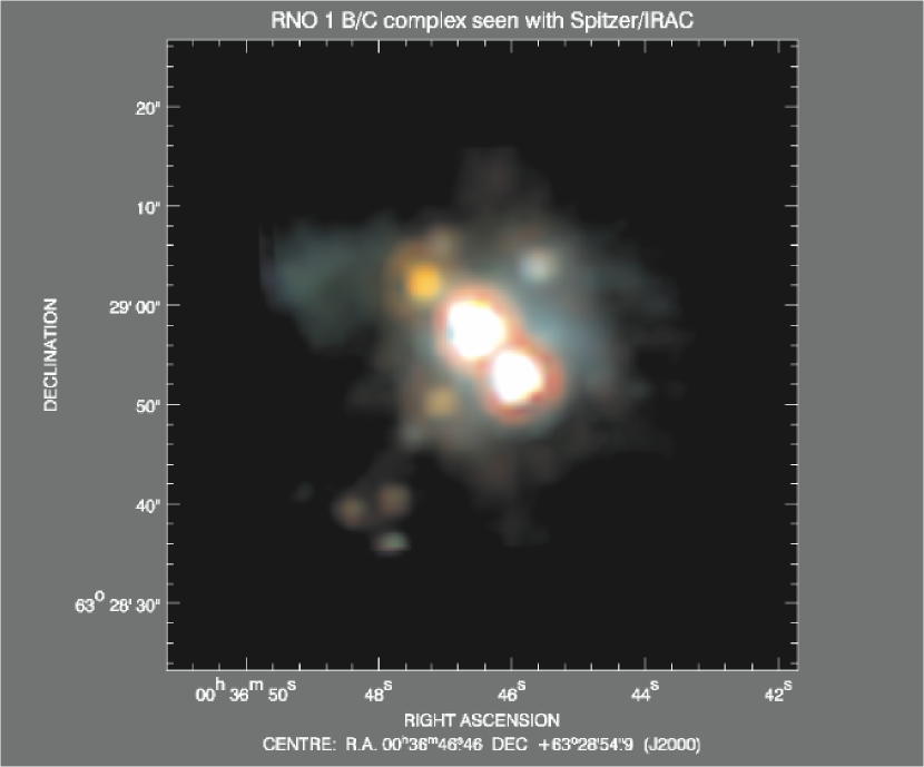
Figure 11: Color composite of the RNO 1B/1C region based on the three IRAC bands at 3.6, 4.5, and 8.0$\,\mu$m. The image is centered on RNO 1C. We applied a logarithmic color stretch to enhance the fainter sources. The extended emission east of the IRAS source which is predominantly seen in the green 4.5$\,\mu$m filter is possibly related to H₂ emission within the bipolar outflow of this object.

Within the limited field–of–view of the IRAC subarray mode we identified 8 sources that were detected in at least three of the four IRAC bands. Figure 2 provides a comparison between the RNO 1B/1C region as seen in the 2MASS Ks-filter and the 5.8$\,\mu$m IRAC filter. For the first time the MIR point source related to IRAS 00338+6312 is detected in the IRAC band. Additional fainter objects are also present, some of which are detected for the first time. Fig. 11 shows a color composite image of the RNO 1B/1C complex based on three IRAC filters. Table 2 lists all objects that were identified in at least three IRAC bands and summarizes the derived fluxes. The errors are based on the results from the PSF-photometry. Since we used the PSF of RNO 1C as reference PSF the corresponding errors are relatively small compared to the other objects.

IRAS 00338+6312 and RNO 1G were not detected in the shortest IRAC band at 3.6$\,\mu$m. The 2MASS image in Fig. 2 shows that at least the IRAS source is deeply embedded in a dense dusty environment explaining the non-detection at this wavelength. Fig. 3 shows two color–color plots based on the four IRAC bands for all objects listed in Table 2. Following Hartmann et al. (2005) who analyzed a large sample of pre-main sequence stars in the Taurus star-forming region we use these plots to classify the different objects. The colors of the reddest objects (IRAS 00338+6312 and RNO 1G) are consistent with very young protostars. The colors of the newly discovered objects RNO1 IRAC1 and RNO1 IRAC3 are consistent with Class 0/I systems although it has to be confirmed that these are indeed nearby objects and not highly reddened background sources. While the colors of the FUOR object RNO 1C fit in the region of Class II objects from Hartmann et al. (2005) in both plots (Fig. 3), RNO 1B fits only in one color-color diagram into this regime. In the right plot of Fig. 3 RNO 1B is too red for a Class II source in the [4.5]-[5.8] color, but not red enough in the [3.6]-[4.5] color to be a Class 0/I object. Finally, RNO1 IRAC 2 and RNO 1F, which both show up in the 2MASS Ks-band image, can also be interpreted as Class II objects. However, the colors of RNO1 IRAC2, but partly also of RNO 1F, are possibly altered due to local extinction effects.

3.2 IRS spectroscopy

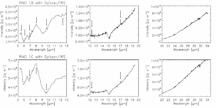
Figure 4: Spitzer/IRS spectra close to RNO 1B (upper row) and RNO 1C (lower row). The leftmost column shows the low–resolution data while the other two columns present the high–resolution spectra. The positions of the H₂-emission lines are indicated by the arrows.

In Figure 4 we show the Spitzer IRS spectra without any extinction correction. As pointed out earlier the spectral slits of the short wavelength modules were apparently not directly centered on the objects RNO 1B and RNO 1C and thus the measured fluxes cannot be attributed to these objects with very high accuracy. Also, there seems to be an offset in the flux in the high–resolution regime compared to the low–resolution part of the spectrum. To see to which extent this effect is caused by different aperture sizes we plotted the spectra in intensities (i.e., flux density per solid angle) rather then in Jansky per wavelength. It shows, however, that even after this correction significant offsets remain: Around 13$\,\mu$m the difference between the low–resolution spectrum and the short high–resolution spectrum amounts to a factor of $\approx$$\,1.25$ and $\approx$$\,1.08$ for RNO 1B and RNO 1C, respectively, with the high–resolution part showing higher intensities. At least for the RNO1 B spectrum this offset is larger than normally expected from the calibration accuracy. We thus believe that part of this offset can be attributed to the different orientations of the spectral slits on the sky probing different regions of the extended emission. The offset between the short and long wavelength range of the high–resolution data corresponds to factors of $\approx$$\,1.5$ and $\approx$$\,2.0$ at 20$\,\mu$m for RNO 1B and RNO 1C, respectively. Also here the short high–resolution spectrum shows higher intensities. This can be explained by the approximately five times smaller aperture in the short high–resolution module. Although this aperture is probing a significantly smaller regions on the sky these regions do presumably contribute in total to flux in the above mentioned wavelength regime. The large aperture of the long high–resolution module on the other hand is certainly also probing regions without any significant flux (see also, Fig. 1).

3.2.1 Ices and silicates

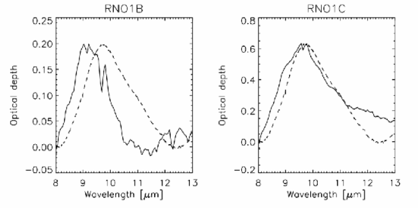
Figure 5: Comparison of the optical depth of the 10$\,\mu$m absorption feature with a typical ISM absorption feature. The solid lines show the optical depth observed towards the RNO complex while the dashed lines represent the (scaled) optical depth towards the galactic center (Kemper et al., 2004). The absorption in the RNO region can not be solely caused by pure ISM silicate grains as both absorption features seem to be slightly shifted towards shorter wavelengths. Furthermore, while the spectrum close to RNO 1C shows additional absorption longwards of 11$\,\mu$m (possibly blended with H₂O ice at 13$\,\mu$m), the feature close to RNO 1B is too narrow and an additional emission feature might contribute longwards of $\sim$10.5$\,\mu$m.

At 6$\,\mu$m both spectra show clear water ice absorption bands. At slightly longer wavelength ($\sim$6.85$\,\mu$m) additional absorption possibly arising from CH₃OH ice is present (van Dishoeck, 2004). The 10$\,\mu$m silicate band is also seen in absorption in both spectra (stronger close to RNO 1C), although the shape of the feature differs from the absorption feature caused by typical interstellar medium silicate grains. To analyze the differences in more detail we fitted a continuum to the 10$\,\mu$m region of the spectra and computed the optical depth (Fig 5). In both cases the peak of the absorption is slightly shifted towards shorter wavelengths indicating a non-ISM like dust composition. Additional absorption (RNO 1C) or possibly additional dust emission on top of the absorption feature (RNO 1B) is seen at longer wavelengths. At 15.2$\,\mu$m CO₂ ice is creating a prominent absorption band and at $\sim$18$\,\mu$m additional silicate absorption seems to be present. All these features indicate the existence of a dense dusty and icy environment in which the two FUORs are embedded. A further analysis of these features also for a larger sample of FUORs will be presented in an upcoming paper (Quanz et al. in preparation).

3.2.2 Pure rotational H₂ emission

In addition to the ice and silicate features, H₂ emission lines from purely rotational quadrupole transitions are present in both spectra (Fig. 4). While in the spectrum close to RNO 1B all transitions from S(1) to S(7) can be identified, the spectrum close to RNO 1C shows only the lines from S(1) to S(5). This can be explained with the higher continuum flux close to the S(6) and S(7) line in the latter spectrum and with apparently lower excitation temperatures (see below). The lowest transition S(0) near 28.22$\,\mu$m is not detected in either spectrum. This is due to the strongly rising continuum at longer wavelengths. Here, the spectral slit contained flux from both RNO objects and also from the deeply embedded IRAS source so that the continuum emission and the related flux errors completely dominate a possible weak emission line. A detailed analysis is provided in the appendix.

Keeping in mind the existence of a molecular outflow that is powered by IRAS 00338+6312 and directly oriented in the direction of RNO 1C and RNO 1B (e.g., Xu et al., 2006), the detection of H₂ emission lines in both spectra hints towards shock induced emission related to the outflow. The spectra consequently bear information about the circumstellar material close to RNO 1B/1C and about the outflow coming from the IRAS source. Since we observe H₂ lines even in the 10$\,\mu$m silicate absorption bands the outflow appears to lie in front of the dusty environment as otherwise the high extinction (A${}_{V}=9.2$ mag and A${}_{V}\approx 12.0$ mag for RNO 1B and RNO1C, respectively, Staude & Neckel, 1991) would have prevented a detection. The measurement of the relative strengths of multiple H₂ lines allows an analysis of the physical conditions of the shocked material. For this we assume local thermal equilibrium (LTE) and optically thin line emission which is supported by the low Einstein coefficients of the involved quadrupole transitions (Table 3). Following Parmar et al. (1991) the column density of an upper energy level $N_{u}(J)$ is then given by

$$N_{u}(J)=\frac{4\pi}{e^{-\tau}}\frac{I(J)}{A_{ul}\,\Delta E_{ul}}\;\rm{cm^{-2}}$$ (1)

where $I(J)$ denotes the observed line intensity in erg s^-1 cm^-2 sr^-1, $\Delta E_{ul}$ is the energy difference of the two states involved in the transition, $A_{ul}$ is the Einstein coefficient for the transition and $\tau$ is the optical depth at the observed wavelength. In Fig. 6 we show Gaussian fits to the observed emission lines in the spectrum close to RNO 1B and Fig. 7 presents corresponding fits to the lines detected close RNO 1C. Before fitting the emission lines we subtracted the underlying continuum which was fitted with a second order polynomial. The finally derived integrated line fluxes and column densities are shown in Table 3. We corrected the line fluxes for extinction effects using the results of Mathis (1990) and assuming $A_{V}=3.55$ mag. This value represents the extinction found by Staude & Neckel (1991) towards the nearby star RNO 1 and should be a better estimate for the line-of-sight extinction than the above mentioned extinction values towards RNO 1B and RNO 1C. In any case the influence of the extinction on the derived shock temperatures and column densities (see below) is negligible. The 1–sigma errors in the line flux, the line intensity and the column density (Table 3) were derived from generating 500 spectra where we added a Gaussian noise to each measured flux point based on the initial individual 1–sigma uncertainty. From these spectra we computed the mean values and related errors of the listed parameters. Especially at the short wavelength end it shows that not all lines were detected with a 3–sigma confidence level. However, since most lines were convincingly measured we decided to keep also the tentative detections in our analyses.

Since we assume LTE the rotational energy levels shall be populated following Boltzmann statistics with a unique temperature for several lines. The involved temperatures $T_{\rm{rot}}$ of the shocked material can be derived from a so–called ”rotational diagram”. By using the results from Eq. 1, plotting the logarithm of $N_{u}(J)/(g_{s}g_{J})$ against $E_{J}/k$ (i.e. the formal temperature corresponding to the absolute upper energy level of the respective rotational transition) and fitting a straight line to the data one finds that the slope of the straight line is proportional to $-1/T_{\rm{rot}}$. Here, $g_{s}$ denotes the spin degeneracy of each energy level (1 for even J, 3 for odd J) and $g_{J}=2J+1$ is the rotational degeneracy. These numbers assume that the ortho–to–para ratio of the involved hydrogen is close to its LTE value of 3 at $T_{\rm{rot}}$. A deviation from this LTE assumption (i.e., ortho–to–para $<$ 3) would result in a downwards displacement of the data points with an odd J-number (ortho–H₂) relative to the points with even J-numbers (para–H₂) and thus create a ”zig–zag” pattern in the rotational plot (e.g., Neufeld et al., 2006; Wilgenbus et al., 2000).

In Fig. 8, 9, and 10 we show rotational plots for the measured lines near RNO 1B and RNO 1C. In all plots the errors for the data points denote the 1–sigma uncertainty in the measured column density.

The rotational diagram of RNO 1B in Fig. 8 shows a clear curvature in the data points. This departure from a single straight line is indicative of several temperature components in the shocked material. We thus fitted the data with two superimposed temperature regimes (hot and warm) that rather represent the minimum and maximum of the involved temperatures than any distinct intermediate value. The dash-dotted line fits the high energy regime and represents the hot component with a temperature of 2991$\pm$596 K. The dotted line corresponds to a temperature of 1071$\pm$121 K designating the warm component. The uncertainties in the temperature denote the 1–sigma confidence level of the fits. As the derived temperature is extremely sensitive to the slope of the fitted straight line the corresponding errors are rather large.

In addition to the temperatures one can also derive the total H₂ column density of the observed shock within the given aperture. From the y-intersects of the fits we estimate the hot component to have $N^{\rm{hot}}_{\rm{1B}}$(H₂)$\approx 1.2\times 10^{17}\;\rm{cm^{-2}}$ and for the warm component we find $N^{\rm{warm}}_{\rm{1B}}$(H₂)$\approx 5.6\times 10^{18}\;\rm{cm^{-2}}$.

For the column densities derived from the spectrum close to RNO 1C we plotted two rotational diagrams shown in Fig. 9 and 10. First, we fitted the data with a single temperature component of 1754$\pm$321 K. However, the shocked material is apparently not in LTE as the data points with odd and even J-numbers are difficult to fit simultaneously with a straight line or a curve. As mentioned above this displacement is indicative of a departure from the LTE ortho–to–para ratio of 3. Fig. 10 shows the same data if one assumes an ortho–to–para ratio of 1. Now, a two component fit, similar to that in Fig. 8, is possible. For the hot component we derive a temperature of 2339$\pm$468 K, while the warm component is significantly colder with 466$\pm$264 K. The total H₂ column densities amount to $N^{\rm{hot}}_{\rm{1C}}$(H₂)$\approx 5.5\times 10^{17}\;\rm{cm^{-2}}$ and $N^{\rm{warm}}_{\rm{1C}}$(H₂)$\approx 9.7\times 10^{19}\;\rm{cm^{-2}}$, respectively.

Table 4 summarizes the temperatures and total column densities of the different components for both spectra.

4 Discussion

The IRAC images reveal for the first time the embedded MIR point source associated with IRAS 00338+6312. However, already Weintraub & Kastner (1993) concluded from polarimetric observations that an additional source should be present close to the IRAS point source position. Furthermore, many authors analyzing the bipolar outflow related to this region concluded that a deeply embedded object was most likely the driving source (Yang et al., 1995; Xu et al., 2006; Weintraub & Kastner, 1993) instead of one of the RNO objects (McMuldroch et al., 1995). Previous ground based MIR observations (Polomski et al., 2005) were possibly not sensitive enough to detect IRAS 00338+6312.

The observed properties of IRAS 00338+6312 convincingly classify the object as a young protostar and support the idea that it is indeed driving the molecular outflow. From their CO measurements Xu et al. (2006) derived a total mass for this bipolar outflow of 1.4 M_☉, indicating that IRAS 00338+6312 is an intermediate–mass protostar. The detection of the IRAS source solves also the problem that up to now the SEDs of RNO 1B and RNO 1C were unusually steep longward of 25$\,\mu$m for FUOR objects (Weintraub & Kastner, 1993). The images presented here have sufficient sensitivity and spatial resolution to show that the newly revealed source associated with IRAS 00338+6312 is most probably responsible for this flux excess.

In addition to the IRAS object Weintraub & Kastner (1993) also suspected another embedded source which we identify with RNO 1G. Furthermore, the detection of RNO 1F (Weintraub et al., 1996), which was initially assumed to be a density enhancement rather than an independent self-luminous source (Weintraub & Kastner, 1993), is confirmed with our IRAC images. Only RNO 1D, which was thought to be located between RNO 1B and RNO 1C (Staude & Neckel, 1991), does not show up in our images. This source was, however, also not detected by Weintraub & Kastner (1993) and only tentatively seen in the data from Weintraub et al. (1996).

It is not clear whether all detected objects are physically confined to the RNO 1B/1C region. Especially the membership of the newly discovered objects RNO1 IRAC1, RNO1 IRAC2, and RNO1 IRAC3 needs to be confirmed. However, the IRAC observations suggest that RNO 1B and RNO 1C belong to a small cluster of (partly very) young objects. To our knowledge, although some FUORs are known or suspected to be in binary or multiple systems (e.g., Reipurth & Aspin, 2004), the existence of FUORs in a cluster-like environment is a so far unique finding. Only the FUOR candidate V1184 Tau (CB34) belongs also to a small cluster (Khanzadyan et al., 2002) but its classification as FUOR is far less certain than for the RNO objects (Yun et al., 1997). In any case the still deeply embedded protostars in the close vicinity of RNO 1B/1C put strong constraints on the age of the objects if one assumes coeval evolution.

The magnitudes we derive for the two FUOR objects at 3.6$\,\mu$m can be compared to previous ground based measurements at 3.8$\,\mu$m by Kenyon et al. (1993) and Polomski et al. (2005). However, one certainly has to keep in mind that the IRAC filter is not only different in terms of central wavelength but also the spectral width differs from that of the ground based instruments. While Kenyon et al. (1993) found $L_{3.8\,\mu\rm m}=6.36$ mag and $L_{3.8\,\mu\rm m}=6.5\,$mag for RNO 1B and RNO 1C, respectively, Polomski et al. (2005) observed RNO 1C to be slightly brighter than RNO 1B ($L_{3.8\,\mu\rm m}=6.27\,$mag vs. $L_{3.8\,\mu\rm m}=6.42\,$mag). Also in our measurements RNO 1C seems to be the brighter component. However, both objects appear to be fainter in our observations compared to Polomski et al. (2005). Apart from the differences in the filter properties intrinsic variations in the luminosity of the FUORs and/or changing local extinction effects can account for the apparent variability in these objects.

The detection of H₂ rotational line emission can in general be attributed to collisional excitation from C- or J-type shocks (e.g., Draine & McKee, 1993; Moro-Martín et al., 2001). C-type shocks are magnetic and less violent towards molecules in comparison to the mostly hydrodynamic J-type shocks that can dissociate H₂ molecules even at lower shock velocities. From our rotational diagrams we derived shock temperatures that are similar to those found in the outflow from Cepheus A (Froebrich et al., 2002). These authors could fit a two component C-shock model to their data and derived shock velocities between 25 and 30 km s^-1 for a cold and a hot component, respectively. By comparing our results directly to theoretical shock models we find that the C-shock Model 1 from Timmermann (1998) can explain both the hot and warm component in the spectrum close to RNO 1B. Considering our derived temperatures as an upper and lower limit for the shocked material, shock velocities between 15 and 30 km s^-1 are required. However, Model 1 of Timmermann (1998) predicts on ortho–to–para ratio of $\approx$2 at the low velocity/low temperature limit which is not directly evident from our observations. More recent models by Wilgenbus et al. (2000) predict lower shock temperatures in C-type shocks for the same shock velocities in comparison to Timmermann (1998). Following their models, our hot component in Fig.8 requires velocities exceeding 40 km s^-1. Slightly slower velocities ($\approx$35 km s^-1) are already needed to explain the hot temperature component in the shock close to RNO 1C (Fig. 10). The warm component in this diagram represents shock velocities between 15 km s^-1 and 20 km s^-1. Although it is clear that some uncertainties between the observations and theory still remain, C-type shocks seem to provide a solid explanation for the observed shock temperatures.

The measurement of an ortho–to–para ratio smaller than 3 in Fig. 10 implies that despite the high temperatures the gas has not yet reached equilibrium between the ortho and para states. Thus, the observed ratio is the legacy of the temperature history of the gas (see, e.g., Neufeld et al., 1998, 2006) and transient heating by a recently passing shock wave already caused higher temperatures. As the corresponding region on the sky lies closer to the IRAS source than the region probed in Fig. 8, the observations suggest that we see the signatures of at least two shock waves: The first shock wave is probed close to RNO 1B (Fig. 8) where we observe several temperature components that have apparently reached their equilibrium state. A more recent shock wave is seen close to RNO 1C (Fig. 10) where the ratio of the line column densities hints also towards high shock velocities and temperatures but the gas is not yet in thermal equilibrium.

5 Conclusions and Future Prospects

Our conclusions can be summarized as follows:

• We detected and resolve for the first time the MIR point source associated with IRAS 00338+6312 which appears to be an embedded intermediate–mass protostar driving the known molecular outflow in the RNO 1B/1C region.

• The detection of additional (partly previously unknown) point sources suggests that the FUOR objects RNO 1B/1C belong to a young small stellar cluster. To our knowledge, RNO 1B/1C are the only well–studied and confirmed FUORs that apparently belong to a cluster–like environment.

• All but two objects were detected in all four IRAC bands and their colors are consistent with Class 0/I-II objects. The two objects that were not detected at 3.6$\,\mu$m (including IRAS 00338+6312) are still very deeply embedded protostars.

• Having apparently extremely young objects in the direct vicinity of the FUORs confirms the suspected young age for this type of objects although their MIR colors are consistent with Class II objects.

• The two MIR spectra of the region bear clear signs of a dense icy and dusty circumstellar environment as solid state features are seen in absorption.

• The spectra show also H₂ emission lines from purely rotational transitions. We presume that these lines arise from shocked material within the molecular outflow. The derived shock temperatures and velocities are in agreement with C-type shock models.

• The observations of the H₂ lines suggest that the outflow lies in front of RNO 1B/1C as otherwise the high optical depth towards these objects would have prevented the detection.

• While in one spectrum the gas probed by the H₂ line emission seems to be in LTE, the other spectrum shows a deviation from the expected LTE ortho–to–para H₂ ratio. This indicates the presence of at least two shock waves, the most recent one responsible for the non–LTE line ratios.

The results presented here advantageously combine space-based MIR imaging and spectroscopy. While the images give insights into the photometric properties of several young embedded objects and also FU Orionis type stars the spectra provide information on the dusty and icy circumstellar environment of the young cluster as well as on shocked gas within a molecular outflow. In this context the existence of FUORs in a cluster–like environment needs to be pointed out. It is still debated whether all young low–mass stars undergo an FUOR phase or whether these objects form a special sub–group of YSOs (e.g., Hartmann & Kenyon, 1996). Our results suggests that the FUOR phenomenon occurs also in young (small) stellar clusters making it thus possibly more common than so far expected. In addition, the co–existence of FUORs and very young protostars in the same environment strengthens the idea that the FUOR–phase of YSOs is linked to the early stages of the star formation process.

Possible future investigations of the RNO 1B/1C region should address whether the observed objects do indeed belong to the same region and whether all of them are young stars. Furthermore, a detailed study of the shocked material including high–resolution narrow band imaging and spectroscopic mapping (e.g., with Spitzer IRS) will provide deeper insights into its extension, physical conditions, and its relation to the molecular outflow. A complete analysis of the ice and dust features in the observed spectra is currently underway and will be presented in an upcoming paper (Quanz et al. in preparation).

Appendix A The non-detection of the 28.22$\,\mu$m emission line

In the following we analyze whether the non-detection of the 28.22$\,\mu$m in either spectrum is in agreement with the models. The two component models in Fig. 8 and  10 can be used to predict the column densities of the S(0) emission line. One expects

$$\rm{log}\frac{N_{\rm{S(0)}}}{g_{j}g_{s}}[\rm{cm}^{-2}]\approx 18.3\,\rm{cm}^{-2}$$

$$\rm{log}\frac{N_{\rm{S(0)}}}{g_{j}g_{s}}[\rm{cm}^{-2}]\approx 18.8\,\rm{cm}^{-2}$$

for the spectrum close to RNO 1B and RNO 1C, respectively. With $g_{s}$=1 and $g_{j}$=5 and applying Eq. (1) the following line intensities are derived:

$$\rm I(2)_{\rm{1B}}\approx 1.64\cdot 10^{-6}\,\rm{erg\,s^{-1}\,cm^{-2}\,sr^{-1}}$$

$$\rm I(2)_{\rm{1C}}\approx 5.20\cdot 10^{-6}\,\rm{erg\,s^{-1}\,cm^{-2}\,sr^{-1}}$$

The $A$-coefficient for the transition is $2.94\cdot 10^{-11}$s^-1 (Wolniewicz et al., 1998).

Taking into account the aperture size for the long wavelength high–resolution module of the spectrograph of 247.53 arcsec² ($\approx 5.82\cdot 10^{-9}\,\rm{sr}$) the predicted integrated line fluxes amount to:

$$\rm F_{\rm{1B}}\approx 9.57\cdot 10^{-22}\,\rm W\,\rm{cm}^{-2}$$

$$\rm F_{\rm{1C}}\approx 3.02\cdot 10^{-21}\,\rm W\,\rm{cm}^{-2}$$

To estimate the peak of the 28.22$\,\mu$m line in Jansky we assume that the spectral resolution in the high–resolution modules is constant and that the FWHM of the S(0) line can be extrapolated from the FWHM of the S(1) line at 17.03$\,\mu$m. Since we fit a Gaussian profile to the emission lines and we want to derive the peak flux of this Gaussian, we also have to take into account the relation between the FWHM we measure for the line and the $\sigma$ of the profile. This relation is FWHW=$\sqrt{8\,\rm{ln}2}\cdot\sigma$. With the expected FWHM of

$$\Delta\nu_{\rm{1B}}\approx 2.84\cdot 10^{10}\,\rm{Hz}$$

$$\Delta\nu_{\rm{1C}}\approx 2.12\cdot 10^{10}\,\rm{Hz}$$

we find thus corresponding peak fluxes of:

$$\rm F^{\rm{peak}}_{\rm{1B}}\approx 0.034\,\rm{Jy}$$

$$\rm F^{\rm{peak}}_{\rm{1B}}\approx 0.152\,\rm{Jy}$$

These values have to be compared to the measured uncertainties in the spectra. The mean 1–$\sigma$ level in the spectral range between 28.0 and 28.4$\,\mu$m is, however,

$$\bar{\sigma}_{\rm{1B}}=0.055$$

$$\bar{\sigma}_{\rm{1C}}=0.082$$

so that even in the more favorable case of RNO 1C the emission line is not expected to be detected with a confidence level greater than $\approx$1.8$\,\sigma$.

Table 1: Journal of observations.

Instrument	RA (2000)	DEC (2000)	AOR Key	Filter or Module	Ramp duration /	Frame Time /	Date
					# of Cycles	# of Frames /
						Dither Positions
Spitzer IRAC	00:36:45.8	+63:28:56	5027072	3.6, 4.5, 5.8, 8.0$\,\mu$m	-	0.4 / 1 / 4	2003-12-20
Spitzer IRS	00:36:46.34	+63:28:53.76	6586624	Low Resolution	6 sec / 3	-	2004-01-07
	00:36:46.89	+63:28:58.44
Spitzer IRS	00:36:46.34	+63:28:53.76	6586624	High Resolution	6 sec / 5	-	2004-01-07
	00:36:46.89	+63:28:58.44

Table 2: Apparent brightness at different wavelengths for objects that were detected in at least three IRAC bands. The coordinates are measured in the 3.6$\,\mu$m image. Only the positions of the IRAS source and RNO 1G were measured in the 4.5$\,\mu$m exposure.

No.	Object name	RA (J2000)	DEC (J2000)	3.6$\,\mu$m	4.5$\,\mu$m	5.8$\,\mu$m	8.0$\,\mu$m
				[mag]	[mag]	[mag]	[mag]
1	RNO 1B	00:36:46.05	+63:28:53.29	7.16$\pm$0.13	6.67$\pm$0.06	5.76$\pm$0.12	5.01$\pm$0.09
2	RNO 1C	00:36:46.65	+63:28:57.90	6.56$\pm$0.01	6.04$\pm$0.01	5.58$\pm$0.01	4.61$\pm$0.02
3	RNO 1F	00:36:45.74	+63:29:04.09	10.28$\pm$0.09	9.46$\pm$0.08	8.58$\pm$0.05	8.20$\pm$0.03
4	RNO 1G	00:36:47.14	+63:28:49.95	-	10.33$\pm$0.06	8.74$\pm$0.04	8.05$\pm$0.07
5	IRAS 00338+6312	00:36:47.34	+63:29:01.61	-	9.05$\pm$0.07	7.19$\pm$0.05	6.72$\pm$0.03
6	RNO1 IRAC1	00:36:48.44	+63:28:39.98	13.72$\pm$0.15	11.82$\pm$0.14	10.93$\pm$0.20	9.65$\pm$0.04
7	RNO1 IRAC2	00:36:47.90	+63:28:36.30	12.00$\pm$0.08	10.86$\pm$0.10	10.86$\pm$0.16	9.82$\pm$0.14
8	RNO1 IRAC3	00:36:47.85	+63:28:41.23	13.07$\pm$0.10	11.78$\pm$0.08	10.74$\pm$ 0.10	9.74$\pm$0.05

Table 3: Properties of the observed Hydrogen emission lines close to RNO 1B (upper part) and RNO 1C (lower part). The numbers in parentheses denote powers of ten. The 12.28$\,\mu$m emission line close to RNO 1B was measured in the low– and high–resolution part of the spectrograph. See text for discussion about the apparent flux difference between the two measurements.

Transition	Wavelength	Energy	$A$-Coefficient	Beam Size	Line Flux	Line Intensity	Column Density
	[$\,\mu$m]	EJ/k [K]	[s-1]	[arcsec2]	[W cm-2]	[erg cm-2 s-1 sr-1]	[cm-2]
H2 lines close to RNO 1B
S(1) J=3-1	17.0348	1015.08	4.76(-10)	53.11	7.91(-21)$\pm$3.8(-22)	6.34(-5)$\pm$3.0(-6)	1.44(19)$\pm$6.8(17)
S(2) J=4-2	12.2786	1681.63	2.75(-9)	53.11	1.33(-20)$\pm$5.2(-22)	1.06(-4)$\pm$4.1(-6)	3.00(18)$\pm$1.2(17)
				39.96	6.75(-21)$\pm$1.2(-21)	7.18(-5)$\pm$1.3(-5)	2.03(18)$\pm$3.7(17)
S(3) J=5-3	9.6649	2503.73	9.83(-9)	39.96	2.00(-20)$\pm$2.7(-21)	2.13(-4)$\pm$2.9(-5)	1.33(18)$\pm$1.8(17)
S(4) J=6-4	8.0251	3474.48	2.64(-8)	39.96	9.12(-21)$\pm$1.9(-21)	9.71(-5)$\pm$2.1(-5)	1.87(17)$\pm$4.0(16)
S(5) J=7-5	6.9095	4585.94	5.88(-8)	39.96	2.13(-20)$\pm$2.6(-21)	2.26(-4)$\pm$2.8(-5)	1.68(17)$\pm$2.1(16)
S(6) J=8-6	6.1086	5829.66	1.14(-7)	39.96	7.04(-21)$\pm$1.3(-21)	7.50(-5)$\pm$1.4(-5)	2.54(16)$\pm$4.8(15)
S(7) J=9-7	5.5112	7196.20	2.00(-7)	39.96	1.32(-20)$\pm$6.1(-21)	1.41(-4)$\pm$6.5(-5)	2.46(16)$\pm$1.1(16)
H2 lines close to RNO 1C
S(1) J=3-1	17.0348	1015.08	4.76(-10)	53.11	3.26(-21)$\pm$2.7(-22)	2.61(-5)$\pm$2.1(-6)	5.92(18)$\pm$4.8(17)
S(2) J=4-2	12.2786	1681.63	2.75(-9)	53.11	5.17(-21)$\pm$7.7(-22)	4.14(-5)$\pm$6.2(-6)	1.17(18)$\pm$1.7(17)
S(3) J=5-3	9.6649	2503.73	9.83(-9)	39.96	7.52(-21)$\pm$2.0(-21)	8.00(-5)$\pm$2.1(-5)	4.98(17)$\pm$1.3(17)
S(4) J=6-4	8.0251	3474.48	2.64(-8)	39.96	1.34(-20)$\pm$4.1(-21)	1.43(-4)$\pm$4.4(-5)	2.74(17)$\pm$8.5(16)
S(5) J=7-5	6.9095	4585.94	5.88(-8)	39.96	1.10(-20)$\pm$3.3(-21)	1.17(-4)$\pm$3.5(-5)	8.69(16)$\pm$2.6(16)

Table 4: Upper and lower limits on the temperatures, and the total H₂ column densities of the observed shocked components. For the data derived close to RNO 1C the results from the two component fit and the single component fit with different ortho–to–para ratios are given.

Component	T [K]	log10 N(H2) [cm-2]
RNO 1B
Hot	2991$\pm$596	17.09$\pm$0.36
Warm	1071$\pm$121	18.75$\pm$0.09
RNO 1C
Hot	2339$\pm$468	17.74$\pm$0.31
Warm	466$\pm$264	19.99$\pm$1.17
Single	1754$\pm$321	17.98$\pm$0.31

Figure 3: IRAC color-color plots for the objects listed in Table 2. The dashed boxes indicate the regions corresponding to Class II objects in Hartmann et al. (2005). The dashed-dotted region in the right plot defines the position of Class 0/I sources in Hartmann et al. (2005). In the left plot the Class 0/I objects from Hartmann et al. (2005) have the same [5.8]-[8.0] colors as the Class II objects but redder [3.6]-[4.5] colors. Thus, they lie ”above” the dashed box. The reddening vectors correspond to $A_{V}=30$ mag and are based on a Vega-like spectrum and the reddening law given by Mathis (1990).

.

.

Figure 6: Gaussian fits to the H₂ lines in the spectrum close to RNO 1B after continuum subtraction. The line at 12.28$\,\mu$m shown here was measured in the low–resolution spectrum. Table 3, however, contains the flux of this line measured in both, the low– and high–resolution part of the spectrum. The line at 6.11$\,\mu$m is blended with the ice feature in this region.

Figure 7: Same as Fig. 6 but for the spectrum close to RNO 1C. Here, the 12.28$\,\mu$m line was only detected in the high–resolution spectrum.

Figure 8: Rotational diagram of the H₂ lines shown in Fig. 6. The data are well constrained by the superposition of a hot and a warm component providing an upper and a lower limit for the temperature range of the shocked gas. The diamond at $\approx$1682 K corresponds to the 12.28$\,\mu$m line measured in the high–resolution module. The observed line flux, and hence the derived column density, is slightly higher than that in the low–resolution spectrum. For the fit, however, the low–resolution data point was used as all other higher energy data points were also obtained with the low–resolution spectrograph and uncertainties related to the different apertures and their orientations for the high– and low–resolution modules are thus minimized.

Figure 9: Rotational diagram of the H₂ lines shown in Fig. 6. The apparent zig-zag pattern is indicative of an ortho–to–para ratio smaller than 3.

Figure 10: Same as Fig. 9 but now for an assumed ortho–to–para ratio of 1. A two component fit similar to that in Fig. 8 is now possible.

References

- Anglada et al. (1994) Anglada, G., Rodriguez, L. F., Girart, J. M., Estalella, R., & Torrelles, J. M. 1994, ApJ, 420, L91
- Draine & McKee (1993) Draine, B. T. & McKee, C. F. 1993, ARA&A, 31, 373
- Fiebig (1995) Fiebig, D. 1995, A&A, 298, 207
- Froebrich et al. (2002) Froebrich, D., Smith, M. D., & Eislöffel, J. 2002, A&A, 385, 239
- Hartmann & Kenyon (1996) Hartmann, L. & Kenyon, S. J. 1996, ARA&A, 34, 207
- Hartmann et al. (2005) Hartmann, L., Megeath, S. T., Allen, L., Luhman, K., Calvet, N., D’Alessio, P., Franco-Hernandez, R., & Fazio, G. 2005, ApJ, 629, 881
- Higdon et al. (2004) Higdon, S. J. U., Devost, D., Higdon, J. L., Brandl, B. R., Houck, J. R., Hall, P., Barry, D., Charmandaris, V., Smith, J. D. T., Sloan, G. C., & Green, J. 2004, PASP, 116, 975
- Jennings et al. (1987) Jennings, D. E., Weber, A., & Brault, J. W. 1987, Journal of Molecular Spectroscopy, 126, 19
- Kemper et al. (2004) Kemper, F., Vriend, W. J., & Tielens, A. G. G. M. 2004, ApJ, 609, 826
- Kenyon et al. (1993) Kenyon, S. J., Hartmann, L., Gomez, M., Carr, J. S., & Tokunaga, A. 1993, AJ, 105, 1505
- Khanzadyan et al. (2002) Khanzadyan, T., Smith, M. D., Gredel, R., Stanke, T., & Davis, C. J. 2002, A&A, 383, 502
- Mathis (1990) Mathis, J. S. 1990, ARA&A, 28, 37
- McMuldroch et al. (1995) McMuldroch, S., Blake, G. A., & Sargent, A. I. 1995, AJ, 110, 354
- Moro-Martín et al. (2001) Moro-Martín, A., Noriega-Crespo, A., Molinari, S., Testi, L., Cernicharo, J., & Sargent, A. 2001, ApJ, 555, 146
- Neufeld et al. (1998) Neufeld, D. A., Melnick, G. J., & Harwit, M. 1998, ApJ, 506, L75
- Neufeld et al. (2006) Neufeld, D. A., Melnick, G. J., Sonnentrucker, P., Bergin, E. A., Green, J. D., Kim, K. H., Watson, D. M., Forrest, W. J., & Pipher, J. L. 2006, ApJ, 649, 816
- Parmar et al. (1991) Parmar, P. S., Lacy, J. H., & Achtermann, J. M. 1991, ApJ, 372, L25
- Persi et al. (1988) Persi, P., Ferrari-Toniolo, M., Busso, M., Robberto, M., Scaltriti, F., & Silvestro, G. 1988, AJ, 95, 1167
- Polomski et al. (2005) Polomski, E. F., Woodward, C. E., Holmes, E. K., Butner, H. M., Lynch, D. K., Russell, R. W., Sitko, M. L., Wooden, D. H., Telesco, C. M., & Piña, R. 2005, AJ, 129, 1035
- Reipurth & Aspin (2004) Reipurth, B. & Aspin, C. 2004, ApJ, 608, L65
- Snell et al. (1990) Snell, R. L., Dickman, R. L., & Huang, Y.-L. 1990, ApJ, 352, 139
- Staude & Neckel (1991) Staude, H. J. & Neckel, T. 1991, A&A, 244, L13
- Timmermann (1998) Timmermann, R. 1998, ApJ, 498, 246
- van Dishoeck (2004) van Dishoeck, E. F. 2004, ARA&A, 42, 119
- Weintraub & Kastner (1993) Weintraub, D. A. & Kastner, J. 1993, ApJ, 411, 767
- Weintraub et al. (1996) Weintraub, D. A., Kastner, J. H., Gatley, I., & Merrill, K. M. 1996, ApJ, 468, L45+
- Wilgenbus et al. (2000) Wilgenbus, D., Cabrit, S., Pineau des Forêts, G., & Flower, D. R. 2000, A&A, 356, 1010
- Wolniewicz et al. (1998) Wolniewicz, L., Simbotin, I., & Dalgarno, A. 1998, ApJS, 115, 293
- Xu et al. (2006) Xu, Y., Shen, Z.-Q., Yang, J., Zheng, X. W., Miyazaki, A., Sunada, K., Ma, H. J., Li, J. J., Sun, J. X., & Pei, C. C. 2006, AJ, 132, 20
- Yang et al. (1995) Yang, J., Ohashi, N., & Fukui, Y. 1995, ApJ, 455, 175
- Yang et al. (1991) Yang, J., Umemoto, T., Iwata, T., & Fukui, Y. 1991, ApJ, 373, 137
- Yun et al. (1997) Yun, J. L., Moreira, M. C., Alves, J. F., & Storm, J. 1997, A&A, 320, 167