Thermal instability in X-ray photoionized media
in Active Galactic Nuclei:

Abstract

Context. A photoionized gas in thermal equilibrium can display a thermal instability, with three or more solutions in the multi-branch region of the S-shape curve giving the temperature versus the radiation-to-gas-pressure ratio. Many studies have been devoted to this curve and to its dependence on different parameters, always in the optically thin case.

Aims. The purpose of our study is the thermal instability in optically thick, stratified media, in total pressure equilibrium. We are also interested in comparing photoionization models issued from the hot and cold stable solutions, with the currently used models computed with an approximate, intermediate solution.

Methods. We have developped a new algorithm to select the hot/cold stable solution, and thereof to compute a fully consistent photoionization model. We have implemented it in the TITAN code and computed a set of models encompassing the range of conditions valid for the Warm Absorber in Active Galactic Nuclei.

Results. We have demonstrated that the thermal instability problem is quite different in thin or thick media. Models computed with the hot/cold stable solutions, or with an intermediate solution, differ all along the gas slab, with the spectral distribution changing as the radiation progresses inside the ionized gas. These effects depend on the thickess of the medium and on its ionization.

Conclusions. This has observational implications in the emitted/absorbed spectra, ionization states, and variability. However impossible to know what solution the plasma will adopt when attaining the multi-solutions regime, we expect the emitted/absorbed spectrum to be intermediate between those resulting from pure cold and hot models; such a phase-mixed medium can be well reproduced by intermediate solution models. Large spectral fluctuations corresponding to the onset of a cold/hot solution could be observed in timescales of the order of the dynamical time. A strong turbulence implying supersonic velocities should permanently exist in the multi-branch region of thick, stratified, pressure equilibrium media.

1 Introduction

It is well known that a photoionized gas in thermal equilibrium, i.e. a gas where the radiative heating is balanced by radiative cooling, can display a thermal instability (e.g., Krolik, Tarter & McKee 1981). The phenomenon manifests itself in the S-shape of the net cooling function or, which is equivalent, through the curve giving the temperature versus the radiation-to-gas-pressure ratio. Such an S-shape curve allows for the co-existence of gas at different temperatures and densities for the same pressure ratio.

For a given value of the radiation-to-gas-pressure ratio, the gas can then be in three (or even more) states of thermal equilibrium, which depend on the Spectral Energy Distribution (SED) of the ionizing spectrum, on the abundances, and on other physical parameters affecting the heating and the cooling. One of these states is thermally unstable, as it does not satisfy the stability criterium to isobaric perturbations (Field 1965):

$$(\frac{\partial{\cal L}}{\partial T})_{P_{\rm gas}}>0,$$ (1)

where ${\cal L}$ is the net cooling function, $T$ is the temperature, and $P_{\rm gas}$ is the gas pressure. The two other states for which the derivative of ${\cal L}$ is positive, are stable. Such thermal instability is, for instance, at the origin of the two-phase model for the interstellar medium, where cold ($T\lesssim 300$ K) neutral atomic and molecular clouds are embedded in a warm ($T\sim 10^{4}$ K) intercloud medium (Field, Goldsmith & Habing 1969).

1.1 Optically thin media

Krolik et al. (1981) studied the thermal instability in the context of Active Galactic Nuclei (AGN), for optically thin, X-ray illuminated gas. In such media, the radiation pressure keeps a constant value, and the energy balance equation solution depends on the gas pressure only. When the gas pressure is small compared to the radiation pressure, there is a unique, stable, “hot” solution, where both the heating and the cooling are dominated by Compton processes (Compton heating, inverse Compton cooling). As the gas pressure increases, atomic processes (photoionization heating, line and continuum cooling) become important, and multiple solutions arise. The harder the spectrum, the more extended is the region encompassed by the multiple solutions. Then, above a given gas pressure, again a unique, but this time “cold” solution, arises. Krolik et al. showed that such multiple solutions may lead to the existence of a two-phase medium consisting of a hot, dilute gas confining denser, cooler clumps, which they identified as the Broad Line Region in AGN.

To better address the thermal instability issue, these authors introduced the ionization parameter $\Xi$ (dimensionless), defined as

$$\Xi=\frac{F_{\rm ion}}{n\,kT\/c}\ ,$$ (2)

where $F_{\rm ion}$ is the incident ionizing flux between 1 and $10^{3}$ Rydberg, $n$ is the total numerical density, and $T$ the gas temperature. In a fully ionized gas, the radiation-to-gas-pressure ratio, $P_{\rm rad}/P_{\rm gas}$, is about equal to $\Xi/2.3$. The so-called S-shape curve is thus, actually, the curve giving $T$ versus $\Xi$. Krolik et al. showed that the multi-branch region of this curve (or, which is equivalent, the multi-solutions regime) corresponds to a range of $\Xi$ between 1 and 10 for a typical AGN spectrum.

Since then, many studies have been devoted to the S-shape curve and to its dependence on the incident ionizing spectrum and on the abundances, but always in the optically thin case. The purpose of our study is different from previous works, as we are interested in optically thick media such as the Warm Absorber (WA) in type 1 AGN, the X-ray line-emitting gas in type 2 AGN, or irradiated accretion discs in AGN and X-ray binaries. Our studies may be applied to media in any pressure equilibrium conditions, e.g., constant gas pressure, constant total pressure, or hydrostatic pressure equilibrium.

1.2 Optically thick media

Let us assume a medium in total pressure equilibrium, consisting of a slab of gas with a given density at the illuminated surface. Under such conditions, irradiation by X-rays induces a thermal instability beyond a given layer in the slab. The shape of the radiation spectrum and the radiation pressure itself, depend on the considered position in the gas slab. Near the surface, the radiation spectrum is close to the incident spectrum irradiating the slab (close, yet different, owing to the additional presence of radiation returned by the non-illuminated side of the slab).

If the radiation-to-gas-pressure ratio is sufficiently large, the equilibrium temperature is high, and these layers are hot, displaying a unique, “hot” solution. Such equilibrium temperature stays almost constant in this region. In deeper layers, two effects take place. First, the radiation spectrum is harder, owing to soft X-ray absorption by the previous layers; it contains only hard X-rays and diffuse ultraviolet radiation created within the slab. As a consequence, the S-shape curve is more pronounced. Second, in the conditions of our models (described in Sec. 3), the radiation flux decreases — and so does the radiation pressure — entraining the gas to enter the multi-solutions regime; the gas has now the choice between two stable solutions, a “hot” and a “cold” one. Finally, as the radiation penetrates still deeper in the slab, it suffers more and more modifications, and we get to a point where there is again a unique, “cold” solution. The corresponding equilibrium temperature remains almost constant again. This phenomenon can occur several times in the slab, according to the spectral distribution of the specific intensity through the medium. Each time the gas-phase changes, adjusting to a colder solution, the temperature profile displays a sharp drop by one order of magnitude or so. In between phase changes, the temperature remains more or less constant.

1.3 Electronic conductivity and alternative methods

One of the questions one may ask at this stage is “which solution to choose when there are two or more stable ones?” The answer depends on the previous history of the medium. A unique equilibrium state could be found if electron conduction was to be included (Begelman & McKee 1990; McKee & Begelman 1990; Różańska 1999). The well-known numerical difficulty linked to the thermal instability could be overcomed using an integral formulation of the criterium giving the equilibrium solution, instead of a differential one (Różańska & Czerny 2000). However, coupling conductivity effects with a complete radiative transfer in photoionization models is a complicated task, and has not yet been performed. Attempts to introduce electonic conduction are presently being undertaken by Chevallier et al. (in preparation).

There are, however, other means to circumvent the problem of multiple stable solutions when dealing with photoionization codes. Two possibilities are discussed here: the first one was used to compute the vertical structure of irradiated accretion discs in hydrostatic equilibrium (e.g., Ko & Kallman 1994). This method consists in keeping the gas pressure constant during the iterations for convergence of the energy balance equation; this procedure is correct, but leads to a situation of thermal instability, as described in the previous sections. Photoionization codes using this computational method (e.g. XSTAR: Kallman & Krolik 1995; Kallman & Bautista 2001) must then choose arbitrarily one of the stable solutions in the multi-branch region. The second possibility is to keep the density constant during the iterations for convergence of the energy balance equation, allowing to obtain the temperature value in the layer; this computational method provides a unique solution, even if it is an approximate one, intermediate between the “cold” and the “hot” solutions present in the multi-branch region. This approach has been used in studies of the vertical structure of accretion discs (Raymond 1993; Shimura, Mineshige & Takahara 1995; Madej & Różańska 2000; Kawaguchi, Shimura & Mineshige 2001; Ballantyne et al. 2001).

Such a computational method is implemented in our photoionization code TITAN, described in the following section. It has been used during the past years, with good results; models computed with the “intermediate” temperature solution have been applied, for instance, to studies of the vertical disc structure with hydrostatic equilibrium (Różańska et al. 2002), and to total pressure equilibrium media (Różańska et al. 2002; Dumont et al. 2002; Różańska et al. 2006; Gonçalves et al. 2006; Chevallier et al. 2006a). Since then, we have implemented a new algorithm in the TITAN code; here, we report on this new addition and its applications. In summary, the new algorithm allows to choose between the “hot” or the “cold” stable solutions in the multi-branch region, and thereof to compute a fully consistent model using the chosen solution. For the first time, it is thus possible to compare models issued from the true stable solutions with the approximate solution model and to estimate the degree of uncertainty of such an “intermediate” solution. Our improved version of the TITAN code will allow to better understand the behavior of both kind of computational schemes and to estimate their influence on the description of the ionized gas structure and on the modelled spectra emitted and absorbed by the medium.

In Sect. 2 we give a brief description of the TITAN code and discuss the different computational methods used in more detail; the models are described in Sect. 3. Section 4 contains a comparative study between the “hot”, “cold”, and “intermediate” solutions. In Sect. 5 we discuss some observational implications, and in Sect. 6 we summarize our conclusions.

2 Computational issues

2.1 The TITAN code

All our models, summarized in Table 1, were computed using the TITAN code. TITAN is a photoionization-transfer code developed by our team to correctly model optically thick (Thomson optical depth up to several tens) ionized media; it can equally be applied to thinner media (Thomson depth $\sim$ 0.001 to 0.1, e.g., Collin et al. 2004; Gonçalves et al. 2006). The code includes all relevant physical processes (e.g., photoionization, radiative and dielectronic recombination, fluorescence and Auger processes, collisional ionization, radiative and collisional excitation/de-excitation, etc.) and all induced processes. It solves the ionization equilibrium of all the ion species of each element, the thermal equilibrium, the statistical equilibrium of all the levels of each ion, and the transfer of both the lines and the continuum. It gives as output the ionization, density, and temperature structures, as well as the reflected, outward, and transmitted spectra. The energy balance is ensured locally with a precision of 0.01%, and globally with a precision of 1%.

Model	$\xi=L/n_{\rm H}R^{2}$	$N_{\rm H}$	Thermal instability
name	(erg cm s-1)	(cm-2)	solution
HI 1_C	10000	2 1023	cold
HI 1_H	10000	2 1023	hot
HI 1_I	10000	2 1023	intermediate
MI 1_C	1000	2 1023	cold
MI 1_H	1000	2 1023	hot
MI 1_I	1000	2 1023	intermediate
MI 2_C	1000	2.5 1023	cold
MI 2_H	1000	2.5 1023	hot
MI 2_I	1000	2.5 1023	intermediate
MI 3_C	1000	3 1023	cold
MI 3_H	1000	3 1023	hot
MI 3_I	1000	3 1023	intermediate
LI 1_C	300	5 1022	cold
LI 1_H	300	5 1022	hot
LI 1_I	300	5 1022	intermediate
LI 2_C	300	8.5 1022	cold
LI 2_H	300	8.5 1022	hot
LI 2_I	300	8.5 1022	intermediate

Table 1: Models computed with TITAN in the framework of this study. In the first column, the model name regroups information on the ionization (H: high, M: medium, L: low) and on the chosen computational solution (C: cold, H: hot, I: intermediate). The ionization parameter and column density values are given in Cols. 2 and 3, respectively. Col. 4 lists the thermal instability solution chosen.

TITAN is based on an idea initially depicted in Collin-Souffrin & Dumont (1986); its conception took several years, the code being described for the first time in Dumont, Abrassard & Collin (2000). It has been permanently upgraded since then; some of the improvements are described in, e.g., Dumont & Collin (2001), Dumont et al. (2002), and Chevallier et al. (2006a). In particular, our code uses the Accelerated Lambda Iteration (ALI) method, which allows for the exact treatement of the transfer of both the continuum and the lines (see Dumont et al. 2003 for a description of the ALI method in the modelling of the X-ray spectra of AGN and X-ray binaries). This is a major improvement over other photoionization codes such as Cloudy (Ferland et al. 1998), XSTAR (Kallman & Krolik 1995; Kallman & Bautista 2001), or ION (Netzer 1993, 1996) which use, at least for the lines, an integral formalism called the “escape probability approximation”. While ALI computes very precisely line and continuum fluxes, treating them in a consistent way, in approximate methods the computation of the absorption and emission lines is uncoupled. Furthermore, ALI enables a multi-direction utilisation of the code, allowing for any illumination angle (including the normal direction) and any direction of the outward and reflected emission. This fully operational version of the code offers the possibility to model an ionized medium in constant density, constant gas pressure, or constant total (i.e. gas plus radiation) pressure. It has recently been used to study the soft X-ray spectra of AGN (Chevallier et al. 2006a) and applied to model real data as, for instance, the Warm Absorber in NGC 3783 with a single medium in total pressure equilibrium (Gonçalves et al. 2006), or the spectra of bright ultraluminous X-ray sources (Gonçalves & Soria 2006).

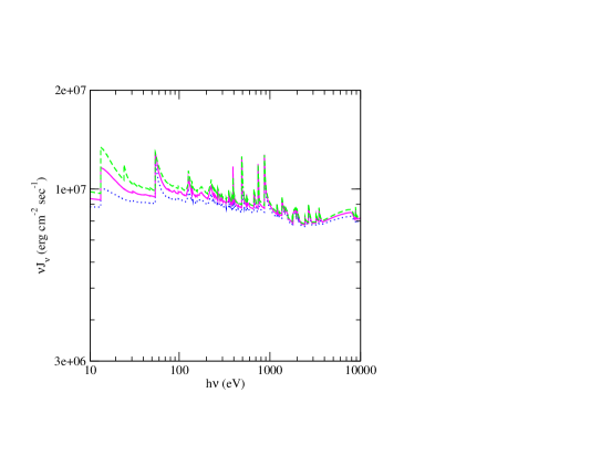
Figure 1: This figure displays the spectral distribution of the mean continuum intensity, computed at the illuminated surface of the slab, for three “intermediate” models: MI 1_I (dotted line), MI 2_I (solid line), and MI 3_I (dashed line). For the sake of clarity, the spectral lines have been supressed from this figure, where only the continuum is shown; this displays important discontinuities, which increase with the slab thickness.

2.2 Different computational methods used

We recall that the set of equations describing the physical state of the gas (i.e. the local balance between the ionization and recombination processes, excitations and de-excitations, as well as the local energy balance) is computed at each depth in the gas slab. In TITAN‘s previous computational scheme, the thermal energy balance equation was solved for a given density at a given depth (that of the previous iteration); this method provides a unique solution for the temperature. The model corresponding to this scheme will be called “intermediate” model hereafter.

In the new version of TITAN, the energy balance equation is solved for a given total pressure, assumed to be constant along the slab. In some regions of the cloud, this computational scheme leads to two stable solutions, described by two separate models. In one of the models, the “hot” solution is systematically chosen for all layers, while in the other model the “cold” solution is systematically preferred. These models will be called hereafter “hot” model and “cold” model, respectively. They actually represent two extreme results corresponding to a given gas composition and photoionizing flux, being compatible with the two stable solutions. It is important to stress that these models differ not only in the layers where multiple solutions are possible, but all along the gas slab, this because the entire radiation field will be modified in a thick medium.

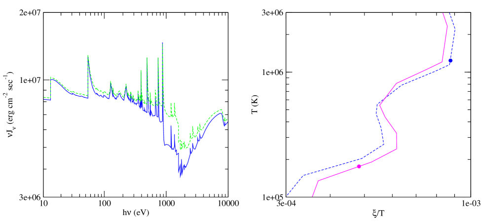
Figure 2: This figure displays some results obtained for an “intermediate” model with $\xi=1000$ and $N_{\rm H}=2\,10^{23}$ cm^-2 (MI 1_I). On the left-hand panel we give the spectral distribution of the mean continuum for two layers located at different depths in the gas slab; these layers correspond to a column density value of 1.66 10²³ (dashed line) and 1.90 10²³ (solid line). On the right-hand panel, we display the S-curves giving $T$ versus  $\xi/T$ for the same two layers (the same line-codes apply); the dots represent the equilibrium temperature found for each layer.

This, and other behaviours of a slab of optically thick gas in constant pressure equilibrium, will be discussed in the following sections. We have chosen to work with a few models encompassing the range of conditions valid for the Warm Absorber in AGN; they are given in Table 1. The same study could, of course, be performed for a different set of values; this would not change our main results and conclusions.

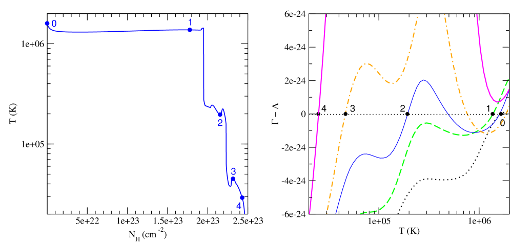
Figure 3: On the left-hand panel we give the temperature profile along the slab (i.e., versus the column density), for the model MI 2 ($\xi=1000$, $N_{\rm H}=2.5\,10^{23}$) computed with the “cold” solution. The dots represent gas at different depths in the slab, for which we have plotted the corresponding cooling curves on the right-hand panel. We observe that the net cooling function $\cal{L}$ has one single solution for the layers labelled 0, 1 and 4 in the slab, while there are three possible solutions for the layers labelled 2 and 3; from these, only the “cold” solution was selected to compute the gas structure and spectra.

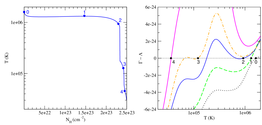
Figure 4: Same as in Fig. 3, except the model has been computed with the “hot” solution. In the right-hand panel, layers labelled 2 and 3 display three possible solutions, from which the “hot” one has been systematically choosen; the layers labelled 0, 1, and 4 display a single solution.

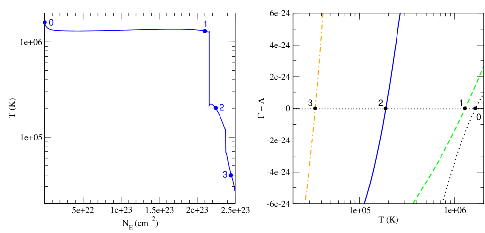
Figure 5: Same as in Figs. 3 and 4, except the model has been computed with the “intermediate” solution. In this case, the cooling curves in the right-hand panel always provide a unique solution, independently of the depth of the layer considered (dots on the left-hand panel).

3 The models

All the models presented here were treated in a 1-D plane-parallel geometry, as slabs of gas illuminated from one side by a radiation field concentrated in a very small, pencil-like, shape centered on the normal direction. The resultant spectrum, reprocessed by the gas, is a combination of “reflection” from the illuminated side of the medium (not a real reflection, as it includes atomic and Compton reprocessing), “outward emission” (coming from the non-illuminated side of the medium), and a “transmitted” fraction of the incident ionizing continuum. The absorption spectrum (which corresponds to the outward emission in the normal direction) depends strongly on the column density, since the cool absorbing layers are located at the back side of the gas slab. The relative contribution of each component to the observed spectrum depends on parameters such as the size, the density, and the geometry of the ionized medium.

Our models are globally parameterized by the column density $N_{\rm H}$ (in units of cm^-2), the hydrogen number density at the illuminated side of the slab $n_{\rm H}$ (in units of cm^-3), the incident flux and SED, and the ionization parameter; this parameter is defined differently among authors. In this article, we use the $\xi$ form of the ionization parameter, where

$$\xi=\frac{L}{n_{\rm H}R^{2}}\ \ \leavevmode\nobreak\ \leavevmode\nobreak\ \leavevmode\nobreak\ \leavevmode\nobreak\ \leavevmode\nobreak\ \leavevmode\nobreak\ {\rm(in\ units\ of\ erg\leavevmode\nobreak\ cm\leavevmode\nobreak\ s^{-1})}$$ (3)

in which $R$ is the distance between the radiating source and the photoionized medium, and $L$ is the source’s bolometric luminosity (in erg s^-1); in the following, we integrate $L$ over the range 10$-$10⁵ eV, but some authors prefer to give $\xi$ with $L$ integrated over the 1$-$1000 Ryd region, as used by XSTAR. Appropriate conversions should thus be applied if using different forms of the ionization parameter, and before any numerical comparison. Note that $\xi$, as well as $n_{\rm H}$, are quantities defined at the illuminated surface of the slab. We recall that in constant pressure models the hydrogen number density varies along the slab, displaying a profile varying inversely with the temperature; also the spectral distribution of the ionizing radiation changes across the slab for media in pressure equilibrium, as those discussed in this paper.

All our models were computed under total (i.e., gas plus radiation) pressure equilibrium; we have neglected all other forms of pressure (e.g., turbulent, magnetic, …) contributing to the total pressure. The gas slabs were assumed to have cosmic abundances (Allen 1973); the hydrogen numerical density at the illuminated surface was set to $10^{7}$ cm^-3. Note that $n_{H}$ is a minor parameter in this study, the overall spectrum being only proportional for values varying from 10⁷ to 10¹² cm^-3 (this is usually the case, provided the ionizing spectrum is relativelly flat); only the relative intensities of the forbidden and permitted emission lines (e.g., from He-like ions like O vii) are sensitive to changes in the density.

We have simplified our models by assuming a null turbulent velocity component; micro-turbulence has a small influence on the thermal and ionization structure for large column densities, where the cooling is dominated by bound-free transitions. The thermal and ionization structures are mainly determined by the ionization parameter and the shape of the ionizing continuum. All the models in this paper assume an incident continuum described by a power-law of photon index $\Gamma=2$, covering the 10$-$10⁵ eV energy range.

4 “Hot”, “cold”, and “intermediate” solutions

In this section, we illustrate the differences between the previously discussed computational methods by comparing the results obtained with the “hot”, “cold”, and “intermediate” models.

4.1 Behaviour at the surface of the gas slab

It is often assumed that the thermal instability problem in thick media is exactly the same as in thin media. This is not true, for mainly two reasons. First, the spectral distribution of the mean intensity $J_{\nu}$ at the illuminated surface of the slab is different from the incident spectrum, as it equally contains a “returning” radiation component emitted by the slab itself. As an illustration, Fig. 1 shows the spectral distribution of the mean continuum intensity at the slab surface for three “intermediate” models with $\xi=1000$ and 3 different values of the column density. For the sake of clarity, the spectral lines were suppressed from the figure, and only the continuum is shown. We observe that the spectrum at the surface contains strong discontinuities, whose amplitude increases with the slab thickness. More generally, the intensity of the whole spectrum increases with the slab thickness (an expected behaviour since the radiation emitted by a thicker slab should be larger). Second, the spectral distribution changes as the radiation progresses inside the medium. As a consequence, the shape of the S-curve also changes, and instead of traveling along a given S-curve as $P_{\rm rad}/P_{\rm gas}$ decreases, the temperature follows successively different curves. This behaviour is illustrated by the MI 1_I model in Fig. 2, which shows the spectral distribution of the mean continuum for two layers located at different depths in the gas slab (left-hand panel) and the corresponding curves giving $T$ versus $\xi/T$ (right-hand panel), which is the same as representing the usual S-shape curve. We can see that the S-curves are different for the two represented layers and, in particular, that the curve corresponding to the deeper layer (solid line) displays a larger multi-branch region; this is due to its larger absorption trough. The dots represent the equilibrium temperature found for each layer.

4.2 Comparison between cooling curves

Figures 3, 4, and 5 concern a slab of gas with total column density equal to $2.5\ 10^{23}$ cm^-2, ionized by an incident continuum with $\xi=1000$ (MI 2 model). These figures display, for respectively the “cold”, “hot”, and “intermediate” solution models, the temperature profile versus the column density (left-hand panel) and the net cooling function (${\cal{L}}=\Lambda-\Gamma$) versus the temperature, at different depths in the gas slab (right-hand panel); the various layers represented here have been marked and labelled in the left-hand panel. By comparing both plots we can verify that $\cal{L}$ cancels for the equilibrium temperatures observed in the gas structure.

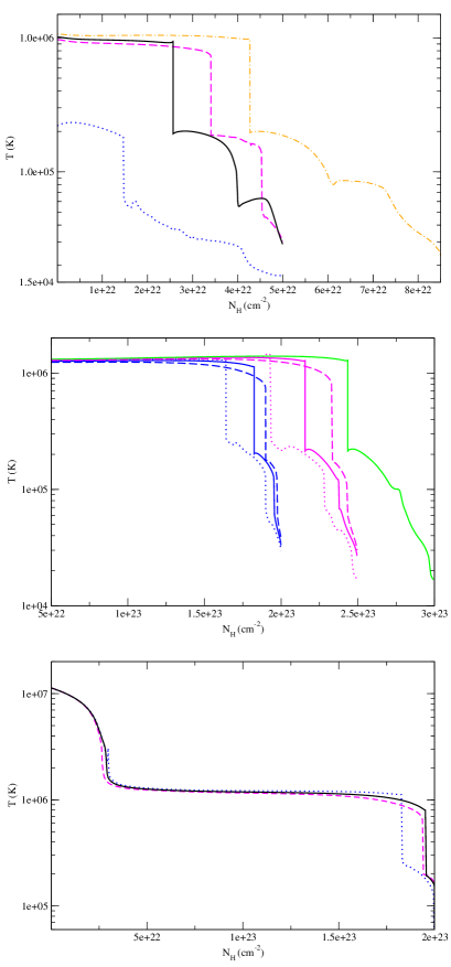
Figure 6: Temperature profiles versus the column density for a set of models with different $\xi$ and $N_{\rm H}$. On the top panel, the LI 1 models (dashed line: “hot” solution; dotted line: “cold” solution; solid line: “intermediate” solution); for comparison, we also plotted the LI 2_I model (dashed-dotted line). On the middle panel, several MI models for different values of the column density (dashed lines: “hot” solution models; dotted lines: “cold” solution models; solid lines: “intermediate” solution models). Finally, on the bottom panel, the HI 1 models (the same line-codes apply).

We recall that the cooling curves of the “hot” and “cold” models are determined for a given total pressure, while those of the “intermediate” models are computed for a given density. We can check that the isobaric cooling curves of the “cold” and “hot” models (Figs. 3 and 4, respectively) display three solutions for ${\cal{L}}=0$, while the isodensity cooling curves of the “intermediate” model (Fig. 5) always show a unique solution. We stress that it is impossible to compare the cooling curves in exactly the same conditions, as the models computed with these three solutions differ considerably. Indeed, the radiation field is completely different in the three models, even at the illuminated surface layer; therefore, the isobaric cooling curves differ strongly, even for a layer located at a similar depth in the gas slab.

Let us examine first the cooling curves corresponding to the “cold” model (Fig. 3). We can see that, at the illuminated surface and at position 1, there is a unique solution, while at positions 2 and 3 there are three possible solutions, from which the coldest one is chosen; near the back surface of the slab, at position 4, the solution is again unique. Similarly, for the “hot” model (Fig. 4), the solution is unique at the surface and at position 1, but at positions 2 and 3 the curve has three solutions, from which the hotter one is chosen; then, at position 4, again the solution is unique. However, the multi-branch region is different in the case of the “hot” or the “cold” model; this shows how much these two models differ. Finally, in the case of the “intermediate” model (Fig. 5), all solutions are unique. Given these differences, we would expect that the previous computational scheme used by TITAN, with its isodensity cooling curves, would be completely wrong; this is not the case, as we will see later on. Indeed, such a method provides temperature structures and spectra which are intermediate between those of the “cold” and the “hot” models.

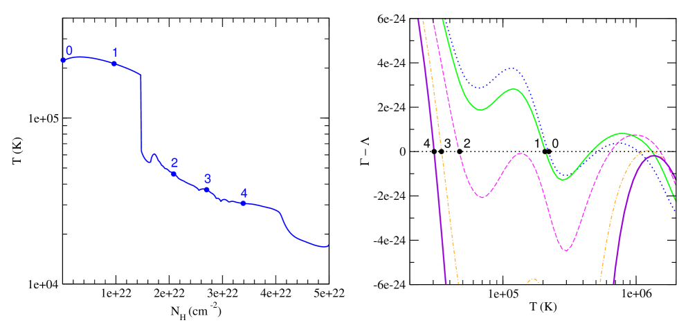
Figure 7: Temperature profile versus the column density for a model with $\xi=300$ and $N_{\rm H}=5\,10^{22}$ (left-hand panel). We have marked several layers, corresponding to different positions in the gas slab, labelled from 0 (at the illuminated surface) to 4 (deeper in the slab). On the right-hand panel, we give the corresponding cooling curves, which display one (position 4) or more solutions. It is interesting to note that, at such low ionizations, the surface layer is already in the multi-solutions regime, displaying 3 possible solutions from which the coldest one has been chosen.

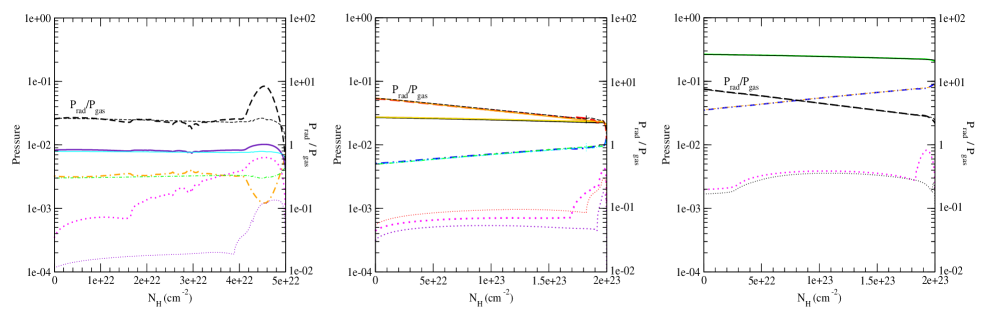
Figure 8: This figure shows various pressure quantities computed with the “cold” (thick lines), “hot” (thin lines), and “intermediate” (thinner lines) solutions for the models LI 1 (left-hand panel), MI 1 (middle panel), and HI 1 (right-hand panel). For the sake of clarity, the “intermediate” solution values are only shown for one of the models (MI 1, middle panel). In all the panels, $P_{\rm rad}$ is given in solid lines, $P_{\rm gas}$ in dashed-dotted lines, $P_{\rm rad}({\rm lines})$ in dotted lines, and the $P_{\rm rad}/P_{\rm gas}$ ratio in dashed lines; also, the left-hand y-axis (10^-4 $-$ 1) corresponds to the $P_{\rm rad}$, $P_{\rm gas}$, and $P_{\rm rad}({\rm lines})$ values, while the right-hand y-axis (10^-2 $-$ 10²) corresponds to the $P_{\rm rad}/P_{\rm gas}$ ratio.

4.3 Temperature profiles

Figure 6 displays the temperature profiles for the “cold”, “hot”, and “intermediate” solutions, for a set of LI ($\xi=300$), MI ($\xi=1000$), and HI ($\xi=10000$) models. The “intermediate” solutions are represented by solid lines (on the top panel, the LI 2_I model was represented by a dashed-dotted line for the sake of clarity), the “cold” solutions by dotted lines, and the “hot” solutions by dashed lines. By analysing this figure, two results appear clearly:

• First, the differences between the “hot”, “cold”, and “intermediate” models increase as $\xi$ decreases;

• Second, the temperature always decreases strongly near the non-illuminated surface of the slab, whatever the column density.

In the following, we will present some clues allowing to understand these behaviors.

4.3.1 Influence of the ionization parameter

For the higher ionization models ($\xi=10000$), the “hot”, “cold”, and “intermediate” solutions provide very similar results (cf. Fig. 6, bottom panel). On the contrary, for the lower ionization models ($\xi=300$) the results are quite different, the first layer at the illuminated side of the slab being already in the multi-solutions regime (cf. Figure 6, top panel). In this case, since the “hot” and “cold” solutions correspond to very different equilibrium temperatures, there is also a large difference on the whole medium structure. This is illustrated by Fig. 7, which is similar to figures 3, 4 and 5, except we now address the case of the LI 1 “cold” solution model. The figure shows that, already at the illuminated surface of the slab (labelled 0 on the left-hand panel), the net cooling curve cancels for three values of the temperature; this multi-solutions regime lasts until the deeper position labelled 4 on the left-hand panel.

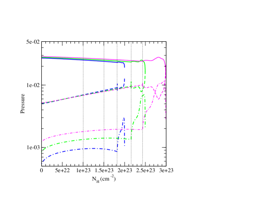
Figure 9: Figure showing the variation of $P_{\rm rad}$, $P_{\rm rad}({\rm lines})$, and $P_{\rm gas}$ versus the column density, for 3 “intermediate” models of different thickness (MI 1, MI 2, and MI 3). $P_{\rm rad}$ is represented by solid lines, $P_{\rm gas}$ by dashed lines, and $P_{\rm rad}({\rm lines})$ by dashed-dotted lines. The variation of $P_{\rm rad}$ along the gas slab is very similar for the three different thicknesses, until the first temperature jump occurs. We also observe that near the back side of the gas slab, $P_{\rm rad}$ can become very important, owing to the contribution from the lines. The thin dotted vertical lines represent layers at different depths in the slab, corresponding namely to $1\,10^{23}$ cm^-2, 1.5 $10^{23}$ cm^-2, and to the first temperature jump in each model (1.82 $10^{23}$, 2.16 $10^{23}$, and 2.43 $10^{23}$ cm^-2 for the MI 1, MI 2, and MI 3 model, respectively).

It is possible to address this situation and try to find an adequate explanation for the behaviour of the LI 1 model by looking into what’s happening with the $\Xi$ ionization parameter (or, which is similar, studying the $P_{\rm rad}/P_{\rm gas}$ ratio). Since the multi-solutions regime occurs for a given range in $\Xi$, one expects that the associated region in the slab would correspond to layers where $P_{\rm rad}/P_{\rm gas}$ is of the order of a few units. This is indeed the case, as shown in Fig. 8. This figure displays the variation of $P_{\rm rad}$, $P_{\rm gas}$, and $P_{\rm rad}/P_{\rm gas}$ along the slab, for the “hot” and “cold” solutions of a set of LI, MI, and HI models. The radiation pressure due to the lines, $P_{\rm rad}({\rm lines})$, is also shown, as this component can be quite important near the back side of the slab; note that $P_{\rm rad}$, also represented in the figure, already includes the contribution from $P_{\rm rad}({\rm lines})$. In this figure, the “cold”, “hot”, and “intermediate” models are represented by thick (green, black, violet), thin (blue, orange, magenta), and very thin lines (cyan, yellow, red), respectively. $P_{\rm rad}$ is given in solid lines, $P_{\rm gas}$ in dashed-dotted lines, $P_{\rm rad}({\rm lines})$ in dotted lines, and the $P_{\rm rad}/P_{\rm gas}$ ratio in dashed lines. The left-hand y-axis (10^-4 $-$ 1) corresponds to the $P_{\rm rad}$, $P_{\rm gas}$, and $P_{\rm rad}({\rm lines})$ values, while the right-hand y-axis (10^-2 $-$ 10²) corresponds to the $P_{\rm rad}/P_{\rm gas}$ ratio. For the sake of clarity, the “intermediate” solution values (thinner lines: cyan, yellow, red) are only shown for one of the models (MI 1, in the middle panel).

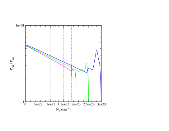
Figure 10: Figure showing the $P_{\rm rad}/P_{\rm gas}$ ratio versus the column density, for the 3 “intermediate” models discussed in the previous figure. This ratio decreases as we penetrate in the gas slab until it reaches a value $\sim$2.5, coinciding with a temperature jump. The figure shows that this ratio decreases more rapidly for the thinner, than for the thicker gas slab. The thin dotted vertical lines represent layers at different depths in the slab (same as in Fig. 9).

Observing Fig. 8, we first notice that, in all cases, the pressure is entirely dominated by $P_{\rm rad}$, and that $P_{\rm rad}/P_{\rm gas}$ at the illuminated surface increases with $\xi$, as expected. The $P_{\rm rad}/P_{\rm gas}$ ratio decreases accross the slab from the illuminated surface to the back side as the radiation is absorbed, the slab entering the multi-solutions regime when $P_{\rm rad}/P_{\rm gas}$ is of the order of 2.5; this is true whatever the pressure ratio at the illuminated side. It is easy to see that such a value was promply attained in the case of the LI 1 model discussed before; as a consequence, we were able to observe a “cold” and a “hot” solution already at the surface of the slab.

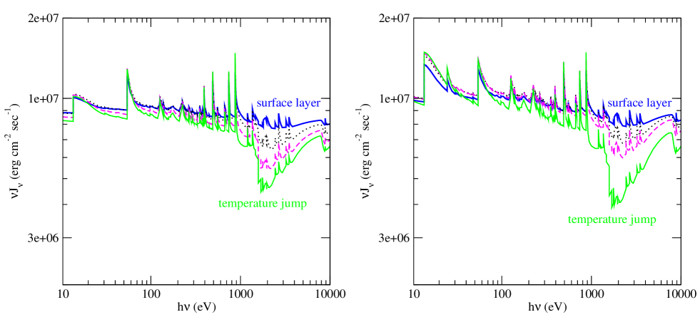
Figure 11: Figure showing the medium intensity spectral distribution for two MI “intermediate” models with different column densities: on the left-hand panel, the thiner (shorter) model with $N_{\rm H}=2\,10^{23}$; on the right-hand panel, the thicker (longer) model with $N_{\rm H}=3\,10^{23}$. Both panels display the spectral distribution corresponding to 4 layers, from the illuminated surface of the slab (top curves) to the layer closer to the temperature jump (bottom curves).

It is also interesting to note that, in spite of a big difference in temperature, the gas pressure at the surface is almost the same for the “cold” and “hot” models. This behaviour is actually due to an automatic adjustment of the density, which is equal to $5\,10^{7}$ cm^-3 in the first layer of the “cold” model, instead of the smaller, initial value of $10^{7}$ cm^-3. The figure also shows that, for all values of the ionization parameter, the pressures in the three models (“cold”, “hot”, and “intermediate”) are quite similar, except for $P_{\rm rad}({\rm lines})$ near the back side of the slab. Indeed, the contribution from the lines is always less important in a hot medium than in a cold medium, which can emit intense ultraviolet lines. Therefore, the smaller the ionization parameter, the more important are the lines. It is thus easy to understand how $P_{\rm rad}({\rm lines})$ can even dominate the radiation pressure near the back side of the the LI 1_C model (cf. Fig. 8, left-hand panel).

Note finally that the sharp temperature drops, observed in the left-hand panel of figures 3, 4, 5 and 7, do not occur exactly at the same value of $P_{\rm rad}/P_{\rm gas}$ for all the models; this is due to the shape of the S-curve, and to the different spectral distributions inside the slab, which depend not only on the type of model (“cold” or “hot”), but also on the ionization parameter and on the total tickness of the medium.

4.3.2 Influence of the medium thickness

As already noted by Różańska et al. (2006) and Chevallier et al. (2006a), the thickness of a pressure equilibrium medium cannot exceed a maximum value for a given ionization parameter. This is explained by the fact that, when the temperature reaches low values (of the order of 10⁴ K), the radiation pressure becomes dominated by the spectral lines, and therefore the gas enters in a new multi-solutions regime. When the temperature drops to the cold values corresponding to a molecular gas, we reach a limit and are unable to provide a solution, as our code cannot handle molecular gas.

If the maximum thickness of a medium in pressure equilibrium is a known issue, there are two other puzzling problems related to the thickness of the slab. The first is related to the fact that the temperature always decreases rapidly near the non-illuminated side of the gas slab. The second concerns the reason why the slab always enters a multi-solutions regime just before the slab ends, even when the imposed column density is much smaller than the possible maximum value.

We are going to address these issues using the “intermediate” solution models as an illustration. Let us consider a set of models with $\xi=1000$. Figure 9 displays the variation of $P_{\rm rad}$, $P_{\rm rad}({\rm lines})$, and $P_{\rm gas}$ along the slab for three values of the column density. $P_{\rm rad}$ is represented by solid lines, $P_{\rm gas}$ by dashed lines, and $P_{\rm rad}({\rm lines})$ by dashed-dotted lines. We can see that the dependence of $P_{\rm rad}$ — and therefore also of $P_{\rm gas}$, since the sum of $P_{\rm rad}$ and $P_{\rm gas}$ is constant — on the gas position inside the slab is almost the same for the three different thicknesses until the first temperature jump occurs. For the sake of simplicity, we do not show here $P_{\rm rad}/P_{\rm gas}$, but it is clear that this ratio displays always approximately the same value ($\sim$ 2.5) at the temperature jump (the position of the temperature jump can be seen in Fig. 6, middle panel). Such temperature changes are accompanied by a strong increase in $P_{\rm rad}({\rm lines})$. The thicker the slab, the larger is the cold zone, and the stronger the increase in $P_{\rm rad}({\rm lines})$. One can even observe an inversion of the gas pressure variation near the back surface of the slab, for the thickest case (MI 3 model). Very close to the back surface, the layers are optically thin for the continuum and the lines, which can thus escape from the medium; this induces a rapid decrease in the radiation pressure, as observed in the figure; it also leads to a strong cooling, causing a rapid decrease of the temperature near the back surface of the slab. These coupled phenomena give an answer to the first problem.

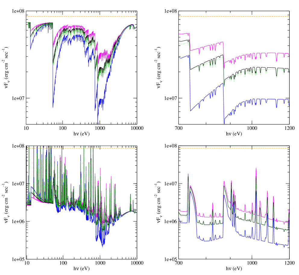
Figure 12: This figure gives the pure absorption (top panels) and outward emission spectra (bottom panels) for the MI 1 model. The “cold” solution model is represented by the lower blue lines, the “hot” model by upper magenta lines and the “intermediate” model by the middle black lines; the spectra corresponding to the half-sum of the “hot” and “cold” models are also plotted for comparison (green dotted lines). The orange dashed line corresponds to the incident ionizing continuum. The spectra are represented with a resolution of 300; the right-hand panel foccuses on the 700$-$1200 eV energy range for details, while the left-hand panel shows a larger band covering the 10 $-$ 10⁴ eV range. Notice the excellent agreement between the “intermediate” and half-sum spectra over the entire energy range.

The second issue is more subtile. From Fig. 9 we know that $P_{\rm rad}$ decreases inside the slab (except near the back side, owing to the lines, as explained). Since $P_{\rm rad}$ is slightly larger in thicker slabs, the traversed length before reaching the ratio $P_{\rm rad}/P_{\rm gas}$ required for the temperature jump, is larger for thicker slabs. However, this is not sufficient to explain why the temperature transition is located closer to the illuminated surface in thiner slabs, or the difference between the transition positions would not be so large in media with different thicknesses. Additional explanation can be found in Fig. 10, which compares the $P_{\rm rad}/P_{\rm gas}$ ratio versus the position in the slab (given in terms of column density) for the same three slab thicknesses discussed in the previous figure; we can see that this ratio decreases more rapidly for the thinner (i.e. shorter), than for the thicker (longer) gas slab.

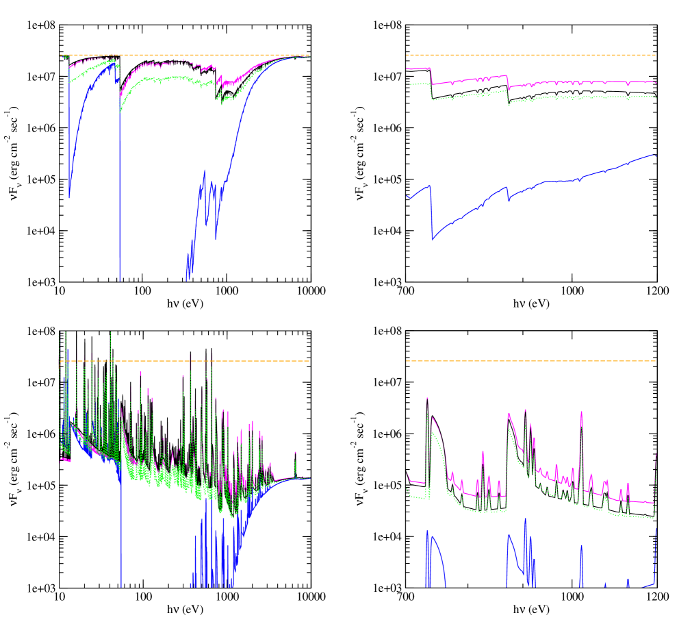
Figure 13: Same as in the previous figure, only for the lower ionization model LI 1. In this case, the agreement between the “intermediate” and half-sum spectra is not as good as for the MI 1 model. The differences are less important for the outward emission in the X-ray range.

The explanation for this behaviour can be found in the comparison between the spectral distribution of the first layer, and of a layer located close to the place where the jump in temperature occurs. Figure 11 displays the spectral distribution of the mean intensity (again, the lines were suppessed for clarity), for two MI, “intermediate” models with total column densities 2 10²³ cm^-2 (left-hand panel) and 3 10²³ cm^-2 (righ-hand panel), at different positions in the slab (from top to bottom: at the illuminated surface, at $1\,10^{23}$ cm^-2, $1.5\,10^{23}$ cm^-2, and at the first temperature jump — $1.82\,10^{23}$ for MI 1 and $2.43\,10^{23}$ for MI 3); these layers are identified in Fig. 10 by thin vertical dotted lines. We can observe that the spectral distribution of the continuum varies differently in the two media: at the same location in the slab, the spectrum is less absorbed in the thicker slab (righ-hand panel), owing to the more important re-emission component. In other words, the spectral distribution of the thiner, shorter slab (left-hand panel) has a stronger trough, and reaches more rapidly the multi-solutions regime, as explained above (cf. Fig. 2).

5 Observational implications

5.1 Outward emitted and absorbed spectra

Unfortunately, it is impossible to know what solution the plasma will adopt when attaining the multi-solutions regime. For instance, it can oscillate between the hot and cold solutions, it can fragment into hot and cold clumps which will coexist together, or it can take the form of a hot, dilute medium confining cold, denser clumps (the hot and cold media sharing the same pressure). We recall that the “cold” and “hot” models computed by TITAN can be interpreted as “extreme” models, as they adopt respectively the “cold” or the “hot” solutions all along the slab. The spectra emitted or absorbed by a given ionized medium, consisting of a mixture of gas in the hot and cold phases, should thus be intermediate between those resulting from the pure “cold” and “hot” models. The differences between the emitted and absorbed spectra obtained with the stable solutions can thus provide an indication for the maximum “error bars” associated to the spectra computed with the “intermediate” solution.

As an example, Figs. 12 and 13 give the pure absorption (top panels) and outward emission (bottom panels) spectra resulting from the “cold”, “hot”, and “intermediate” (black, middle curves) solutions for the MI 2 and LI 1 models, respectively (see Fig. 6 for the corresponding temperature profiles). The spectra are represented with a resolution of 300 and have been displayed in two energy ranges: 10$-$10⁴ eV (left-hand panels), with a zoom in the 700$-$1200 eV region (right-hand panel) to more clearly observe the differences. The lower solid lines (blue) correspond to the “cold” models, the middle lines (black) to the “intermediate” models, and the upper lines (magenta) to the “hot” models. The incident ionizing continuum (orange dashed lines) and the spectrum corresponding to the half-sum of the “cold” and “hot” models (green dotted lines) are also plotted, for comparison. The outward emission spectrum has been computed for an opening angle of 45 degrees which, according to the unified Scheme of AGN (Antonucci & Miller 1985), is in agreement with the expected geometry for the Warm Absorber in Seyfert 1 nuclei, or the emissive region in Seyfert 2s.

Investigating the MI 2 spectra in Fig. 12, we can see that the “intermediate” model spectra (black solid lines, middle) is extraordinary close to the half-sum (green dotted lines) of the “cold” and “hot” spectra, though these ones are quite different. The differences amount at most to 1 or 2% for the outward emitted spectrum, and to 20% for the absorption spectrum. The agreement is not as good for the second case (LI 1 model, Fig. 13), where the differences between the “intermediate” model and the half-sum of the “cold” and “hot” models amount typically to a factor 2 for the absorption spectrum. The agreement is much better for the outward emission in the X-ray range. This is due to the strong imprint of the cold layers near the back surface of the “cold” model, which absorb almost completely the UV-X spectrum. On the contrary, the X-ray outward emission, being due mainly to the deep layers, is not very different for the “hot” and the “cold” models.

We observe that the lines have similar intensities in the “cold” and “hot” spectra, and also in the “intermediate” and half-sum spectra; this happens in spite of important differences in the continuum intensity, in particular for the ionization edges. Such a behaviour is due to the fact that the main lines are saturated resonance transitions, while the ionization edges are optically thiner, and therefore almost proportional to the thickness of the region containing the emitting ion (apart from the diffuse emission contribution).

5.2 Ionization states

Differences in the ionization state for “hot” and “cold” models are illustrated by Fig. 14, which displays the fractional ionization of two important elements — Si (top panels) and O (bottom panels) — for the “cold” (left-hand panels) and “hot” (right-hand panels) models already depicted in Fig. 12. This figure clearly shows why the intensities of the ionization edges are different in the “cold” and “hot” models. We can see that the length of the O vii and O viii regions is about three times larger in the “cold” model than it is in the “hot” model, these differences being somewhat larger than the discrepancy in the corresponding spectra.

5.3 Variability

In the multi-solutions regime, the medium should be made of a mixture of gas in the hot and cold phases, and the relative proportion of those phases could be varying with time. The whole medium should thus oscillate between physical states located somewhere in the parameters’ region covered by the “hot” and “cold” models. The variation timescale in such a medium is basically the thermal time in the multi-branch region. However, if the medium is subject to a change in temperature, this will not necessarily be immediately followed by a change in ionization inducing modifications in the main absorbing or emitting ions. It all depends on the relative values of the thermal time $t_{\rm th}$, the ionization time $t_{\rm ion}$ and the recombination time $t_{\rm rec}$. One thus expects two types of variability: a relativelly weak variability related only to a temperature variation, and a stronger variability related to a change of ionization state. If $t_{\rm ion}$ or $t_{\rm rec}$ are smaller than $t_{\rm th}$, strong variations in the emitted/absorbed spectrum should be observed during the thermal time-scale, with the main emission/absorption lines and ionization edges being replaced by lines and edges of other ions. If $t_{\rm ion}$ and $t_{\rm rec}$ are larger than $t_{\rm th}$, the spectrum should display smaller changes, like a simple variation in the relative intensity of the spectral features.

Let us compare these three timescales. The thermal time $t_{\rm th}$ is of the order of $kT/n{\Lambda}$. In the multi-solutions regime, the cooling and the heating are dominated by atomic processes, and $\Lambda$ is of the order of 10^-23 erg cm³ s^-1, so $t_{\rm th}$ writes:

$$t_{\rm th}\sim{T_{5}\over n_{12}\,{\Lambda_{23}}}\ \ \ \ {\rm(in\leavevmode\nobreak\ units\leavevmode\nobreak\ of\leavevmode\nobreak\ s)},$$ (4)

where $n_{12}$ is the density expressed in 10¹² cm^-3, ${\Lambda}_{23}$ is the cooling function in 10^-23 erg cm³ s^-1, and $T_{5}$ is the temperature in 10⁵ K.

For a given ion, $t_{\rm rec}$ is equal to $t_{\rm rec}=1/(n_{\rm e}\,\alpha_{\rm ion})$ where $n_{\rm e}$ is the electron numerical density (roughly equal to the total density $n$), and $\alpha_{\rm ion}$ is the recombination coefficient of the given ion, including dielectronic recombinations. This coefficient is almost independent from the radiation flux, with a typical value of 10^-11 cm³ s^-1 at the temperature of the multi-branch region for a heavy, highly ionized element, so $t_{\rm rec}$ writes:

$$t_{\rm rec}\sim{0.1\over n_{12}\,\alpha_{11}}\ \ \ \ {\rm(in\leavevmode\nobreak\ units\leavevmode\nobreak\ of\leavevmode\nobreak\ s)},$$ (5)

where the recombination coefficient $\alpha_{11}$ is expressed in 10^-11 cm³ s^-1. Thus, the recombination time $t_{\rm rec}$ of a heavy element in a highly ionized state is smaller than, or of the order of, the thermal time $t_{\rm th}$. One deduces that a thermal variation induces almost immediately a change in the ionization state.

Ionization equilibrium is reached after a time equal to the maximum time-scales given by $t_{\rm ion}$ and $t_{\rm rec}$. The ionization time $t_{\rm ion}$ is defined as:

$$t_{\rm ion}=\left(\int_{\nu({\rm ion})}^{\nu({\rm max})}{4\pi\,{J_{\nu}\over h\nu}\,\sigma_{\nu}\,d\nu}\right)^{-1},$$ (6)

where $\sigma_{\nu}$ is the frequency-dependent photoionization cross-section of the given ion. As we have seen, $J_{\nu}$ varies across the slab, but we can make a very rough estimation of $t_{\rm ion}$ by assuming that $J_{\nu}$ is of the order of the incident flux, $F_{\nu}/2\pi$. This could lead to a large overestimation of the ionization rate, and therefore to an underestimation of the ionization time, as $J_{\nu}$ is actually smaller than $F_{\nu}/2\pi$ in the deep layers, at the back of the slab (cf. the outward emitted spectrum in Figs. 12 and 13). With our power law incident spectrum described by $F_{\nu}\propto\nu^{-1}$ in the 10$-$10^-5 eV range, and assuming that the cross-section is proportional to $\nu^{-3}$, one finds:

$$t_{\rm ion}\sim{3\ 10^{-5}\over\xi_{3}\,n_{12}\,\sigma_{19}}\ \ \ \ {\rm(in\leavevmode\nobreak\ units\leavevmode\nobreak\ of\leavevmode\nobreak\ s)},$$ (7)

where $\xi_{3}$ is the ionization parameter $\xi$ expressed in 10³ erg cm s^-1 and $\sigma_{19}$ is the cross-section at the ionization edge of the given ion expressed in 10^-19 cm^-2.

In conclusion, even if it may be underestimated by two orders of magnitude, $t_{\rm ion}$ is smaller than $t_{\rm rec}$, and both time-scales are smaller than $t_{\rm th}$; therefore, if the temperature changes locally in the multi-branch region, a new ionization equilibrium settles in immediately.

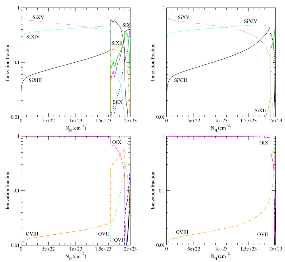
Figure 14: Figure showing the fractional ionization of the Si ions (top panels) and O ions (bottom panels) for the same models as in Fig. 12. The “cold” and “hot” models are displayed in the left-hand panels and right-hand panels, respectively. We observe that the regions producing the various ions have important size differences in the case of a “cold”, or of a “hot” model.

The problem is more complex in practice. Indeed, in order to observe variations in the spectrum, the change of temperature should affect a large proportion of the multi-branch region. The mass fractions of the hot and cold phases are most probably of the same order, so this zone should be made of cold, dense clumps embedded in a hotter and more dilute medium. In this case, the evaporation time of the clumps should govern the structural changes. This time-scale is of the order of the cold phase dynamical time, if evaporation is not saturated.

The dynamical time is roughly equal to $\Delta H/c_{\rm s}$, where $\Delta H$ is the thickness of the multi-branch region, and $c_{\rm s}$ is the sound velocity in the cold phase. The sound velocity includes the radiation pressure, but in a proportion which depends on the relation between the radiation field and the gas. Since the multi-branch region is not very optically thick, one can neglect the radiation pressure, and simply assume $c_{\rm s}=\sqrt{2kT/m_{\rm H}}$, where $m_{\rm H}$ is the proton mass. The thickness of the multi-branch region is a fraction $f_{\rm multi}$ of the total thickness of the slab, which itself depends on the density (since the column density is a given parameter). Expressing the total column density in 10²³ cm^-2, one finds:

$$t_{\rm dyn}\sim 2\ 10^{4}\,{f_{\rm multi}\,N_{23}\over\sqrt{T_{5}}\,n_{12}}\ \ \ \ {\rm(in\leavevmode\nobreak\ units\leavevmode\nobreak\ of\leavevmode\nobreak\ s)}.$$ (8)

It is interesting to note that all timescales depend on the same way on the density, which is often an unknown parameter when dealing with observational data (e.g., Warm Absorber gas). If the timescales vary for different locations in the slab (because the density value is not the same at different depths), their ratio does not change much. In particular, the ratio $t_{\rm dyn}/t_{\rm th}$ is very large (of the order of 10³ if the thermal instability affects 10% of the slab), therefore the multi-branch region should contain local thermal perturbations out of pressure equilibrium.

Chevallier et al. (2006b) made a detailed study on the viability of pressure equilibrium media in the presence of variations of the incident radiation flux. The authors have shown that, though the global pressure equilibrium is generally preserved (with the medium responding to the variations by rapidly adjusting its ionization and thermal equilibrium), supersonic velocities develop in the gas, owing to local over- or under-pressure states. The same phenomenon should occur in the multi-branch region of our media, even in the absence of incident flux variations. To study this problem, a complete perturbational study should be performed around the equilibrium state of the gas slab; such a study is out of the scope of the present paper. For the time being, we can just conclude that large spectral fluctuations corresponding to the onset of a “cold” or a “hot” solution could be observed in timescales of the order of the dynamical time, independently of any variation of the radiation field external to the medium. Moreover, a strong turbulence implying supersonic velocities leading to line broadening should permanently exist in the multi-branch region of thick, stratified, pressure equilibrium media.

5.4 Practical considerations

An important point to take into account when choosing which computational method to apply, is that the full computation of the “hot” and “cold” models described here is extremely time-consuming; this is because the process is strongly unstable and requires thus more iterations than the isodensity scheme models. Given the results presented in this paper, it seems thus reasonable to use the simpler, isodensity scheme to compute constant pressure models or hydrostatic equilibrium models. This procedure is less ad-hoc than to choose arbitrarily between one of the possible solutions resulting, in the end, in gas structures and emitted/absorbed spectra very close to what is expected from an ionized medium consisting in similar proportions of gas in the hot and cold phases.

6 Conclusions

1. We have addressed the thermal instability issue in the case of optically thick, stratified media, in total pressure equilibrium.
   

2. In order to do that, we have developped and implemented a new algorithm in the TITAN code; this algorithm, based on an isobaric computational method, allows to select the hot/cold stable solutions and thereof to compute a fully consistent photoionized model for each solution.
   

3. We have chosen to work with a few models encompassing the range of conditions valid for the Warm Absorber in AGN; our results can be applied to media in any pressure equilibrium conditions, e.g., constant gas pressure, constant total pressure, or hydrostatic pressure equilibrium.
   

4. We have shown that a thick, stratified medium ionized by X-rays behaves differently from a thin ionized medium. This happens for mainly two reasons: first, the spectral distribution of the mean intensity at the illuminated surface of the slab is different from the incident spectrum, as it equally contains a “returning” radiation component emitted by the slab itself; second, the spectral distribution changes as the radiation progresses inside the medium and, as a consequence, the shape of the S-curve also changes. These effects depend on the thickess of the medium and on its ionization.
   

5. This has observational implications in the emitted/absorbed spectra, ionization states, and variability. It is impossible to know what solution the plasma will adopt when attaining the multi-solutions regime: it can oscillate between the hot and cold solutions, it can fragment into hot and cold clumps which will coexist together, or it can take the form of a hot, dilute medium confining cold, denser clumps. Nevertheless, one expects the emitted/absorbed spectrum to be intermediate between those resulting from pure cold and hot models.
   

6. We have compared the results obtained with models based on the pure hot/cold solutions, and models computed with an approximate, intermediate solution; we have demonstrated that the pure hot/cold models represent two extreme results corresponding to a given gas composition and photoionizing flux, being compatible with the two stable solutions. The three (hot, cold, and intermediate) models differ not only in the layers where multiple solutions are possible, but all along the gas slab, this because the entire radiation field suffers modifications while crossing a thick medium.
   

7. The spectra emitted or absorbed by a given ionized medium, consisting of a mixture of gas in the hot and cold phases, should thus be intermediate between those resulting from the pure cold and hot models; therefore, the intermediate model provides a good description of such a mixed-phase medium. The differences between the emitted and absorbed spectra obtained with the stable solutions provide an indication for the maximum “error bars” associated to the spectra computed with the “intermediate” solution.
   

8. The relative proportion of the hot and cold phases could vary with time. One expects two types of variability: a relativelly weak variability related only to a temperature variation, and a stronger variability related to a change of ionization state. Large spectral fluctuations corresponding to the onset of a cold/hot solution could be observed in timescales of the order of the dynamical time. Moreover, a strong turbulence implying supersonic velocities leading to line broadening should permanently exist in the multi-branch region of thick, stratified, pressure equilibrium media.

- (1) Allen C. W., 1973, Astrophysical Quantities. U. London, Athlone Press
- (2) Antonucci R. R. J., Miller J. S., 1985, ApJ, 297, 621
- (3) Ballantyne D. R., Ross R. R., Fabian A. C., 2001, MNRAS, 327, 10
- (4) Begelman M. C., McKee C. F., 1990, ApJ, 358, 375
- (5) Chevallier L., Collin S., Dumont A.-M., Czerny B., Mouchet M., Gonçalves A. C., Goosmann R. 2006a, A&A, 449, 493
- (6) Chevallier L., Czerny B., Różańska A., Gonçalves, 2006b, A&A, submitted
- (7) Chevallier L., Czerny B., Różańska A., in preparation
- (8) Collin S., Dumont A.-M., Godet O., 2004, A&A, 419, 877
- Collin-Souffrin & Dumont (1986) Collin-Souffrin S., Dumont S., 1986, A&A, 166, 13
- Dumont et al. (2000) Dumont A.-M., Abrassart A., Collin S., 2000, A&A, 357, 823
- Dumont & Collin (2001) Dumont A.-M., Collin S., 2001, ASP Conf. Ser. 247: Spectroscopic Challenges of Photoionized Plasmas, 247, 231
- Dumont et al. (2002) Dumont A.-M., Czerny B., Collin S., & Zycki P. T., 2002, A&A, 387, 63
- Dumont et al. (2003) Dumont A.-M., Collin S., Paletou F., Coupé S., Godet O., & Pelat D. 2003, A&A, 407, 13
- (14) Ferland G. J., Korista K. T., Verner D. A., Ferguson J. W., Kingdon J. B., Verner E. M., 1998, PASP, 100, 761
- Field (1965) Field G. B., 1965, ApJ, 142, 531
- Field et al. (1969) Field G. B., Goldsmith D. W., Habing H. J., 1969, ApJ, 155, L149
- (17) Gonçalves A. C., Collin S., Dumont A.-M., Mouchet M., Różańska A., Chevallier L., Goosmann R. W., 2006, A&A, 451, L23
- (18) Gonçalves A. C., Soria R., 2006, MNRAS, 371, 673
- (19) Kallman T., Bautista M., 2001, ApJS, 133, 221
- (20) Kallman, T.R., Krolik, J.H., 1995, XSTAR, a Spectral Analysis Tool, Users Guide, HEASARC (NASA/GSFC, Greenbelt)
- Kawaguchi et al. (2001) Kawaguchi T., Shimura T., Mineshige S., 2001, ApJ, 546, 966
- (22) Ko, Y.-K., & Kallman, T. R., 1994, ApJ, 431, 273
- (23) Krolik J. H., McKee C. F., Tarter C. B., 1981, ApJ, 249, 422
- Madej & Różańska (2000) Madej J., Różańska A., 2000, A&A, 356, 654
- McKee & Begelman (1990) McKee C. F., Begelman M. C., 1990, ApJ, 358, 392
- Netzer (1993) Netzer H., 1993, ApJ, 411, 594
- Netzer (1996) Netzer H., 1996, ApJ, 473, 781
- Raymond (1993) Raymond J. C., 1993, ApJ, 412, 267
- (29) Różańska A., 1999, MNRAS, 308, 751
- Różańska & Czerny (2000) Różańska A., Czerny B., 2000, MNRAS, 316, 473
- (31) Różańska A., Czerny B., Dumont A.-M., Collin S., 2002, MNRAS, 332, 799
- Różańska et al. (2006) Różańska A., Goosmann R., Dumont A.-M., Czerny B., 2006, A&A, 452, 1
- Shimura et al. (1995) Shimura T., Mineshige S., Takahara F., 1995, ApJ, 439, 74