Constraints on the Cosmic Near Infrared Background Excess from NICMOS Deep Field Observations

Abstract

NICMOS observations of the resolved object fluxes in the Hubble Deep Field North and the Hubble Ultra Deep Field are significantly below the fluxes attributed to a 1.4 - 1.8$\micron$ Near InfraRed Background Excess (NIRBE) from previous low spatial resolution NIRS measurements. Tests placing sources in the NICMOS image with fluxes sufficient to account for the NIRBE indicate that the NIRBE flux must be either flat on scales greater than $100\arcsec$ or clumped on scales of several arc minutes to avoid detection in the NICMOS image. A fluctuation analysis of the new NICMOS data shows a fluctuation spectrum consistent with that found at the same wavelength in deep 2MASS calibration images. The fluctuation analysis shows that the majority of the fluctuation power comes from resolved galaxies at redshifts of 1.5 and less and that the fluctuations observed in the earlier deep 2MASS observations can be completely accounted for with normal low redshift galaxies. Neither the NICMOS direct flux measurements nor the fluctuation analysis require an additional component of near infrared flux other than the flux from normal resolved galaxies in the redshift range between 0 and 7. The residual fluctuations in the angular range between 1 and 10 arc seconds is 1-2 nW m^-2 sr^-1 which is at or above several predictions of fluctuations from high redshift population III objects, but inconsistent with attributing the entire NIRBE to high redshift galaxies.

1 Introduction

There are now two deep near infrared images of completely uncorrelated regions of the universe. The first is the Hubble Deep Field North (HDFN) where there are both very deep images at 1.1 and 1.6 $\micron$ of a 50 by 50 arc second region (Thompson et al., 1999) and slightly shallower images at the same wavelengths of the entire HDFN (Dickinson, 2000). The second is a 144″by 144″region in the Hubble Ultra Deep Field (HUDF) (Thompson et al., 2005) which we will call the NICMOS Ultra Deep Field (NUDF). The resolved object fluxes in these two fields are similar and 10 times smaller than the 1.4 - 1.8$\micron$ Near Infrared Background Excess (NIRBE) found in Near Infrared Spectrometer (NIRS) on the InfraRed Telescope in Space (IRTS) observations (Matsumoto et al., 2005) and several DIRBE observations (see Figure 1 and § 1.1). This discrepancy leads us to an investigation of the characteristics of the NIRBE and the constraints that the two deep fields place on it.

Celestial observations in the near infrared, 1-2.5 $\micron$, receive flux from several components: stars and galaxies, zodiacal light, radiation from the telescope and instrument, and atmospheric emission if the observations are made from the ground. If there is additional flux after all of these known components are accounted for, the additional flux is declared an excess or in the case of the near infrared the NIRBE. Although the concept of a NIRBE is relatively recent, the literature regarding it is very extensive. For that reason we introduce the observational background and the theoretical background in two separate subsections. Throughout this paper we use the convention that the flux in nW m^-2 sr^-1 is found by multiplying the flux in the band by the frequency of the center of the band rather than by the frequency interval of the band.

After the introduction we discuss the new NICMOS observations in the NUDF and the constraints they provide on the NIRBE when coupled with previous NICMOS observations in the HDFN. The new data more than doubles the area of very deep near infrared imaging in a field that is completely uncorrelated with the HDFN.

The analysis plan is as follows. In § 2 we describe the relevant portions of the NICMOS HUDF observations and data reductions. We provide a detailed account of the background subtraction and source extraction. In § 3 we describe the separation of the NICMOS image flux into the individual flux components and compare them with the flux components found by Matsumoto et al. (2005). This is the section where we identify the difference between our findings and those of Matsumoto et al. (2005). In § 4 we turn to the fluctuation analysis of Kashlinsky et al. (2002) and perform a similar analysis on the NICMOS data which provides evidence that the fluctuations are due to normal galaxies with the majority of fluctuation power provided by galaxies in the redshift range between 0 and 1.5. In § 5 we examine the constraints the NICMOS images place on the nature of a NIRBE. § 6 discusses the impact of the NICMOS images on models of the NIRBE that involve Population III stars at high redshift. Our conclusions are given in § 7. Appendix A gives the details of the fluctuation analysis.

1.1 Observational

Information on the possibility of a NIRBE comes from a limited set of observations. The primary instruments are the Diffuse Infrared Background Experiment on the Cosmic Background Explorer satellite (DIRBE/COBE), the NIRS on IRTS, the 2 Micron All Sky Survey (2MASS), the Near Infrared Camera and Multi-Object Spectrometer on the Hubble Space Telescope (NICMOS/HST) and more recently at longer wavelengths with the Infrared Array Camera on SPITZER (IRAC/SPITZER). The observations up to 2000 are covered in an excellent review by Hauser & Dwek (2001) and observations since that time by Kashlinsky (2005a). For this reason we will not elaborate the previous observations in detail but refer the reader to these reviews.

The primary direct evidence for a large 1.4 - 1.8$\micron$ NIRBE comes from the analysis of the NIRS/IRTS data by Matsumoto et al. (2005). Figure 1 shows their NIRBE results along with the broadband photometric fluxes at similar and other wavelengths from the references listed in Kashlinsky (2005a). The peak of the NIRBE is at 1.4-1.6 $\micron$ and it drops to significantly lower levels at 3-4 $\micron$. At its peak the NIRS/IRTS NIRBE reaches levels of 70 nW m^-2 sr^-1. The much lower optical points at shorter wavelengths are from Madau & Pozzetti (2000) which indicate that the NIRBE must have a sharp cutoff at shorter wavelengths. This is the origin of the attribution of the NIRBE to high redshift objects. (Cambresy et al., 2001) used DIRBE/COBE data to establish a J Band (1.25 $\micron$) point of 54.0$\pm$16.8 nW m^-2 sr^-1. This exceeds the upper limit of 28.9$\pm$16.3 nW m^-2 sr^-1 found by Wright (2001) from the same data. These points and other DIRBE determinations are shown with x symbols and error bars in Figure 1. An important aspect of these observations is the method of removal of the background and resolved object fluxes. In many cases models were used to subtract one or more components to find the excess flux. This is discussed further in § 3.

For the purposes of this paper we consider the NIRBE to be the excess in flux observed by the NIRS/IRTS and DIRBE over the resolved flux shown in Figure 1. We address only the excess flux in the $1.6\micron$ region which is primarily measured by NIRS/IRTS.

Dwek, Arendt & Krennrich (2005) have reviewed the direct observational evidence for a NIRBE and come to the conclusion that the spectrum shown by the NIRS/IRTS data is more consistent with zodiacal emission than with other celestial emission components. They raise the possibility of incomplete subtraction of the zodiacal emission accounting for the published NIRBE. Further evidence against the NIRBE is put forth by Aharonian et al. (2006) who point out the observed TEV spectrum of distant blazars is too hard to have significantly interacted with a NIRBE at the published levels unless their intrinsic spectra are much harder than any known blazar spectrum. They put a limit on the NIRBE of $\lesssim 14\pm$4 nW m^-2 sr^-1 at 1-2 $\micron$. Similar conclusions were drawn by Mapelli et al. (2006) with other gamma ray observations. Madau & Pozzetti (2000) put the resolved object flux at 9 nW m^-2 sr^-1 using the NICMOS HDFN observations.

Further characteristics of the background are provided by the detection of fluctuations in the backgrounds observed in DIRBE/COBE images (Kashlinsky & Odenwald, 2000), 2MASS images (Kashlinsky et al., 2002), and NIRS/IRTS (Matsumoto et al., 2005). An average of the higher spatial resolution fluctuation analysis by Kashlinsky et al. (2002) of the 2MASS images with all detected sources removed is shown by the long dashed line in Figure 2 which has a peak flux of 40 nW m^-2 sr^-1 at an angular scale of 1″. This fit was estimated from the 7 H band fits shown in Figure 1 of Kashlinsky et al. (2002). The source removal is complete down to Vega H magnitudes of 18.7 to 19.2 which corresponds to roughly an AB H magnitude of 20. It should be noted that only 10 of the 4700 sources in the NICMOS NUDF image are brighter than an AB magnitude of 20. A more recent fluctuation analysis at 3.5 $\micron$ by Kashlinsky et al. (2005) with IRAC/SPITZER finds fluctuations peaking at 0.2 nW m^-2 sr^-1 on angular scales of 4″- 5″. Since we do not have data at that wavelength we will not consider those results further other than to say that ruling out a NIRBE at 1.6 $\micron$ does not necessarily rule out one at 3.5 $\micron$.

1.2 Theoretical

Several authors (Santos, Bromm & Kamionkowski (2002), Salvaterra & Ferrara (2003), Magliocchetti, Salvaterra & Ferrara (2003), Kashlinsky et al. (2005), Kashlinsky (2005a), Kashlinsky (2005b), Fernandez & Komatsu (2005)) interpret all or part of the NIRBE as the contribution from primordial Population III stars at redshifts between 9 and 15. Santos, Bromm & Kamionkowski (2002), Salvaterra & Ferrara (2003) and Fernandez & Komatsu (2005) attribute the excess flux from the NIR/IRTS observations to flux from very high redshift, possibly population III, stars. In this case the sharp drop off of the NIRBE by at least the longest wavelength WFPC2 filter in the HDFN at 8140 Åis due to the redshifted Lyman break and the fall off to longer wavelengths is due to the intrinsic spectrum of very hot population III stars. If this is true it would be a direct observation of emission from objects that participated in the reionization of the universe at a redshift of $\sim 17$ as implied by the previous WMAP results (Kogut et al., 2003) or at a redshift of $\sim 11$ from the recent results (Spergel et al., 2006). The spatial distribution of the radiation would map out the distribution of baryonic matter at that time and provide important constraints on the hierarchical clustering of ordinary and dark matter. It is important to note that under the interpretation that the short wavelength cutoff is due to the Lyman limit, the entire NIRBE flux is due to population III or at least very high redshift objects. In a later paper (Salvaterra & Ferrara, 2005) Salveterra and Ferrara raise doubts about their earlier interpretation as is discussed below.

Magliocchetti, Salvaterra & Ferrara (2003) interpret the small angle (1-10″) fluctuations at $1.25\micron$ seen by Kashlinsky et al. (2002) as due to population III or very high redshift stars. At $1.6\micron$ the contribution from population III is reduced to approximately 1/3 and is negligible at $2.2\micron$. Theoretical models by Cooray et al. (2004) and the theoretical analysis in Kashlinsky et al. (2004) predict fluctuations from population III stars at levels on small angular scales that are at or below the fluctuations observed for the all sources subtracted fluctuations presented in Figure 2. The observations presented in this publication, therefore, do not provide a strong constraint on the validity of those calculations. They do bear, however, on the attribution by Magliocchetti, Salvaterra & Ferrara (2003) of 1/3 of the fluctuation power at $1.6\micron$ to population 3 sources.

Several theoretical objections to accounting for the entire NIRBE with population III stars have been raised. Madau & Silk (2005) present a cogent summary of the problems. They point out that the energy contained in the published NIRBE requires roughly 5$\%$ of all the baryons in the universe be converted into stars by redshift 9 as opposed to the 2 - 3$\%$ converted into stars since that time. The efficiency of star formation must be on the order of 30$\%$ and the metals produced by the star formation must be hidden in Intermediate Mass Black Holes (IMBH) otherwise the metallicity of the universe would exceed solar by redshift 9. It is further required that accretion onto the IMBHs must be suppressed or the emission would exceed the observed soft x-ray background. They point out the suggestion by Santos, Bromm & Kamionkowski (2002) that if the IMBHs could grow by accretion and form miniquasars, they would provide a more efficient way of producing the NIRBE. The consequences of this model, however, is a mass density of black holes that exceeds the density observed in present day galactic nuclei by 3 orders of magnitude. They also point out that the ionizing flux generated by population III stars to account for the NIRBE exceeds by a similar 3 orders of magnitude that required to produce the observed WMAP electron scattering depth at z = 17 quoted from the first year of WMAP data.

Several authors also address the directly observable consequences of the theoretical models. Dwek, Arendt & Krennrich (2005) examine the possibility of fitting the near infrared background in detail. They conclude that although they can produce reasonable fits with metal free population III stars, a better fit is achieved with residual zodiacal light as discussed in § 1.1. They do not choose between the two possibilities but discuss several of the reservations pointed out by Madau & Silk (2005) to the population III model. Fernandez & Komatsu (2005) have modeled the background with stars having a metallicity of 1/50 solar. They conclude that the problem of the total mass converted into stars is not worrisome if the majority of the mass is returned to the intergalactic medium and also conclude that the amount of metals returned to the interstellar medium can be negligible. Salvaterra & Ferrara (2005) calculate the expected flux from a cluster containing 10⁶ M_☉ of population III stars at redshift 10 and find that it is detectable in the NUDF observations as a F110W drop out. They also calculate that between 1100 and 5600 such objects are required in the NUDF to account for the NIRBE depending on whether the collapse is by H or H₂ cooling. The number of F110W drop outs actually observed is 3 or less (Bouwens et al., 2005).

2 Observations and Data Reduction

A detailed description of the data reduction of the NICMOS observations in the HUDF is given in Thompson et al. (2005) and is not repeated here. Only those items relevant to the establishment of an accurate background are discussed. The NUDF observations cover an area of 144$\arcsec$x144$\arcsec$ in the HUDF. The NUDF is located in the Chandra Deep Field South and is therefore completely uncorrelated with the NHDF observations. These observations are an independent sampling of the near infrared sky. The NICMOS images are in two filters, F110W and F160W, centered on wavelengths of 1.1 and 1.6 $\micron$. The F110W filter is very broad and is centered at a wavelength bluer than the J Band filters used in ground based observations. The F160W filter is almost exactly equivalent to the ground based H filter. The average integration time on any part of the image is 21,500 seconds. It is deeper than the equivalent NICMOS observations in the NHDF and is one of the deepest NICMOS images ever taken, making it an excellent image for detecting faint sources. The NICMOS cameras are extremely well baffled and the light entering from angles not in the field of view is entirely negligible.

2.1 Background Subtraction

The data reduction procedure relevant to this study is the background subtraction which is designed to remove any instrumental background and the contribution from zodiacal light. At the wavelengths of the NICMOS observations the primary zodiacal component is scattered light rather than thermal emission. The background flux is determined by the median of the individual images in each filter. Each of the images has an area of 52 by 52 arcseconds. The NUDF observations were taken in two epochs separated by approximately 3 months. The orbital position of the earth required a rotation of the camera orientation by 90 degrees for the second epoch. The different sun angle meant that there were probably changes in the zodiacal emission so the median backgrounds were compiled only from images in the same observing epoch. The images are spaced in a 3 by 3 grid to cover the area of the NUDF and each image position on the grid, which is repeated 8 times per epoch, is dithered by more than the average source size so that the median accurately removes the flux from resolved objects. Inspection of the median images showed no trace of residual source flux. The median images are quite smooth with the F110W image showing a faint pattern of the flat field correction at the $1\%$ level. This means that there is a flux component at 1$\%$ of the zodiacal flux level in the individual images. This is due to a slow change in the sensitivity of the camera and has no effect on this study. Any study using F110W background fluctuations, however, will have to take this into account which is why we do not use the F110W image in the fluctuation analysis in § 4.

The median background for each filter and epoch is then subtracted from each individual image before the images are combined in the drizzle procedure where the original 0.2$\arcsec$ square pixels are changed to 0.09$\arcsec$ pixels to match a 3x3 binning of the 0.03$\arcsec$ pixels in the ACS HUDF images. This procedure removes all flat background components in the image and leaves only the contribution from resolved objects. The effect of the median subtraction on the fluctuation analysis is discussed in § 4. The median of the sky in the final image is essentially zero as can be seen from the histograms of pixel values shown in Figure 3 of Thompson et al. (2005) which has a nearly Gaussian distribution centered on zero. The deviations from Gaussian noise are due to two reasons. First, the drizzle procedure produces a correlation between pixels, therefore, their distribution is not purely Gaussian, and second, the real sources produce a positive tail to the distribution. The distribution underscores an important aspect of the deep fields, the vast majority of pixels ($93\%$) sample sky, not sources. Most of the image is zero within the noise. This is what makes the median background subtraction so successful.

2.2 Source Extraction

The source extraction in the NUDF is described in detail in Thompson et al. (2006) and again will not be repeated here except for those areas relevant to this study. Source extraction is a two step process. The first step is to identify all pixels that have sufficient signal to noise to be considered part of a real source. This is done by a process described in Szalay, Connolly & Szokoly (1999) which utilizes the flux in all bands. This is done on the combined four ACS images and the two NICMOS images. Once the pixels have been identified a new image is defined that has the source pixel fluxes multiplied by a large factor and all other pixels reduced to a small random noise. Source extraction and photometry is then accomplished with SExtractor (Bertin & Arnouts, 1996), hereinafter SE, in the two image mode. The first image is the new image from the Szalay et al. procedure and the second image is the actual image in one of the bands. The first image is used to identify individual sources and the photometric extraction is done on the second image. The source identification parameters in SE are set to insure that only the pixels identified by the Szalay et al. procedure meet the signal to noise requirements. SE then only picks sources that have the minimum number of contiguous pixels and determines the separation in overlapping sources. SE also returns an image that has all pixel values equal to zero except for the identified source pixels that have a value equal to their source ID number assigned by SE. The total infrared power is then calculated by simply adding up the flux in the F110W and F160W images in the pixels that SE has identified as belonging to a source.

An important factor in this process is the relative depth of the optical images to the near infrared images. Due to the much longer integration time per pixel in the optical images they go significantly deeper than the near infrared images. In fact the majority of identified sources would not have been identified in the near infrared images alone. This means that the near infrared flux is extracted in all of the areas where there are known very faint sources and not in areas where there is no known source. This gives a more complete extraction of the total near infrared flux since the deep optical image guide the extraction to the location of faint sources that would have otherwise been missed.

In addition to defining the sources, the output of the source extraction is also used to create a source subtracted image for the fluctuation analysis described in § 4. In this image all source pixels are set to zero. This image plus the weight image as described in Thompson et al. (2005) are used in the analysis. The total area removed by the source extraction if 7$\%$.

3 Flux Components

The primary direct evidence for a large 1.4 - 1.8$\micron$ NIRBE is the 1.4 to 4 $\micron$ spectrum from NIRS on the IRTS (Matsumoto et al., 2005). It is important to note that the NIRS aperture of 8’x12’ is almost 17 times the area of the entire NUDF. Only galaxies with a size on the order of M32 would be resolved. In their analysis Matsumoto et al. (2005) separated the total absolute flux into three components; the background due to zodiacal light and instrumental background, flux due to resolved or expected emission from stars and galaxies, and a remaining residual flux attributed to the NIRBE. In Matsumoto et al. (2005) both the zodiacal and the expected emission from stars and galaxies were determined from models since individual objects could not be detected at their spatial resolution. In our image the zodiacal component is determined by the median of all of the images which is subtracted from all of the images as described in § 2.1. The detected resolved objects are then extracted to find the component due to stars and galaxies with estimates on the amount of true galaxy and star flux missed in the extraction (§ 3.3.1). In our analysis there is no residual flux. To see where the analyses diverge we next consider all of the flux components.

3.1 Absolute Flux

We first compare the absolute flux measurement before subtraction of any backgrounds or populations to see if perhaps the NICMOS observations lie in an area of anomalously low intrinsic near infrared emission. The NHDF and HUDF fields were, of course, chosen partly on the basis of low emission due to cirrus and other sources. However, the observations described in Matsumoto et al. (2005) and Kashlinsky et al. (2002) were also taken in regions selected for low backgrounds. The first data column of Table 1 shows the total fluxes measured in the NHDF and NUDF along with the equivalent numbers from Matsumoto et al. (2005). All of the fluxes listed in this table for NICMOS are fluxes from a flat spectrum in $f(\nu)$ that would produce the observed signal in ADUs per second. The fluxes for Matsumoto et al. (2005) were measured from their Figure 11 and are therefore not exact numbers except for the residual flux which was read from their Table 1 and are the entries for 1.63 and 1.43 $\micron$. The remaining fluxes were adjusted in the last significant figure so that the sum of all of the fluxes equals the total flux given in the first column of fluxes. The adjustment does not affect the conclusions of this paper in any way. The NHDF measurements are from the observations from Proposal ID 7817 with Mark Dickinson as PI as analyzed by Thompson (2003). Kashlinsky et al. (2002) does not quote the total flux since that work is only interested in the fluctuation amplitude. The NICMOS total fluxes are the detected photon rate minus the rate measured with the cold (70 K) blank filter in place which is the “dark”.

The conclusion from Table 1 is that the NUDF is not an area of anomalously low infrared emission and in fact had a higher total flux at the time of the observations than either the NHDF or the area of the NIRS observations. It is also an indication of the magnitude of the total near infrared sky intensity relative to the flux from real sources and the accuracy needed in subtracting out the time and spatially varying zodiacal emission. It is very important to note here that any differences in the conclusions on a NIRBE do not come from differences in measured flux but in how that flux is distributed among the various components.

3.2 Zodiacal Flux

The second column of Table 1 is the emission due to zodiacal light. As described in § 2.1 the calculation for the NICMOS images assumes that all contributions to the median image are from the zodiacal light and any instrumental background. The zodiacal emission in Matsumoto et al. (2005) is calculated from the models of Kelsall et al. (1998). The zodiacal levels measured in the NICMOS observations are about 100 nW m^-2 sr^-1 higher than the calculated values used in Matsumoto et al. (2005). This is the primary variance in the two analyses and is the probable origin of the claim of a NIRBE by Matsumoto et al. (2005). This is particularly relevant to the finding by Dwek, Arendt & Krennrich (2005) that the spectrum of the NIRBE flux published by Matsumoto et al. (2005) is better fit by zodiacal emission than by flux from high redshift population III stars. Note that the higher 1.6 $\micron$ zodiacal flux quoted for the NUDF probably includes a component of instrumental background. The NHDF observations were taken during the cryogenic operation of NICMOS while the NUDF observations were taken during the warmer operation with the NICMOS Cooling System (NCS). The F160W filter extends to 1.8 $\micron$ which is subject to thermal emission from the warm instrument optics.

3.3 Flux due to Observed Sources

The NUDF and NHDF resolved object flux at 1.6 and 1.1 $\micron$ is listed in the detected or expected sources column of Table 1. The detected object flux for both fields and both filters is about 7 nW m^-2 sr^-1 which is a factor of 10 less than the published NIRBE. It is consistent with the value of 9 nW m^-2 sr^-1 for the NHDF found by Madau & Pozzetti (2000) from the same NHDF data but with a different data reduction. The NHDF and NUDF resolved object fluxes are a factor of 5 lower than the stellar flux listed for NIRS. The NIRS galaxy and star flux is calculated from from the “SKY” model of Cohen et al. (1997) since NIRS does not resolve most objects. The lower object flux in the deep fields may not be inconsistent with the model since the deep fields were chosen to avoid bright stars and galaxies. The number of objects detected in the NUDF is about 4700, of which about 1/3 have flux above the detection threshold in the F110W and F160W NICMOS bands. The positive error of 3.0 nW m^-2 sr^-1 is due to the possible missed flux from faint sources discussed in § 3.3.1. The 0.3 negative error indicates that the source extraction is relatively conservative and that the field was rigorously checked for spurious sources which were then rejected. The detected fluxes come from over 600,000 pixels so the Poisson error is quite low. The primary source of this error is the absolute calibration of the NICMOS sensitivity which is accurate to $5\%$ or better.

3.3.1 Flux from Undetected and Faint Outer Parts of Galaxies

For completeness we can ask how much flux has been missed and resides in pixels that have less flux than the detectable limit. This is a legitimate question since the the number of pixels below the cutoff limit is 20 times the number of source pixels. Figure 3a shows a histogram of the number of source pixels having a given flux in nJy. Remarkably the slope of the histogram in the log-log plot is almost exactly $-1$. This translates to a log normal flux distribution where the flux per dex is constant. This is log divergent on each end of the distribution. The bright end is, of course, cutoff as the distribution abruptly becomes much steeper. The faint end is terminated when the number of pixels in the distribution equals the number of pixels in the image. If the $-1$ slope is extended to $1.3\times 10^{-2}$ nJy all of the pixels will be accounted for. The faint end distribution deviates from the $-1$ slope at 1 nJy. Integration of the distribution between $1.3\times 10^{-2}$ and 1 nJy yields less than 1/2 of the flux between 1 and $10^{4}$ nJy. This can only increase the actual flux by $50\%$ even if the actual detections at less than 1 nJy are ignored. This analysis assumes that the true faint object and pixel slopes do not deviate from the slopes determined in Figure 3.

We can also do the same calculation for detected sources as shown in Figure 3b. The slope in this figure is $-0.63$ which gives a lower correction than the power per pixel. The shallower slope make physical sense since the fainter parts of galaxies cover more area and hence more pixels than the bright regions. As a result of these distributions we put the amount of missed flux equal to or less than $50\%$. This is the origin of the two NICMOS points in Figure 1 which are marked as crosses above the triangles which represent the resolved object flux actually detected. The correction for missed flux is consistent with the corrections to the star formation rate calculated in Thompson (2003) and Thompson et al. (2006) by different means. It should also be noted that confusion is not a factor since only $7\%$ of the pixels contain source flux.

3.4 Residual Flux or NIRBE

The assignment of fluxes between zodiacal and resolved objects accounts for all of the observed flux in the NICMOS observations in the deep fields. The flux not in detected objects or in the median background is $0.0^{+3.}_{-0.3}$ nW m^-2 sr^-1 from § 3.3.1 above. In the NIRS observations discussed in Matsumoto et al. (2005) the modeled zodiacal and object fluxes come up short of the total flux. The remaining flux is declared a residual flux which is the NIRBE. Our analysis determines that the most likely explanation is that the models did not have the required accuracy to account for the flux components and that the published NIRBE is most likely residual zodiacal flux that was unaccounted for by the zodiacal model. The same arguments can also be made for the DIRBE observations that generally lie below the NIRS fluxes. Although in some cases (Wright, 2001) galaxy and stellar sources have been removed by referring to 2MASS images, the zodiacal flux is still determined by a model. Again it should be noted that there is not a discrepancy in the total observed flux, but rather in the way it is distributed between the various emission components. There are at least two ways, however, where the NICMOS analysis would not discover a NIRBE. The first is if the NIRBE is very flat and mistaken for part of the zodiacal flux. The second is if the NIRBE is very clumped and missed by the small deep fields. These possibilities are discussed further in § 5.

4 Fluctuation Analysis

We next address the origin of the fluctuations found in the 2MASS deep calibration fields by Kashlinsky et al. (2002). The 2MASS fluctuation spectrum extends from scales of 1$\arcsec$ to 100$\arcsec$. As mentioned in the introduction an eyeball estimate of the average spectrum is given by the dashed line in Figure 2. The limiting magnitude for source removal from the 2MASS images is approximately H = 19 in Vega magnitudes which is roughly an AB magnitude of 20. There are only 10 sources in the NUDF brighter than an AB magnitude of 20. The detected limiting AB magnitude in the NUDF is approximately 28.5. This provides the opportunity to check whether the fluctuation spectrum can be accounted for by the observed sources which extend to a maximum redshift of 7 or whether the fluctuations require a new population of high redshift sources.

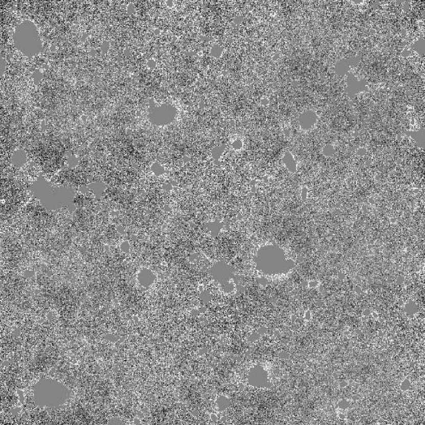
Figure 4: A portion of the NUDF F160W image with the flux level in the source positions set to zero. The image is a linear stretch between $7.5\times 10^{-4}$ and $-7.5\times 10^{-4}$ ADUs per second which corresponds to $2.9\times 10^{-12}$ nW m^-2 sr^-1. There is still some residual flux at the edges of the source removal and from sources below the extraction limit. At the scale of this figure it is difficult to see most of the source extractions which are in general very small.

We performed a fluctuation analysis on 5 images, i) the NUDF F160W image, ii) the image with the 10 sources brighter than 20 mag AB removed to simulate the source subtracted 2MASS images, iii) the image with all detected sources removed, iv) an image created by drizzeling the first and second epoch median images in exactly the same way as the true images, and v) an image of gaussian noise at the level of the NUDF image noise. The fluctuation analysis procedure is described in detail in Appendix A. The only operation performed on the images before the Fourier transform is to set any small DC level to zero to prevent ringing due to a DC component. Figure 4 shows a small portion the NUDF image with all of the sources removed. The results of the analysis are presented in Figure 2. The error bars shown in the figure are for a Gaussian noise due to large scale structure calculated as

$$\Delta P_{2}=\frac{P_{2}}{\sqrt{N_{k}}}$$ (1)

where $N_{k}$ is the number of k components in the half ring of $\Delta k$ used to define the wavenumber bins in Figure 2. We stress that although Gaussian noise may be appropriate for large scale structure, it is an underestimate of the effects of shot noise. The fluctuation power in the Figure has been adjusted for the small amount of sky blanked by removing the sources.

At the request of the referee we computed the fluctuations in the image with the 10 sources brighter than 20 mag AB removed ignoring the regions along the axes in Fig. 5 that correspond to angles of 26 arcseconds or greater. This removes some of the points at larger wavenumbers as well. The only effect, other than to remove the wavenumbers corresponding to 26 arcseconds or greater, was to lower the point in Fig. 2 corresponding to approximately 18 arcsecond by an amount equal to the height of the diamond symbol.

The median image power spectrum gives an indication of how much the fluctuation spectrum can be affected by power in the median image. Figure 2 shows that at angular scales of 10 arcseconds or greater there can be an influence on the all sources subtracted fluctuation spectrum from the median subtraction. The majority of power from resolved galaxies, however, is at smaller angular scales and any median subtraction effects do not alter the conclusions of this paper. It should be emphasized that our conclusion that we would miss backgrounds that are flat on scales of 100 arcseconds comes from our analysis in § 6.2.2, not from the fluctuation spectrum. We also emphasize again that we are not sensitive to fluctuations from population III stars at the pessimistic levels calculated by Cooray et al. (2004) and only at the levels calculated by Kashlinsky et al. (2004) for objects formed at redshift 10.

The amplitude of the two dimensional power spectrum, $\sqrt{f(u,v)f^{*}(u,v)}$ in the notation of the appendix, of the source subtracted image in Figure 4 is shown in Figure 5. All quadrants are shown although the power spectrum is symmetric about the horizontal axis. The stretch is given in the figure caption. Figure 5 shows that there are no significant artifacts in the NUDF image. The small dots and regions of higher intensity are most likely due to the drizzle procedure used to convert the original NICMOS camera 3 0.2 arc second pixels to the 0.09 arc second pixels used to match the rebinned ACS pixels as described in Thompson et al. (2006). Due to the small area removed by the source subtraction, no correction of the power spectrum for the lost area was made.

The difference between the fluctuation spectrum of the full image and the source subtracted image shows that the NUDF contains a rich spectrum of fluctuations due to the sources in the field. When sources brighter than 20 mag (AB) are removed the fluctuations are reduced, with a similar amplitude and shape to that of Kashlinsky et al. (2002). When we further remove all of the sources detected in the NUDF the fluctuation is reduced to a level similar to that of a Gaussian noise field. This clearly shows that the fluctuations from detected NUDF sources with redshifts between 0 and 7 are fully capable of accounting for the fluctuations observed in the 2MASS images without invoking a new population of sources. The vast majority, if not all, fluctuations are simply due to galaxies fainter than the 2MASS calibration field limit which are, however, easily detected in the NUDF image. It is also relevant to the presence of a NIRBE regardless of the type of objects invoked. It shows that normal sources with a total flux of 7 nW m^-2 sr^-1 reproduce the fluctuations observed in the deep 2MASS calibration images. Sources with a total flux 10 times that amount, distributed similarly as the observed sources, would overproduce the fluctuations.

As shown in the work of Cooray et al. (2004) the present fluctuation analysis is not sensitive enough to measure the fluctuations expected from a pessimistic assumption on the expected fluctuations from population III sources. The difference between the pessimistic and optimistic assumptions is 5 orders of magnitude in power and 2.5 orders of magnitude in fluctuations. A comparison with the predictions in Kashlinsky et al. (2004) is presented in § 6. It is inconsistent, however, with high redshift sources of any kind that provide the same flux as ascribed to the NIRBE fluxes claimed in Matsumoto et al. (2005) as was investigated by Magliocchetti, Salvaterra & Ferrara (2003). In that work 1/3 of the H band fluctuation power at small angles is due to population III sources which is clearly not the case in Figure 2 where the all source subtracted fluctuations at an angular scale of 5 arc seconds are factor of 30 below the magnitude 20 source subtracted fluctuations. If the sharp drop in flux between 1.4 $\micron$ and optical flux is interpreted as due to the Lyman limit of high redshift sources then all of the observed flux must be due to such sources. The fluctuation analysis presented here is then evidence against that interpretation.

The NICMOS fluctuations diverge from the noise spectrum at an angular scale of 10″. It is not clear whether the NICMOS fluctuations at these scales are due to faint sources or to other factors such as power in the subtracted median image. It should be noted that the fluctuations are on a scale consistent with small flat fielding errors. We have not attempted to analyze the source subtracted NUDF fluctuations in detail by determining the components due to noise, incomplete flat fielding, median subtraction and faint galaxies. The source subtracted fluctuation amplitudes are therefore only upper limits on fluctuations due to light not coming from the resolved sources. It is also evident from the difference in the fluctuation amplitude for the complete image and the image with the 10 brightest sources removed from the 4700 total sources, that the fluctuation amplitude can vary markedly from field to field, depending on the number of “bright” sources included.

4.1 Fluctuations versus redshift

We next look at contributions to the fluctuations as a function of redshift. To do this we created a series of images which had all sources removed except those in a given redshift range and repeated the analysis. The first redshift range is z =0.0-0.5, with subsequent ranges of width 1 centered on integer redshifts from 1 to 6 and a final range of redshifts above 6.5. The redshifts are photometric redshifts taken from Thompson et al. (2006). As such they are subject to uncertainties but photometric redshifts have been shown to be reliable with occasional catastrophic failures. Most of the redshift ranges contain several hundred galaxies so occasional catastrophic failures should not alter the bulk conclusions. The number of galaxies in each redshift bin is given in Table 2 along with the flux from the galaxies in the bin. Note that although the last bin extends to redshift 10, the limit of the photometric redshift procedure, the detected galaxies are in the redshift range between 6.5 and 7. The fluctuation plots are presented in Figure 6. It is clear that most of the fluctuation power comes from galaxies in the redshift range between 0 and 1.5. By a redshift of 4 the fluctuation power is essentially the same as the all-source-removed fluctuations indicating that the resolved sources at redshifts of 4 and beyond contribute very little to the observed fluctuations.

5 Constraints on Possible Cosmic Near Infrared Backgrounds

The combined NUDF and NHDF fields cover a little over 11 square minutes of sky, in two almost equal areas, in two completely uncorrelated regions of the sky. They contain several thousand objects in areas chosen for a low density of objects. The resolved objects, corrected for missed faint flux, have a maximum total flux of 10 nW m^-2 sr^-1 at 1.1 and 1.6 $\micron$. This is 7 times less than the NIRBE measured by Matsumoto et al. (2005). The NICMOS Hubble deep field observations clearly demonstrate that if a NIRBE exists it can not come from luminous objects that have a spatial distribution of mass and light similar to baryons at redshifts of 6 and less. There is no way to hide 7-10 times the observed flux in the two fields in spatially resolved objects. Any source of a unresolved background over the observed power in galaxies or stars must either be flat or clustered. A flat source of background, not coming from the zodiacal light, will be removed by our median subtraction. If the source of a background is clustered, the two deep fields may have missed observing them. The objects causing the NIRBE would have to be clustered in a manner that the average space between them is more than 2 to 3 arc minutes, but in a way that, while emitting 7-10 times the power of the objects observed in the two deep fields, they avoid detection as resolved objects in the wide field of view DIRBE, NIRS and 2MASS observations.

Our fluctuation analysis of the source subtracted image does not directly rule out an isotropic background. However, within the concordance $\Lambda$CDM model, high redshift galaxies will be clustered, and their emission will show angular anisotropies. Limber’s equation (Limber, 1953) allows one to predict the angular clustering of sources from the spatial power spectrum. The linear power spectrum with a scale independent bias is a conservative lower limit on the fluctuations, and at high redshift it is not a bad estimate. With the 3-d power spectrum, the Limber projection is standard (Baugh & Efstathiou, 1994). Neglecting curved sky effects (which are very negligible here) and assuming a flat cosmology, one has

$$P_{2}(K)=I_{NIRB}\int{dr\over r^{2}}P_{3}(K/r)f^{2}(r)$$ (2)

where $K$ is the wavenumber (aka, $\ell$), $r$ is the comoving coordinate distance (i.e. $\int(c/H)dz$), $I_{NIRB}$ is the average celestial Near Infrared Background of 7 nW m^-2 sr^-1 and $f(r)$ is the distribution of the sources as a function of $r$, normalized to unit integral. $P_{3}(k)$ is the spatial power spectrum in comoving coordinates, normalized as described in the following paragraph. At high redshift, the slices are reasonably thin in $r$ compared to the distance out to that redshift, so one can approximate $r$ as slowly varying over the integral of $f^{2}$. For a uniform distribution of sources between two redshifts, the integral of $f^{2}$ is simply $1/\Delta r$, where $\Delta r$ is the thickness of the slab in $r$. More peaked distributions would give larger answers, increasing the angular correlations. Hence, our lower bound on $P_{2}(K)/I^{2}_{NIRB}$ is $P_{3}(K/r)/r^{2}\Delta r$.

We parameterize the amplitude of the linear power spectrum by $\sigma_{8,flux}$, which is the rms fluctuation of the emissivity in 8h^-1 comoving Mpc radius spheres for the redshift in question. This value is also the $\sigma_{8}$ for galaxies if one weights the galaxies by their luminosity. With this, we find that the rms fluctuations, $\mathcal{F}_{K}$ in Appendix A, at $2\pi/K=10^{\prime\prime}$ scale are $0.1I_{NIRB}\sigma_{8,flux}$ for a screen of sources between redshifts 10 and 14. In other words, for $\sigma_{flux,8}=1$, we predict that the power at $10\arcsec$ scale is $10\%$ of the angle averaged level of the background, if that background is generated at $10<z<14$. The fluctuations scale as the square root of the thickness of the slab; increasing the range to $6<z<20$ only halves the rms fluctuations. Shot noise or non-linear structure formation would increase the clustering above the lower limit set by the linear power spectrum. While we are quoting our amplitude by the familiar $\sigma_{8}$, the scales probed by these data are closer to 0.3Mpc and the linear matter power spectrum is used to make the extrapolation. Small scale filtering by the IGM could cause the smal scale fluctuations to be less than the linear prediction.

The ratio of our observed $10\arcsec$-scale fluctuations to the DC NIRBE level of Matsumoto et al. (2005) is only about $0.7\%$ rather than the $10\%$ found above. To be consistent with the entire NIRBE being due to high-redshift sources the sources would have to be surprisingly unclustered ($\sigma_{8,flux}\lesssim 0.1$ even with shot noise) or the emission must be scattered to smooth out fluctuations on $10\arcsec$ scales, e.g., by scattering of Lyman $\alpha$ into halos much larger than $10\arcsec$. The emission-weighted bias of the undiscovered high redshift galaxies is of course not known, but known populations of high-redshift galaxies are highly clustered (Adelberger et al. (2005), Coil (2004)) and the rare density peaks that form luminous very high redshift proto-galaxies are expected to be highly biased.

Generating the background in thicker slabs at lower redshift can produce smaller fractional fluctuations, as there is more dilution along the line of sight. However, it is implausible that there would be 10 times more emission at low redshift than the sources we already detect, given the extreme depth of the NUDF data and the budget of normal stars in the local Universe. In other words, barring significant scattering, the low level of our observed fluctuations place an upper limit of roughly $10/\sigma_{8,flux}$ nW m^-2 sr^-1 on the flux from high redshift objects (for the $6<z<20$ assumption). Of course, the value can be lower if the observed level is due to noise (as is probably the case), instrumental effects, or the clustering of incompletely removed low-redshift sources.

6 Constraints on a Population III NIRBE

As discussed in the introduction, redshifted light from population III stars has been the topic of several theoretical investigations into the possible origin of a NIRBE. At the proposed redshifts these objects will appear in the NICMOS F160W band but not the F110W and be labeled as F110W dropouts. The total number of F110W dropouts in the NUDF is 3 or less (Bouwens et al., 2005). Note that a detection in a single band can not distinguish high redshift objects from extremely red objects. We will divide our constraints on population III into fluctuation constraints and direct flux constraints.

6.1 Fluctuation Constraints

Predictions of the fluctuations from population III objects have been made by Magliocchetti, Salvaterra & Ferrara (2003), Kashlinsky et al. (2004) and Cooray et al. (2004). Magliocchetti, Salvaterra & Ferrara (2003) ascribe all of the fluctuations observed in the $1.25\micron$ 2MASS deep calibration images after source subtraction to population III objects which is reduced to 1/3 at $1.6\micron$. As mentioned previously our fluctuation analysis of the source subtracted NUDF images produces an upper limit on fluctuations at the 5 arc second scale that is 1/30 of the 2MASS fluctuations, inconsistent with the Magliocchetti, Salvaterra & Ferrara (2003) prediction. We next consider the predictions of Kashlinsky et al. (2004) using the z formation of 10 models from Figure 5 of the paper. In this work only 45 nw m^-2 sr^-1 are ascribed to CIB flux at $1.25\micron$ and the fluctuations at a scale of 5 arc seconds are about 5 nw m^-2 sr^-1. Following Magliocchetti, Salvaterra & Ferrara (2003) we assume that the fluctuations at $1.6\micron$ will be 1/3 that or 1 to 2 nw m^-2 sr^-1. The observed NUDF fluctuations at 5 arc seconds are 1 nw m^-2 sr^-1, consistent with the prediction, particularly given possible variation in fluctuation power in different small fields. The power predictions from Cooray et al. (2004) vary over 5 orders of magnitude in power and 2.5 orders of magnitude in fluctuations depending on the assumptions. The vast majority of that space is far below the sensitivity limit of these observations. In all of the predictions the primary population III fluctuation power is at larger angular scales where the galaxy fluctuation power should be significantly less. The bottom line is that any contribution from population III stars must have a fluctuation power at small angular scales that is equal to or less than the fluctuation power of the all sources subtracted angular distribution shown in Figure 2.

6.2 Direct Flux Constraints

In the following we consider two types of population III emission; point or resolved emission and diffuse emission from scattered Ly $\alpha$ photons.

6.2.1 Point or Resolved population III Sources

Our fluctuation analysis clearly shows that you can not distribute 10 times the flux of the detected objects in additional objects similar to the detected galaxies. At $1.6\micron$ Magliocchetti, Salvaterra & Ferrara (2003) calculate that 1/3 of the observed 2MASS fluctuations are contributed by population III objects. At an angular scale of 5 arc seconds the all source subtracted fluctuations are a factor of 30 below the 2MASS fluctuations and a factor of 100 below the observed NUDF fluctuations from all of the sources. We will, nevertheless, consider the detectability of individual population III galaxies as discussed in the literature. As mentioned in the introduction, Salvaterra & Ferrara (2005) calculate the flux from a $10^{6}$ M_☉ cluster of population III stars at a redshift of 10 and find a spectral peak at 1.6 $\micron$ of 60 nJy with an average of 40 nJy in the F160W band. Figure 3 indicates that the NUDF is complete up to sources of 25 nJy so any such source is easily detectable in the NUDF F160W image. They further calculate that to produce the published NIRBE each NUDF sized region would contain 1165 sources (under the assumption of H cooling) to 5634 sources (under the assumption of H₂ cooling). This far exceeds the observed number of 3 or fewer. Even if the sources are more realistically arranged in a distribution of masses there should be far more detections than observed unless the upper mass limit on the population III stars in the clusters is a few times $10^{5}$ M_☉. This calculation, however, assumes that the emitted light is distributed in the same manner as the mass.

6.2.2 Flux from Diffuse Ly$\alpha$ Emission

Even if the proposed Pop III stars are spatially distributed in a manner similar to lower redshift stars, their light may be differently distributed. Most of the photons from a massive, hot Pop III star are emitted beyond the Lyman limit and converted into Ly$\alpha$ photons that are extensively scattered by the surrounding neutral gas (Loeb & Rybicki, 1999). Most of the background power is then emitted in a diffuse area surrounding the star. Galaxies made up of these stars would have apparent angular sizes between 10 and 100 arc seconds (Kobayashi, Kamaya, & Yonehara, 2006). To test our sensitivity to a diffuse emission, still spatially distributed similar to baryons at lower redshift, we created a simulated image of diffuse emission. The initial image placed diffuse emission in a Gaussian shape with FWHM = $10\arcsec$ at the location of every detected object in the NUDF image. The photon flux of each object was multiplied by 10 to account for the published NIRBE. The simulated image was reflected about both the x and y axis to produce a “random” object field. The diffuse NIRBE image was then added to the original field to see if the simulated NIRBE was detectable. The simulated NIRBE was easily detectable as diffuse but resolved objects, particularly due to the small number of NIRBE sources from bright objects that stood out as intense diffuse objects.

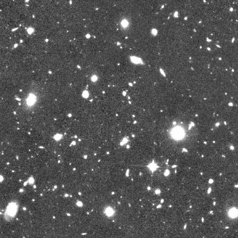
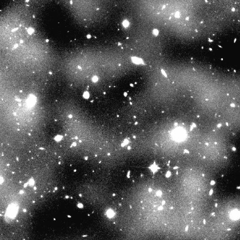
Figure 7: a) A portion of the NUDF F160W image without the addition of a simulated background. b) The same portion of the image with the addition of diffuse background sources represented by Gaussian images with a FWHM of $10\arcsec$. All sources have equal flux and the total background flux is 10 times the flux in detected objects.

The probability of any high redshift object being 10 times as bright as the brightest object in our field is exceedingly remote. The most efficient way to hide the flux from detection is to distribute it equally among all of the objects. A second image was created with all of the objects having equal flux with a total flux equal to the published NIRBE. The median was subtracted from this field as would happen in our reduction and the simulated NIRBE again added to the observed image. The results are shown in Figure 7 where the images with and without the NIRBE are compared. Again the NIRBE sources are easily detectable as enhanced areas of emission. Finally the procedure was repeated using Gaussian sources with a FWHM = $100\arcsec$ which is nearly the size of the image. As would be expected this case produced a very uniform NIRBE which is subtracted out during the median subtraction routine and would have been attributed to zodiacal light in our image processing procedures. If, however, the constraint of exactly equal flux for all objects is lifted, the NIRBE flux is again detectable. These tests indicate that the only way a NIRBE at the flux levels indicated by Matsumoto et al. (2005) could be not detected by our observations is if it is flat on the scale of $100\arcsec$ or larger or if it is clumped on the scale of several arc minutes and our two fields missed the objects contributing to the NIRBE.

7 Conclusions

A fluctuation analysis of the NUDF clearly shows that the fluctuation power found in the 2MASS fields by Kashlinsky et al. (2002) is easily provided by sources with redshifts less than 7 that are below the 2MASS detection limit but easily detectable in the much higher signal to noise NUDF image. There is no need to invoke a high density of population III stars at high redshift to account for the observations. In fact most of the power in the fluctuations comes from low redshift rather than high redshift sources. More important it also shows that sources with a total flux 7 to 10 times less than the flux attributed to the NIRBE produce fluctuations equal to the fluctuations observed in the deep 2MASS calibration images. Sources with fluxes equal to that attributed to the NIRBE, spatially distributed in the same way as the resolved galaxies would overproduce fluctuations by a factor of 7 to 10. The residual fluctuations after source subtraction put a reasonable upper limit of $10\sigma_{flux,8}$ nW m^-2 sr^-1 on any unresolved background component spatially distributed in a manor similar to the observed baryons in the universe. It may be possible to flatten the emission component if it is essentially all Lyman $\alpha$ emission that is scattered over $100\arcsec$ or more but the analysis presented here indicates that there is no observational or theoretical evidence that requires such a component.

In regard to the NIRBE observed by Matsumoto et al. (2005), two of the deepest images ever observed at 1.1 and 1.6 $\micron$ fail by a factor of 7-10 to find resolved objects capable of providing the flux levels of the published 1.4 - 1.8$\micron$ NIRBE. Although the absolute power observed by NICMOS and NIRS are consistent, the distribution of that power between a flat component and resolved sources differs. The very high resolution NICMOS images differentiate the two components by direct observation, unambiguously separating the resolved component from the flat component. The separation in the NIRS observations is accomplished with models for both the zodiacal light and the stellar and galaxy population. The amount of flux attributed to the zodiacal light by the model used in the NIRS observations is significantly less than the flat background found in the NICMOS observations and the difference is of the same order of magnitude as the NIRBE. This leads to the possibility that the flux attributed to the NIRBE by Matsumoto et al. (2005) is simply residual zodiacal light unaccounted for by the model. This is reinforced by the observation by Dwek, Arendt & Krennrich (2005) that the spectrum of the NIRBE found by Matsumoto et al. (2005) is very similar to the spectrum of zodiacal light, as was also noticed by Matsumoto et al. (2005). Since the high z population III light should have a similar spectrum this is not definitive evidence for a zodiacal interpretation but it does indicate that the data is consistent with a zodiacal interpretation.

These observations, coupled with the theoretical implications of the published NIRBE discussed in § 1.2 lead us to the conclusion that the NIRBE does not exist and arose from an incomplete subtraction of the zodiacal light. An important caveat to this conclusion is that the two deep NICMOS field cover an extremely small area of sky. This means that any NIRBE that is flat such as might be produced by widely scattered Ly $\alpha$ emission, or is clumped, as perhaps population III stars might be, will either be subtracted from or missed by the NICMOS deep fields. These caveats, however, do not dismiss the theoretical objections to the NIRBE.

Appendix A Calculation of Fluctuations in the NUDF

In order to compare our observations with the fluctuations observed in the 2MASS images by Kashlinsky et al. (2002) we performed a fluctuation analysis on the NUDF F160W image. Due to the small scale flat field residuals described in § 2.1 we did not perform a similar analysis on the F110W image. The purpose of this appendix is to give an exact description of the analysis method so that it can be repeated on the NUDF Treasury images in the HST archive. For ease in performing the Fourier transforms, the mosaic image in its camera oriented rectangular format was used rather than the rotated version with north up.

A.1 Source Removal

All pixels identified by SE as part of a source are set to 0 for the source subtracted image and only those from sources brighter that 20 AB mag for the comparison image to the previously analyzed 2MASS images. The procedure for identifying those pixels is described in § 2.2. Next the weight image from the Version 2 NUDF Treasury submission was divided by its median to produce a normalized weight image. The source subtracted image was then multiplied by the normalized weight image. After this step the median of the image was subtracted from the image to remove any remaining residual DC component before performing a 2 dimensional Fourier Transform. No further processing was done on the image.

A.2 Fluctuation Analysis

The fluctuation analysis follows the prescription for analysis of fluctuations in the temperature of the CMB presented in Peacock (1999). The original image which is in ADUs per second is converted to Watts m^-2 Hz^-1 per pixel by the standard conversions for the NICMOS instrument. The flux is then multiplied by the frequency of 1.6 $\micron$ and divided by the solid angle in steradians subtended by a single pixel to produce a new image in units of Watts m^-2 Sr^-1 which is designated $F(\vec{\theta})$ where $\vec{\theta}$ is the angular distance from the lower left corner of the image in radians. We then take the Fourier transform of the image defined as

$$f_{K}(\vec{K})=\frac{1}{L^{2}}\int F(\theta)e^{-\vec{K}\cdot\vec{\theta}}d^{2}\theta$$ (A1)

where $L$ is the angular dimension of the square image and $\vec{K}$ is the wave number. The square of the fluctuation for wave number $\vec{K}$ is given by

$$\mathcal{F}^{2}_{K}=\frac{L^{2}}{(2\pi)^{2}}2\pi K^{2}\mid f_{K}\mid^{2}$$ (A2)

If $\vec{K}$ is in units of inverse radians, then it is equivalent to the multipole degree $l$ and

$$\mathcal{F}^{2}_{K}=\frac{l^{2}}{2\pi}C_{l}$$ (A3)

A.3 Translation into Fourier Series

Although equations A1 and A2 provide elegant definitions for the fluctuation, the actual calculations involve digital Fourier series rather than integrals. We used the IDL Fourier series procedure in this analysis so we will use that definition in this appendix. The IDL forward Fourier series is defined by

$$f(u,v)=\frac{1}{N^{2}}\sum_{x=0}^{x=N-1}\sum_{y=0}^{y=N-1}F(x,y)e^{\frac{-2\pi iux}{N}}e^{\frac{-2\pi ivy}{N}}$$ (A4)

The returned wave numbers are given by

$$u_{i}=\frac{i}{N\delta\theta}$$ (A5)

where $\delta\theta$ is the pixel spacing in radians. Comparing equation A1 with equation A4 we note that $L=N\delta\theta$ and that $d^{2}\theta=\delta\theta^{2}$ giving the $\frac{1}{N^{2}}$ term in the IDL Fourier Series. We also note that the components of $\vec{K}$ in the x and y directions are $2\pi u$ and $2\pi v$.

The Fourier series returns a 2 dimensional array of the same size as the image which is aliased around its midpoint so that we only consider wave numbers in a semicircle in either the upper or lower half of Figure 5. We calculate the wave number for each point in the returned array and take the amplitude of the Fourier series at that point. We next establish a log spaced vector of $K$ values and find the average, $\mid f_{K}\mid$, of the $f_{K}$ values in the bins defined by the $K$ vector to calculate the fluctuation given by the square root of equation A2. Figure 2 is the plot of those values versus angle where the angle is $\frac{2\pi}{K}$ and radians are converted to arc seconds. To assess the influence of the weight image a similar analysis was done without multiplication by the weight image. The only amplitude with a visible change on the scale of Figure 2 was the very last point.

Table 1: Measured Background Fluxes

Measurement	Total Flux	Zodiacal Flux	Detected or expected sources	Residual Flux
NUDF 1.6 $\micron$	461.9	455.0	$6.9^{+3.}_{-0.3}$	$0.0^{+3.}_{-0.3}$
NUDF 1.1 $\micron$	350.5	342.20	$6.3^{+3.}_{-0.3}$	$0.0^{+3.}_{-0.3}$
NHDF 1.6 $\micron$	327	320	$7.0^{+3.}_{-0.3}$	$0.0^{+3.}_{-0.3}$
NHDF 1.1 $\micron$	341	334	$7.0^{+3.}_{-0.3}$	$0.0^{+3.}_{-0.3}$
NIRS 1.63 $\micron$	320.0	224.0	30.1	65.9
NIRS 1.43 $\micron$	332.1	230.0	32.1	70.1

Table 2: Number of galaxies in each redshift bin

Redshift Range	0.0-0.5	0.5-1.5	1.5-2.5	2.5-3.5	3.5-4.5	4.5-5.5	5.5-6.5	6.5-10.0
Number of galaxies	511	1520	931	930	513	218	64	13
Flux in nW m-2 sr-1	2.8	3.3	0.32	0.39	0.087	0.014	0.0046	0.00003

Figure 1: Plot of the NIRBE flux from Matsumoto et al. (2005) shown as asterisks. The squares are object fluxes from Madau & Pozzetti (2000), the triangles are the NUDF object fluxes from Thompson et al. (2006), the plus signs are those fluxes corrected for the expected missing flux from faint galaxies and regions of galaxies and the diamonds are the quoted backgrounds from Kashlinsky (2005a). The crosses with error bars are the DIRBE fluxes from the references in table 3 of Kashlinsky (2005a) plus the 1.25$\micron$ point from Wright (2001). Only claimed detections are plotted rather than upper limits.

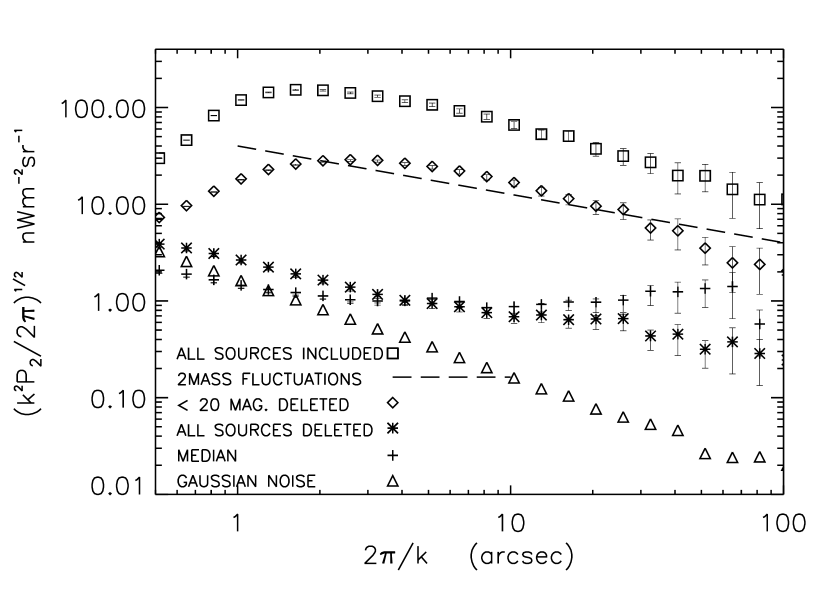
Figure 2: The fluctuation spectrum of the of the F160W NUDF image is given by the squares, the image with sources brighter than 20 AB mag. subtracted by the diamonds, with all sources subtracted by the asterisks, and the fluctuations of a Gaussian noise field by the plus signs. The dashed line represents an average of the fluctuations found by Kashlinsky et al. (2002) in 7 different 2MASS calibration fields. The photon Poisson noise for the all sources included and brighter than 20. mag deleted curves is smaller than the symbol sizes. The error bars give the Gaussian noise as described in the text.

Figure 3: a) The left hand figure shows the histogram of the number of pixels in detected sources having a given flux in nJy in the F160W NUDF image. The dashed line with slope -1 is not a least squares fit to the data. b) The right hand figure plots the number of sources for a given total source flux. The dashed line with slope -0.63 is not a least squares fit to the data.

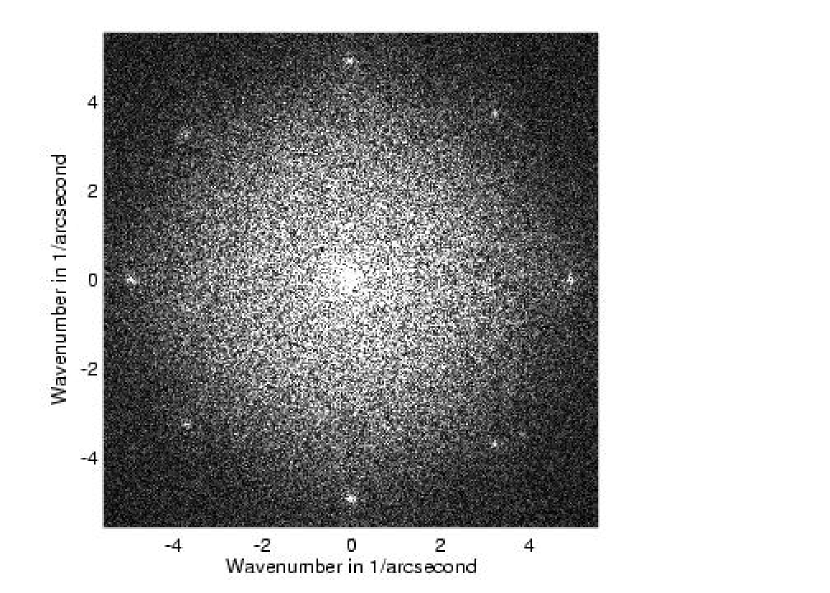
Figure 5: The amplitude of the 2 dimensional power spectrum, $\sqrt{f(uv)f^{*}(u,v)}$ in the notation of the appendix, of the source subtracted image shown in Figure  4. The figure is symmetric around the horizontal axis with a linear stretch between 0 and 1/30 of the maximum value. Other than the white dots in the spectrum, there are no artifacts at the spatial scales relevant to this study. The white dots are most probably due to the effects of the drizzle procedure as discussed in the text.

Figure 6: The fluctuation spectra with all resolved sources removed except the sources in the redshift ranges indicated by the title at the top of each plot. The fluctuation spectra for redshifts of 4 and above are almost identical to the spectrum for all sources removed shown in more detail in Figure 2. Any flux not in resolved sources is retained in all spectra.

References

- Adelberger et al. (2005) Adelberger, K.L, et al. 2005, ApJ, 619, 697
- Aharonian et al. (2006) Aharonian, F. et al. 2006, Nature, 440, 1048
- Baugh & Efstathiou (1994) Baugh, C.M. & Efstathiou, G. 1994, MNRAS, 267,323
- Bertin & Arnouts (1996) Bertin,E., & Arnouts, S. 1996, A&A, 117, 393
- Bouwens et al. (2005) Bouwens, R.J., Illingworth, B.D., Thompson, R.I. & Franx, M. 2005, ApJ, 624, L5
- Cambresy et al. (2001) Cambresy, L., Reach, W. T., Beichman, C. A., & Jarrett, T. H. 2001, ApJ, 555, 563
- Cohen et al. (1997) Cohen, M. 1997 in ASP Conf. Ser. 124, Diffuse Infrared Radiation and the IRTS, ed. H. Okuda, T. Matsumoto, & T. Roelig (San Francisco: ASP), 61
- Coil (2004) Coil, A. L., et al 2004, ApJ, 609 525
- Cooray et al. (2004) Cooray, A., Bock, J.J., Keatin, B., Lange, A.E., & Matsumoto, T. 2004, ApJ, 606, 611
- Dickinson (2000) Dickinson, M. 2000, Phil. Trans. R. Soc. London A., 358, 2001
- Dwek and Arendt (1998) Dwek, E. & Arendt, R. G. 1998, ApJ, 508, L9.