Debris disks in main sequence binary systems

Abstract

We observed 69 A3-F8 main sequence binary star systems using the Multiband Imaging Photometer for Spitzer onboard the Spitzer Space Telescope. We find emission significantly in excess of predicted photospheric flux levels for 9${}^{+4}_{-3}$% and 40${}^{+7}_{-6}$% of these systems at 24 and 70 µm, respectively. Twenty two systems total have excess emission, including four systems that show excess emission at both wavelengths. A very large fraction (nearly 60%) of observed binary systems with small ($<$3 AU) separations have excess thermal emission. We interpret the observed infrared excesses as thermal emission from dust produced by collisions in planetesimal belts. The incidence of debris disks around main sequence A3-F8 binaries is marginally higher than that for single old AFGK stars. Whatever combination of nature (birth conditions of binary systems) and nurture (interactions between the two stars) drives the evolution of debris disks in binary systems, it is clear that planetesimal formation is not inhibited to any great degree.

We model these dust disks through fitting the spectral energy distributions and derive typical dust temperatures in the range 100–200 K and typical fractional luminosities around $10^{-5}$, with both parameters similar to other Spitzer-discovered debris disks. Our calculated dust temperatures suggest that about half the excesses we observe are derived from circumbinary planetesimal belts and around one third of the excesses clearly suggest circumstellar material. Three systems with excesses have dust in dynamically unstable regions, and we discuss possible scenarios for the origin of this short-lived dust.

1 Introduction

The majority of solar-type and earlier main sequence stars in the local galaxy are in multiple (binary or higher) systems (Duquennoy & Mayor, 1991; Fischer & Marcy, 1992; Lada, 2006). Planetary system formation is necessarily more complicated in multiple stellar systems because of more complex dynamical interactions. However, protoplanetary disks are known to exist in pre-main sequence binary systems both from spectral energy distributions (Ghez et al., 1993; Prato et al., 2003; Monin et al., 2006) and from images (Koerner et al., 1993; Stapelfeldt et al., 1998; Guilloteau et al., 1999). Some older binary systems also offer evidence of planetary system formation, with both planets (Patience et al., 2002; Eggenberger et al., 2004; Konacki, 2005; Bakos et al., 2006) and debris disks (Aumann, 1985; Patten & Willson, 1991; Koerner et al., 2000; Prato et al., 2001) known. Planetary system formation — broadly defined — must be common in a significant fraction of multiple stellar systems.

Studying planetary system formation through direct observation of planets orbiting other stars is prohibitively challenging at present. The nearest targets (for which we have the greatest sensitivity) are generally mature, main sequence stars broadly similar to our Sun, where the signatures of planet formation have long since been replaced by processes endemic to mature planetary systems. We must therefore study the properties of planetary systems indirectly. It is generally thought that the formation of planetesimals is a natural byproduct of (advanced) planetary system formation; our Solar System’s asteroid belt and Kuiper Belt are remnant small body populations that reflect the epoch of planet formation. These small bodies, in our Solar System and in others, occasionally collide, producing collisional cascades that ultimately produce dust. Because dust is the most easily observable component of planetary systems due to its relatively large surface area, one avenue to understanding planetary system formation is to study dusty debris disks around other stars. However, no sensitive, systematic examination of the frequency of debris disks — signposts of planetary system formation — in multiple systems has been carried out.

Dust heated by stellar radiation to temperatures of tens to hundreds of Kelvins is best observed at mid- and far-infrared wavelengths, where the contrast ratio between the thermal emission of the dust and the radiation of the star is most favorable. In many cases the dust temperature and fractional luminosity can be measured or constrained from the observations. Under certain assumptions of grain properties (size, albedo, emissivity, size distribution) estimates can be made of the dust mass present and potentially of the properties of the planetesimals that produced the observed dust grains (e.g., Beichman et al., 2005b; Su et al., 2005).

Dust in planetary systems generally must be ephemeral because the timescales for dust removal are short compared to the main sequence ages of the host stars (e.g., Backman & Paresce, 1993). The processes of dust production and removal are more complicated in multiple systems than around single stars, but any dust must nevertheless be regenerated from a source population of colliding bodies. Dust production can either be through a continuous collisional cascade, through stochastic (occasional) collisions, or derived from individual bodies (e.g., sublimation from comets). Ultimately, a relatively substantial population of larger bodies (planetesimals: meter-sized up to planet-sized) is implied under either model of dust production, and argues that planet formation must have proceeded to some degree in every system with dust, and therefore every system with excess thermal emission.

There are extensive programs with the Spitzer Space Telescope to study debris disks around single stars (e.g., Beichman et al., 2005b, a; Rieke et al., 2005; Kim et al., 2005; Bryden et al., 2006; Su et al., 2006), but binaries — a majority of solar-type stars — have generally been explicitly omitted from these surveys. To understand the processes of planetary system formation and evolution in this common hierarchical system we have carried out a Spitzer survey for infrared excesses around 69 binary star systems to look for thermal emission from dust grains. Our primary goal is to address whether the incidence of debris disks in multiple stellar systems is different than that for single stars. Here we present our 24 and 70 µm observations of these 69 systems and identify excess emission from a number of them. We discuss our overall results and individual systems of note, as well as the dynamical stability of dust in binary systems. We conclude with a discussion of the implications of our observations for planet and planetary system formation in binary systems.

2 Sample definition

We observed 69 binary (in some cases, multiple) main sequence star systems in order to study the processes of planetary formation in multiple systems and particularly to search for effects of binary separation on the presence of debris disks. We chose to observe late A through early F stars for reasons of economy: their photospheres are bright and we could thus reach a systematic sensitivity limit for a significant sample in the shortest observing time. The primaries in our sample are 18 A stars (A3 through A9) and 51 F stars (F0 through F8). We have not done an exhaustive study for higher multiplicity (greater than binarity) for the 69 systems in our sample. Our targets were vetted to eliminate high backgrounds, and were chosen independent of whether IRAS data implies any excess for that system. Our target list also excludes systems with extreme flux ratios between the two components, and the secondary is generally G-type or earlier; in practice, this information is available for only one third of our targets.

Our primary goal is to determine whether the incidence of debris disks in binary systems is different than that for single stars. Our secondary goal is to determine whether there is any effect on debris disk properties due to binary separation. Our sample is therefore divided into three subsamples by binary separation to look for possible trends in the frequency of infrared excess (that is, planetary system formation) as a function of binary separation. (In some cases, these separations are the projected separations, not the actual orbital distance.) 21 targets in this program have separations less than 3 AU; 23 systems have separations of 3–50 AU; and 19 systems have separations of 50–500 AU. Our sample also includes 6 systems with very large separations ($>$500 AU). We present results for this last group in this paper, but do not include them in our analysis of excess as a function of binary separation.

Typical distances to our targets are 20–100 pc, though a couple of systems are as close as 12 pc. The angular resolution of Spitzer 24 µm observations is 6″ (and 18″ at 70 µm), and almost all of our systems have angular separations smaller than this and are therefore unresolved at both Spitzer wavelengths. A handful of systems are resolved (in some cases barely) at one or both Spitzer wavelengths. Our photometric treatment of both resolved and unresolved systems is discussed in Sections 3.1 and 4.1.

The physical properties of these systems — including (projected) binary separation and age, both of which may have an effect on the rate of occurrence of debris disks — are reported in Table 1. Appendix A gives details of our derivations of stellar properties for this sample.

3 Observations and data reduction

3.1 Spitzer observations

A listing of the observations for this program (Spitzer PID #54) is given in Table 2. All Spitzer observations were made between January, 2004, and March, 2005. We used the Multiband Imaging Photometer for Spitzer (MIPS; Rieke et al., 2004) to make observations of each system at 24 µm and, for most systems, 70 µm (effective wavelengths 23.68 and 71.42 µm, respectively). All stars were observed using the MIPS Photometry observing template in small-field mode. The 24 µm observations were all made using 3 sec DCEs (data collection events) and a single template cycle. The 70 µm observations typically used 10 sec DCEs and 5 to 10 template cycles.

Data were processed using the MIPS instrument team Data Analysis Tool (Gordon et al., 2005). For the 24 µm data basic processing included slope fitting, flat-fielding, and corrections for droop and readout offset (jailbar). Additional corrections were made to remove the effects of scattered light (which can introduce a gradient in the images and an offset in brightness that depends on scan-mirror position), and the application of a second order flat, derived from the data itself, to correct latents that were present in some of the observations. The 70 µm data processing was basically identical to that of the Spitzer pipeline (version S13). Mosaics were constructed using pixels 1$\farcs$245 and 4$\farcs$925 square at 24 and 70 µm, respectively (about 1/2 the native pixel scale of those arrays).

We used aperture photometry to measure the fluxes from our target systems. Aperture corrections were computed using smoothed STinyTim model PSFs (Krist, 2002) for a 7000 K blackbody source. The model PSFs were smoothed until they provided good agreement with observed stellar PSFs, as described in Gordon et al. (2006) and Engelbracht et al. (2006).

The PSF full width at half maximum at 24 and 70 µm is 6$\farcs$4 and 19$\farcs$3, respectively. Systems with angular separations less than 6″ are unresolved at both MIPS wavelengths. For these targets, fluxes were measured using relatively small apertures of 9$\farcs$96 and 39$\farcs$4 in diameter (at 24 and 70 µm, respectively) to improve the signal-to-noise ratio (SNR) of the measurements. (In a few cases at 24 µm nearby sources contributed some flux at the target location, so we used apertures 25% smaller than those just described to reduce contamination.) Systems with angular separations between 6″ and 30″ are resolved at 24 µm but not at 70 µm. For these cases, we used apertures 35″ in radius to measure the system-integrated flux. Where the components were visible and clearly separated (at 24 µm), we compared the photometry from the large aperture with the sum of the fluxes from the individual components (measured using the smaller apertures) as a cross check. Five systems have large enough angular separations ($>$30″) that they are resolved not only at 24 µm but also at 70 µm: HD 142908, HD 61497, HD 77190, HD 196885, and HD 111066. For these five systems, only photometry for the primary is measured, modeled, and reported; we have no measurements for the companions through either being too faint or out of the field of view.

The photometric aperture was centered at the center-of-light of each target except in cases where the 70 µm detection was weak or there was cirrus or background contamination, where we forced the aperture to be centered at the target coordinates. The fluxes we report are based on conversion factors of 1.048 $\mu$Jy/arcsec²/(DN/s) and 16.5 mJy/arcsec²/U70 at 24 and 70 µm, equal to the calibration in the Spitzer Science Center pipeline version S13 (further details on calibration can be found in Rieke et al. (2006), Gordon et al. (2006), and Engelbracht et al. (2006)).

The 24 and 70 µm Spitzer photometry for all sources observed in this program is reported in Table 3, together with the system-integrated V and K band magnitudes used in photospheric model fitting (Section 4.1). All targets were strongly detected at 24 µm, with intrinsic S/N in the hundreds to thousands. The 70 µm observations were planned such that the predicted combined photospheric flux from the system could be detected with S/N of at least 3 in 1000 second; the 16 systems that did not meet this criterion were not observed at 70 µm. We also discard from our statistical sample the three sources that were observed at 70 µm but not detected, leaving 50 good observations at 70 µm.

All measurements are subject to both photometric (measurement) error and a uniform calibration uncertainty of 4% at 24 µm and 8% at 70 µm (Gordon et al., 2006; Engelbracht et al., 2006). These two sources of error are RSS-combined to calculate the total errors presented in Table 3.

3.2 Submillimeter observations

We observed 13 of our systems at 870 µm with the Heinrich Hertz Submillimeter Telescope on Mt. Graham, Arizona. The data were reduced using the NIC package, which produces mosaicked images from the 19-channels of the detector, subtracts the “off” images from the “on,” and accounts for atmospheric opacity (which we measured regularly using sky-dips). Flux calibrations were derived from observations of the planets (primarily Neptune and Mars). The typical 3-sigma sensitivity achieved in those observations was $\sim$30 mJy. None of the 13 systems were detected above the 3-sigma level, and upper limits for each system are given in Table 3. Our submillimeter observing program was cut short due to the failure of the facility bolometer array, and the remaining systems have not been observed by us in the submillimeter.

Assuming an excess temperature of 50 K, the “minimum temperature fit” that we employ below and which gives the maximum submillimeter flux, the ratio of 70 µm flux to 870 µm flux is $\sim$12, so the 70 µm flux ideally would have to be greater than $\sim$350 mJy for us to have made a significant detection in the submillimeter. HD 13161 is the only target in our sample with a 70 µm flux greater than 150 mJy. Since this target unfortunately was not observed before the demise of the bolometer array, it is not surprising that all of our 870 µm observations are upper limits.

For all 13 sources observed at 870 µm the upper limits do not significantly constrain the debris disk models that we present in this paper.

4 Results

4.1 Modeling photospheric fluxes

From published visible and near-infrared data, we determine the best-fit Kurucz model spectrum; details of this process are described in Appendix A. Many of our systems are resolved in visible and near-infrared data, but almost all are unresolved at one or both Spitzer wavelengths (Section 3.1). Our approach is therefore to combine fluxes at any wavelength where the components are resolved into a single system-integrated flux measurement (with the five exceptions listed in Section 3.1 and Table 3).

We model the combined flux from each binary system as a single stellar source. This approach is satisfactory regardless of the (dis)similarity between the two spectral types: for every primary star presented here, no secondary spectral type changes the the slope of the Rayleigh-Jeans part of the spectral energy distribution (SED) by more than 1% from the trivial case of primary and secondary stars having identical spectral types. The errors in our predictions are therefore always small compared to other sources of error.

Using the best-fit Kurucz model, we predict the fluxes for the Spitzer observations at the 24 and 70 µm effective wavelengths. These predicted photospheric fluxes are listed in Table 3.

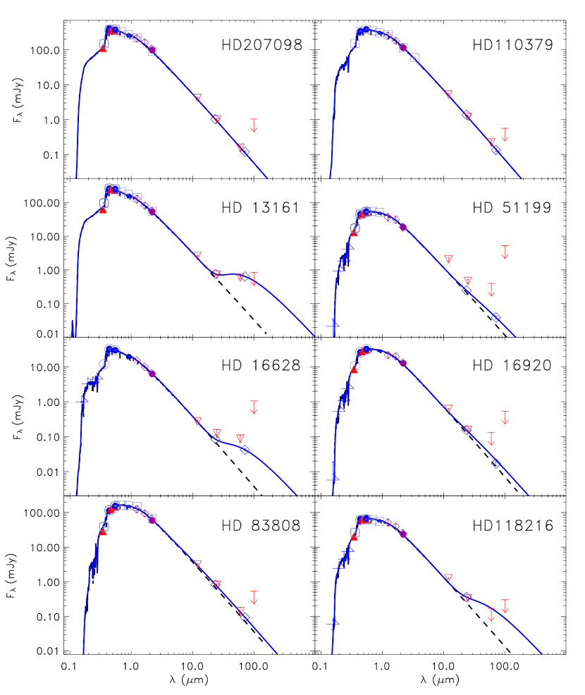
Figure 1: Spectral energy distributions (SEDs) for eight binary systems. The top two panels show systems that have no excess emission at either Spitzer wavelength, whereas the remaining six panels show SEDs for systems with various kinds of excesses, as described in Section 5.3. In all cases, the blue solid line shows our best-fit SED, and the dashed black line is the best-fit scaled Kurucz model spectrum that is our modeled photospheric flux. The Kurucz model is fit to the combined flux of the two stars, using optical and near infrared data: 2MASS data is shown as purple diamonds, with “super-K” (see Table 3) as a filled purple circle, and various other ground-based visible datasets (see Appendix A) are shown. Our Spitzer/MIPS measurements are shown as blue diamonds, with IRAS data points are shown as red downward pointing triangles (or upper limits). In some cases, IRAS fluxes are significantly above our best-fit SED due to flux from other (non-targeted) sources in the IRAS beam that are excluded by our aperture photometry. Since IRAS data is not used in determining the best Kurucz model or the best-fit SED, these discrepancies do not affect our analysis or interpretation. The top two panels demonstrate that our 24 and 70 µm photospheric predictions generally correspond quite well to predicted fluxes for systems with no excesses. Details of the best-fit disk models are presented in the text and in Table 4. Fractional luminosity is the ratio of the total emission from the disk to the total emission from the star(s). For HD 13161, HD 51199, HD 16628, and HD 83808, the SEDs shown here correspond to the debris disk solutions given in Table 4. For HD 118216, we show here an SED that corresponds to a dust temperature of 134 K (see Section 5.3). For HD 16920, we show here an SED that corresponds to a dust temperature of 260 K (Section 5.3).

In Figure 1 we show SEDs for two binary systems with no excess emission in our MIPS observations. These systems are representative of our method of photosphere modeling and predicting 24 and 70 µm photometry. The measured Spitzer photometry falls quite close to the predicted fluxes in all cases. It is clear that our technique of fitting a single temperature model works quite satisfactorily both in the visible/near-infrared and also at Spitzer wavelengths.

4.2 Determination of excesses

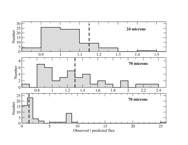
Figure 2: Histogram showing R24 (upper) and R70 (middle and lower), where R is the ratio of observed flux to predicted flux. The middle and lower panels show the same data, but with different bin sizes and horizontal scales in order to show both the inner core (R70 near unity; middle panel) and the total range of R70 (lower panel). (Some R70 values low and high are beyond the compressed range of the middle panel but appear in the bottom panel.) There are 69 systems with 24 µm measurements and 50 systems with 70 µm measurements. The excess threshold values of 1.15 (24 µm) and 1.30 (70 µm) are indicated with dashed lines.

We use the ratio (R) of observed flux (F) to predicted flux (P) to determine the excess threshold and to identify excess emission. In Figure 2 we show histograms of R24 and R70 for all observed systems. The R24 distribution is well fit by a gaussian centered at R24 = 0.99 and $\sigma=0.05$. We take a conservative approach, adopting an excess threshold ratio of 1.15 (Figure 2, top), which formally is slightly more than 3-sigma. The R24 dispersion less than unity, which should represent excursions $\lesssim$3$\sigma$, extends smoothly down to 0.85, confirming $\sigma=0.05$.

It is more difficult to produce a well-fit gaussian to the 70 µm data because there are only 50 measurements (fewer than at 24 µm), of which more than one third likely have excesses (Figure 2, middle). The scatter in the R70 distribution implies $\sigma=0.10$, centered near unity, suggesting that we adopt a 3-sigma error threshold of 1.30. We note that both the R24 and R70 excess thresholds are consistent with, though perhaps somewhat larger than, the errors due to systematic calibration uncertainties, giving us confidence that our thresholds are accurate but also conservative.

In most cases, our observed 24 and 70 µm fluxes are within 1 sigma (5% and 10%, respectively) of the predictions (Table 3), confirming that our photospheric predictions are good. Occasionally the measured fluxes are less than the predictions by 2–3 sigma, and a number of cases have observed fluxes that are greater — in some cases, substantially so — than the predictions. Some of these individual cases with significant excesses are discussed in Section 5.3. We note, however, that one 24 µm and three 70 µm measurements have R values that deviate from unity by more than 3$\sigma$ (Table 3). The existence of these low R24 and R70 values may indicate that we have underestimated the scatter in the data, as we would expect no values more than 3$\sigma$ below unity for a sample of this size. This may in turn imply that a few systems that we identify as excesses based on their R values may be spurious (noise rather than true excesses). For this reason, we introduce the additional requirement of having significant excess emission, as follows.

We calculate the significance ($\chi$) of a detected excess as

$$\chi=\frac{F-P}{\sigma}$$

where F and P are as defined above and $\sigma$ is the total error (photometric error [noise] and calibration error, added in quadrature) of the measurement. This figure of merit $\chi$ is calculated for each measurement at each wavelength (Table 3). The significance of a measurement that exactly matches the prediction is zero.

Formally, to identify excess emission from a system, we require that R be greater than the thresholds derived above and that the significance be 2.0 or greater. Thus, systems like HD 8556 are, sensibly, excluded from being valid excess detections (with R70 = 1.35 and $\chi_{70}=1.01$, the “excess” $F-P$ here is comparable to the total error $\sigma$). We list all valid excess systems in Table 4.

4.3 Overall results

Using the criteria explained above, we find that 9${}^{+4}_{-3}$% of the systems have excess emission at 24 µm (6/69) and 40${}^{+7}_{-6}$% show excess at 70 µm (20/50), using binomial errors that include 68% of the probability (equivalent to the 1$\sigma$ range for gaussian errors), as defined in Burgasser et al. (2003). Four systems have excesses at both wavelengths.

Individual 24 µm excesses range from 16% to 47% above the predicted combined photospheric flux (Figure 2, Table 4). R70 ranges from 1.3 to more than 25 (Figure 2, Table 4). A 100% excess above the predicted combined photosphere (that is, R of 2) means that the thermally emitting dust in the system is as bright as the total flux from the star at the specified wavelength. Eleven systems have R70$\geq$2.0. These very large excesses indicate relatively high fractional luminosities, which in turn imply large amounts of dust in these systems.

4.4 Identification of false IRAS excess

Seven sources have IRAS 25 µm fluxes (Moshir et al., 1989) more than 30% above the predicted photosphere: HD 13161, HD 13594, HD 16920, HD 20320, HD 80671, HD 83808, and HD 118216 (considering only quality flag 3 data). One source has a measured IRAS 60 µm flux more than 50% above its predicted photosphere: HD 13161 (again, considering only quality flag 3 data). Except for HD 13594, the IRAS measurements, after color- and wavelength-corrections, are all quite consistent with our Spitzer measurements (Table 3, Table 4) and we confirm the IRAS-detected excesses for these six systems (indeed, as indicated in Section 5.3 and Appendix B, several systems were identified as excess systems previously based on the IRAS data). In contrast, the color-corrected IRAS 25 µm measurement for HD 13594 is 50% higher than our 24 µm measurement, and two sigma above the predicted photospheric flux at 25 µm (using the IRAS reported error). We see no additional sources in our 24 µm image of this target; contamination in the large IRAS beam is probably not the explanation for the high 25 µm flux. We speculate that the IRAS measurement is simply anomalously high. Since debris disk searches are often still based on catalogs of IRAS-selected excesses, we identify here HD 13594 as a false excess so that future disk searches need not spend time observing this source.

5 Analysis of observational results

5.1 Excess as a function of binary separation

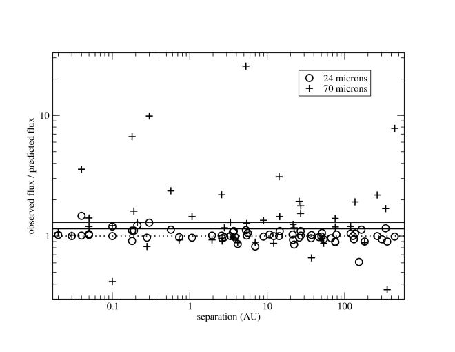
Figure 3: Ratio of observed to predicted fluxes for all systems as a function of binary separation. Circles show data for 24 µm observations and crosses show results for 70 µm observations. In all cases the errors in R24 and R70 are smaller than the symbols. The solid horizontal lines show our criteria for identification of excess at R24 = 1.15 (lower line) and R70 = 1.30 (upper line), and the dotted line shows R = 1.00, for guidance. There is no significant trend with separation, although systems with separations 1–10 AU may have fewer, or smaller, excesses.

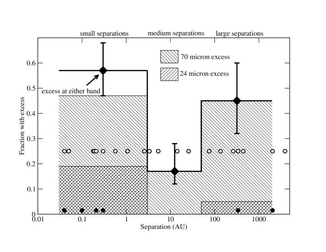
Figure 4: Fraction of binary systems in each of three logarithmic bins (0–3 AU; 3–50 AU; 50–200 AU) that have 24 µm (diagonal pattern lower left to upper right), 70 µm (diagonal pattern lower right to upper left), or 24-or-70 µm excesses (clear). Binomial error bars are shown for the 24-or-70 µm excesses category. Each category reads from the bottom of the plot (that is, the fraction of close binaries with 70 µm excesses is 47%). Some systems have excesses at both wavelengths, and the number of observed systems is not the same at 24 and 70 µm, so the combined fractions do not simply equal the sum of the two subcategories. The separations of the individual systems with excesses contained within each bin are indicated by the filled (24 µm) and open (70 µm) circles (with arbitrary y-axis values). Intermediate separation systems have fewer excesses than small or large separation systems, as expected (Section 6.6).

R24 and R70 as a function of separation are shown for the individual measurements in our sample in Figure 3. The systems with excess are shown in Figure 4. The excess rates for small and large separation systems are around 50%, and there are fewer medium separation systems with excesses than either small or large separation systems. The relative lack of excesses in systems with medium separations confirms our theoretical expectations (see Section 6.6). A smaller excess rate for medium separation systems is also in agreement with observations of pre-main-sequence binaries that suggest that systems with separations 1–50 AU (approximately equal to our medium separation bin) have significantly fainter disks than systems with large separations (Jensen et al., 1994). The significances of high excess rates for small and wide separation binaries, and a low excess rate for medium separation binaries, are discussed in Section 9.1.

5.2 Properties of the dust disks

5.2.1 Dust temperatures

In previous sections we have discussed excess emission detected at 24 and 70 µm. We now move to the astrophysical interpretation of this excess emission as thermal radiation from dust grains heated by the radiation fields of the star(s). We assume these grains are large and model them as blackbodies. (We briefly explore the implications of non-black-body grains in Section 8.2.) We derive best-fit temperatures for these dust grains, assuming a single temperature for the ensemble population, based on a uniform distance from a single radiation source. While the radiation and temperature fields in binary systems are certainly more complicated than these simple assumptions, in general the results of these approximations will be adequate to help us understand the properties of the systems we observe and allow comparisons among the systems presented here, and to results presented elsewhere.

To calculate dust temperatures for systems with excesses, we used the following techniques. For systems with both 24 and 70 µm excesses (four systems), we fit a blackbody to the excess emission in both bands. For systems with only a 70 µm excess, we fit the 70 µm excess emission and the 3-sigma upper limit on the 24 µm emission (that is, the predicted flux plus three times the 1-sigma error bar). This approach produces an upper limit to the excess temperature (and dust luminosity) consistent with our data. For the three systems with excess emission detected only at 24 µm, we took the approaches described in Section 5.3.

Our calculated temperatures for excesses are listed in Table 4. We again emphasize that these temperatures are the maximum temperatures that can be fit to the SEDs. In Section 8.1 we explore “minimum” temperature solutions for the excess systems, and the implications thereof.

5.2.2 Dust distances

After solving for the dust temperature ($T_{g}$), we can calculate the orbital distance $r$ (in AU) of the dust through equation 3 from Backman & Paresce (1993):

$$r=\left(\frac{278}{T_{g}}\right)^{2}\left(\frac{L_{\star}}{L_{\odot}}\right)^{0.5}$$

where $L_{\star}$ is the (combined) stellar luminosity. We calculate the combined stellar luminosity of the host star(s) simply through

$$L_{\star}=4\pi R_{\star}^{2}\int{{\rm Kurucz~{}model}}=4\pi R_{\star}^{2}\sigma T_{eff}^{4}$$

where $R_{\star}$ is the stellar radius (from Drilling & Landolt, 2000) and the stellar effective temperature $T_{eff}$ is given in Table 1.

Because we know the luminosity of the (combined) host stars from our photospheric fitting, for each system we can also calculate the (single) radial distance of the source of the excess; these distances are reported in Table 4. Because the temperatures we use are the maximum temperatures, the distances derived in this way are minimum distances. This logic of assigning a single distance to the dust, based on the combined stellar luminosity, is obviously the simplest possible model. Many more complex geometries and solutions are possible; we discuss some of these in Section 8.3.

5.2.3 Fractional luminosities

The fractional luminosity of a dusty debris disk is the ratio of the integrated luminosity of the emission by the dust to the integrated luminosity of the host star(s). The former is the blackbody fit to the excess(es), as described above, and the latter is the best-fit Kurucz model described in Section 4.1. The fractional luminosity can be understood visually from the SEDs shown in Figure 1.

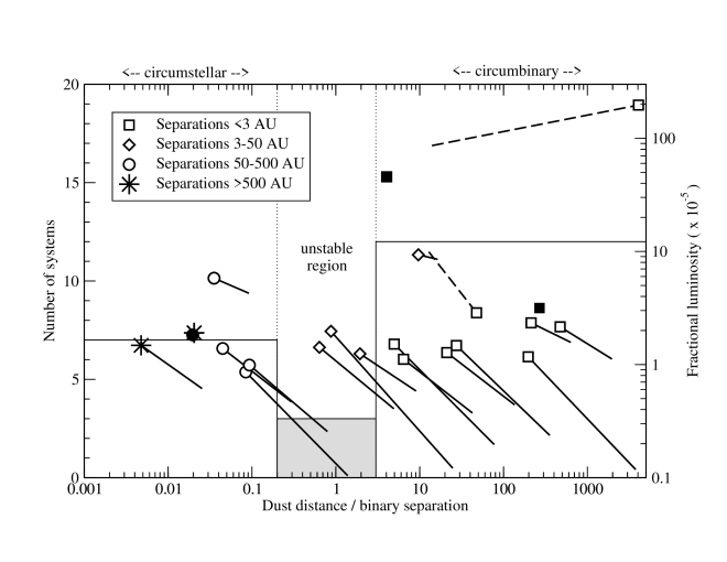
Figure 5: Histogram of dust distance in units of binary separation (left axis) and fractional luminosity as function of dust distance in units of binary separation (right axis). Left axis: The dashed vertical lines show the approximate boundaries of the unstable zone (histogram bar shaded grey). Dust in two systems is found to reside within this dynamically unstable region (Table 4). Right axis: There is no strong trend between fractional luminosity and dust location. Binary systems with small, medium, large, and very large physical separations are indicated. Not surprisingly, circumbinary disks are generally found in small separation systems and circumstellar disks are found in large separation systems. Dust in unstable regions is found only in separation systems, as expected (Section 6.6). Fractional luminosities for the maximum temperature cases are indicated by the symbols. “Tails” on the symbols indicate the locus of solutions, from maximum temperature solutions (symbols) to 50 K (minimum reasonable) solutions at the other ends of the tails. (There are two exceptions, where we instead use the cool solutions as our best solutions. The range of solutions for these two systems extends to the left in this plot, as described in Section 5.3. We show those ranges as dashed lines because we have no good upper bounds for these systems.) The range of solutions generally is not large enough to change our dynamical classifications substantially. The four symbols without tails (two filled squares, one filled circle, and one star) indicate systems with excesses at both 24 and 70 µm (Table 4). Because the color temperatures of the excesses are known for these four systems (through the detection of the excesses at multiple wavelengths), the locations of these symbols on this plot cannot change significantly, so no tails are given.

We derive fractional luminosities for each system; because we fit maximum temperatures to the infrared excesses, the derived fractional luminosities are also maximum values. We explore in Section 8.1 the impact of the “minimum” temperature alternate assumption on fractional luminosity. We list the derived fractional luminosities for all 22 systems with formal excesses in Table 4; these fractional luminosities are plotted in Figure 5. Systems with excesses at 24 µm generally have large fractional luminosities because the dust temperatures are warm. This can be seen in Table 4, where the largest fractional luminosity is for HD 83808, the system with the highest excess temperature. We discuss the details of that system in the following section.

Our fractional luminosities are mostly in the range $10^{-5}$ to $10^{-4}$ (Table 4 and Figure 5). This range is consistent with values found by other surveys of debris disks around “old” stars (as described in Section 9). We show in Figure 5 fractional luminosity as a function of dust distance in units of binary separation; there is no obvious trend. There is an apparent limit near $10^{-5}$, which is approximately the MIPS detection threshold (see also Bryden et al., 2006).

Our observations at 24 and 70 µm place no constraints on colder ($\sim$30 K) disk components. Our 13 submillimeter upper limits preclude the existence of very massive cold disks but place no useful constraints on modest (fractional luminosity $\sim$10^-5) cold disks. Although we refer to the fractional luminosity values we derive as maximum values, it is worth noting that a cold, massive disk component could exist for almost all systems in our sample. This putative cold disk could imply a larger fractional luminosity than the “maximum” values that we report here.

5.3 Systems of interest

We show six systems of particular interest in Figure 1, and discuss them here. These systems present the most interesting and illustrative cases for SED fitting. An additional 13 systems of note are discussed in Appendix B.

HD 13161, HD 51199, and HD 16628. These three systems all have formal excesses at both 24 and 70 µm (Figure 1). We therefore have a very good measurement of the color temperature of the excess. HD 13161 was identified as Vega-like — meaning likely possessing a debris disk — by Sadakane & Nishida (1986) as well as a number of later workers, based on IRAS fluxes. HD 51199 has a relatively strong excess at 24 µm and a relatively weak excess at 70 µm, implying a somewhat high dust temperature of 188 K. The 70 µm flux for HD 16628 is more than five times brighter than the expected photospheric flux.

HD 83808. HD 83808 also has formal excesses at both bands (Figure 1). This two-band fit gives an excess temperature of 815 K; comparable excesses at 24 and 70 µm (23% and 30%, respectively) indicate that the excess color is only slightly redder than the star(s), implying a relatively high excess temperature.

Because this temperature is quite high compared to a typical dust disk result in this program, we use IRAS measurements for a consistency check. The color-corrected IRAS fluxes are 3500, 800, and 130 mJy at 12, 25, and 60 µm, respectively; this implies 24 and 70 µm fluxes of 870 and 96 mJy, respectively (after scaling by $\lambda^{2}$). (We note that the IRAS 60 µm measurement formally has quality flag 1, meaning an upper limit, but the measurement is consistent with our higher S/N observation.) Our 24 and 70 µm measurements of 822 and 94 mJy, respectively, match the IRAS data quite well. We can extrapolate our 24 µm measurement to 12 µm (again scaling by $\lambda^{2}$), and get 3500 mJy, again matching the IRAS measurement. We conclude that the IRAS data are consistent with our measurements.

Now we look again at the IRAS data for confirmation of our excess temperature. The predicted photospheric fluxes (combining IRAS and MIPS data) at $\lambda$ = [12,24,25,60,70] µm are [2600, 670, 600, 103, 72] mJy (after color correction). The observed fluxes are [3500, 822, 800, $<$130, 94] mJy (after color correction). This implies a 12 µm excess of 900 mJy. An 815 K dust population would imply an excess at 12 µm of around 400 mJy, for a total (color-corrected) 12 µm flux of $\sim$3000 mJy. Since the error on the IRAS 12 µm data is 6%, the measured IRAS 12 µm flux of 3500 mJy is consistent at a two sigma level with emission from an 815 K disk, and may even imply a hotter temperature for the excess. We therefore feel confident in the determination of an 815 K excess for this system, based on detections at both MIPS bands and an IRAS 12 µm excess. This temperature is one of the hottest debris disk temperatures known.

We note that the primary of HD 83808 has moved off the main sequence (see Section 8.5 and Hummel et al. (2001)). This should not have any significant effect on our SED fitting or analysis of excess emission from this system, but adds to the complexity of this system. For example, it is possible that this giant star could be ejecting dust, and that the hot excess we observe may represent a dust shell rather than a debris disk. We also note (from Simbad) the presence of a radio source and an X-ray source within about 15″ of HD 83808; if these sources are related to the HD 83808 system then further complexities may be implied.

HD 118216. This system shows a 47% excess at 24 µm (Figure 1). We did not observe this system at 70 µm because its predicted 70 µm flux suggested that, in the absence of any excess emission, we would not have detected the photosphere at greater than 3$\sigma$ precision. The single bandpass (24 µm) detection unfortunately does not allow us to constrain the system’s SED, shown in Figure 1, or the color temperature of the excess, and we must turn elsewhere to improve our understanding of this excess emission.

The IRAS 12 µm flux measurement, after color correction, is greater than the predicted 12 µm photospheric flux by about 1.7 sigma (measurement error, not including calibration error). One approach would be to assume that this 12 µm measurement is indicative of excess flux; that logical path implies a maximum excess temperature around 850 K. However, we are reluctant to place too much emphasis on a 1.7 sigma “excess” and look elsewhere for additional constraints.

In Section 8.1 we argue that the minimum reasonable dust temperature is 50 K for all systems. Hence, we calculate the fractional luminosity for 50 K dust in this system by forcing the emission from the dust to pass through the measured 24 µm flux value. In doing so, we find that the hot (here, 850 K) solution has a lower fractional luminosity than the cold (here, 50 K) solution, in contrast to the pattern typically seen for debris disks detected in this program (Figure 5). Because of our lack of good constraints for this system, we present this minimum (and hence conservative) solution in Table 4 and Figure 5 as our “best-fit” solution. As usual, Figure 5 shows the best-fit solution (here, 50 K) as a symbol, with a tail extending to the extreme other solution (here, 850 K, from the above analysis). A dashed line is used for this tail to indicate that more assumptions than usual were made for this system. Note that, in comparison for most other systems with excesses in our sample, for HD 118216 we derive a lower limit on the temperature.

As a consistency check, we use the IRAS 60 µm upper limit of 171 mJy (Moshir et al., 1989) to derive a temperature for the excess. We subtract the predicted photospheric flux at 60 µm and ascribe the difference from the upper limit (133 mJy) as all due to potential excess. Using this 60 µm “excess” and our 24 µm (MIPS) measurement we find a color temperature of 134 K. To pick a representative temperature, we show this 134 K fit in Figure 1 (but use the bounds 50–850 K elsewhere in this paper). This temperature falls within the bounds presented above of 50–850 K, and so is consistent with our bounds given above, but it is clear that further data on this target would help eliminate the need for some of the above assumptions and better constrain the dust temperature.

HD 16920. For this system we formally detect an excess at 24 µm and formally do not detect an excess at 70 µm, where the excess ratio of 1.22 does not meet our excess criterion and where $\chi_{70}$ of 1.22 may indicate that there is no significant excess for this system at 70 µm (Figure 1). The IRAS data are consistent with our observations.

Because we have data at both MIPS wavelengths, here we can follow the process described above for the case of a clear excess at one wavelength and no excess at the other wavelength. We fit a blackbody to the measured 24 µm data (where the excess is found) and the predicted 70 µm photospheric flux plus three times the error at 70 µm (see Table 3). For an excess at 24 µm and no excess at 70 µm, this technique gives a minimum temperature for the excess (through an upper limit on the 70 µm flux). This minimum excess temperature is 260 K. With no evidence of excess in the IRAS 12 µm data, we must additionally make a “maximum temperature” assumption. We choose 500 K, which is similar to the temperature derived for the dust in HD 69830 (Beichman et al., 2005b) and is warmer than almost all derived debris disk temperatures from this and other programs. We solve for the fractional luminosities for these bracketing temperatures, again forcing the derived excess emission profile to pass through the observed 24 µm point. We use the 260 K solution as our best fit, shown in Table 4, Figure 1, and Figure 5.

It is unusual in our MIPS surveys for debris disks to show formal excess at 24 µm and not at 70 µm (for systems strongly detected at both wavelengths). The best example of a system with that unusual excess pattern is HD 69830, which Beichman et al. (2005b) interpret as hot dust created in a very recent asteroidal or cometary collision. We argue below that at least two binary systems with excesses also show evidence of recent dust-producing collisions. Note that HD 69830 was recently found to have three planets orbiting that star (Lovis et al., 2006), perhaps further linking 24 µm only excesses with planetary system formation.

6 Dynamics: Where is the dust?

6.1 Stability in binary systems

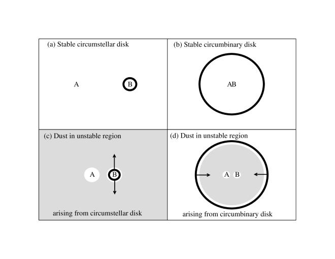
Figure 6: Schematic diagrams of the four cases for dust in binary systems. All features of each panel are to scale. In all four panels, “A” and “B” refer to the two stars and the thick, dark bands represent the location of the planetesimal population, which is in a stable location in all four panels. In all cases, dust is assumed to be produced in the planetesimal belts. Cases (a) and (b) correspond to observations of dust in stable circumstellar and circumbinary locations, respectively, with the implication that the dust is observed near its creation location in the planetesimal belt. For panels (c) and (d), the grey shaded area shows the unstable region as defined in the text. Cases (c) and (d) show two possible mechanisms to transfer dust (radial arrows, ignoring orbital motion) from a stable planetesimal population to the unstable region where it is detected. Outward motion, shown in panel (c), is caused by radiation pressure, while inward motion, shown in panel (d), is caused by PR drag. Case (d) but not Case (c) is consistent with excess emission at 70 µm but no excess emission at 24 µm. All three systems with unstable dust have excesses only at 70 µm, implying that Case (d) is likely to be the dominant mode of radial transport.

Holman & Wiegert (1999) carried out a study of the stability zones in binary systems by placing test particles in binary systems with a range of mass ratios and eccentricities; in all cases the test particles have zero eccentricity. (A similar stability study was carried out by Verrier & Evans (2006) for the planet-bearing binary system $\gamma$ Cephei.) Holman & Wiegert derive a “critical semimajor axis,” $a_{c}$, which is the maximum (for circumstellar material) or minimum (for circumbinary material) semi-major axis where the test particle is stable over $10^{4}$ binary periods, though resonances may reduce stability even in regions safely beyond $a_{c}$. For circumstellar material, the critical radius within which material is stable is typically 0.1–0.2 in units of the binary separation; for circumbinary material, the critical radius outside of which material is stable is typically 3–4 in the same units (Figure 6). The locations of these stability boundaries change for various binary eccentricities and mass ratios — information that is known for some of the binary systems with excesses (see Table 4) — but these changes are relatively small for most of the binary systems we consider. Whitmire et al. (1998), in a similar study to Holman & Wiegert (1999), found an unstable zone that is somewhat broader (that is, a greater range of orbital distances that are unstable), as did Moriwaki & Nakagawa (2004) and Fatuzzo et al. (2006). To be conservative in our identifying dust in unstable disks (that is, to identify a lower limit on the number of unstable disks), we adopt the Holman & Wiegert (1999) criteria, and note that using the broader instability zones would increase the number of systems with dust in unstable locations. As a caveat, we note that the Holman & Wiegert stability criteria only apply to test particles that experience no non-gravitational forces, and therefore do not explicitly apply to dust. However, their stability arguments do apply to the asteroidal bodies that collide to produce dust (Section 6.3).

6.2 Debris disk geometries in our sample

We apply the Holman & Wiegert stability criteria to the debris disks in the 22 systems with excesses (Table 4). Dust may reside in stable circumstellar or stable circumbinary regions, or in unstable regions as defined by Holman & Wiegert; these different cases are shown schematically in Figure 6. Twelve of the 22 systems with excess have dust distances that are much larger than the system’s binary separation, implying a circumbinary debris disk. Not surprisingly, all but one of these circumbinary debris disks is in a small separation system (and the separation for the one exception is still only 5.3 AU). Seven of the 22 systems with excesses have dust distances that are much less than the system’s binary separation, implying circumstellar debris disks. (We have assumed that the debris disk surrounds the primary star but we have no way to verify this for systems that are not resolved.) All of these systems have binary separations greater than 75 AU. Three systems with excess do not obviously have either circumbinary or circumstellar debris disks, but rather have dust distances that imply unstable locations, that is, dust distances that are similar to the binary separations. These three systems (HD 46273, HD 80671, HD 127726) are discussed further in Section 6.4. The dynamical classification of each system (circumbinary, circumstellar, or unstable) is listed in Table 4, and a histogram of systems in these three dynamical states is shown in Figure 5.

For the four systems with excesses detected at both 24 and 70 µm, the dust temperature is uniquely fit to the two-band excess; these systems are plotted in Figure 5 with filled symbols. Three of these four systems have circumstellar dust, and one has circumbinary dust. For systems with excesses at only one band, we show in Figure 5 the maximum temperature solution and a range of solutions for each system. The range of solutions lies between the maximum temperature solution (symbols) we derive from the data and the minimum temperature (50 K) solution (Section 8.1) and its corresponding dust distances and fractional luminosities (end of the “tail” on the data point). (Two systems have the reverse situation, in which the best solution is a minimum temperature solution and the range of solutions allows warmer temperatures and consequently smaller dust distances; these two cases are indicated with dashed tails in Figure 5.) Because for most systems a range of solutions is allowed, and because the boundaries between stable and unstable regions may have some flexibility, we note that some reclassification of dynamical states may be possible. However, the overall distributions shown in Figure 5 are unlikely to change substantially. For the four systems with excesses detected at both 24 and 70 µm, the dust temperature is uniquely fit to the two-band excess, and consequently no range of solutions is shown in Figure 5; these systems are plotted with filled symbols.

6.3 Dust and precursor asteroid belts

We explain our detections of excess emission conceptually as due to a belt of asteroids that collide, producing dust. This dust may be observed at its generation location. For both the circumbinary and circumstellar cases, the simplest explanation is the presence of a planetesimal belt near the distance that we derive. We ignore the possibility of dust produced from parent bodies that reside in the unstable region, as the lifetimes of those parent bodies in the unstable regions are prohibitively short (Holman & Wiegert, 1999). However, dust can move radially due to radiation pressure or Poynting-Robertson effect, and therefore can have a very different emission temperature than it had in its generation location (its asteroid belt). (In fact, the Holman & Wiegert (1999) calculations for stability do not apply for dust, but do apply to the dust parent bodies.) This may be the explanation for dust in unstable regions in the HD 46273, HD 80671, and HD 127726 systems, as described in the following section.

6.4 Dust in unstable regions

Dust in an unstable location could be migrating inward (under PR drag) from a larger radius (and potentially circumbinary disk), or could be migrating outward (via radiation pressure) from a smaller radius and a circumstellar disk (Figure 6). The parameter $\beta$ is often used to examine radial migration of dust grains. It expresses the ratio of radiation to gravity forces on an individual dust grain: $\beta=(3L_{\star}/16\pi GM_{\star}c)(Q_{pr}/\rho s)$, where $L_{\star}$ and $M_{\star}$ are the stellar luminosity and mass; $c$ is the speed of light; $Q_{pr}$ is the radiation pressure coefficient (we use $Q_{pr}=0.35$, after Moro-Martín et al., 2005); and $\rho$ and $s$ are the density and radius of the spherical grain, with all values in cgs units. Grains that have $\beta<0.5$ generally spiral inward under Poynting-Robertson (PR) drag (e.g., Moro-Martín et al., 2005). $\beta$ values greater than 0.5 correspond to dust particles that are blown out of the system by radiation pressure. A critical size can be derived, where spherical, solid particles larger than that size spiral inward under PR drag. For A5 stars, the critical size is $\sim$5 µm; for F5 stars, the critical size is $\sim$2 µm. Of course, the picture is somewhat more complicated when there are two stars in the system since both radiation and gravity increase; furthermore, a particle may not see a simple radial radiation pattern as from a single central source. (We revisit these complications below.) Particles also need not be solid spheres in reality.

We have assumed black body grains, where the particles are larger than the wavelengths of interest. Thus, the infrared excesses that we observe are generally emitted by dust grains larger than the critical size of around 5 µm or so. Such large grains are plausible in debris systems, although we consider the case of small grains in Section 8.2. These grains should therefore be spiraling inward under PR drag, suggesting exterior production zones.

As a further argument, our temperature (and distance) derivations solve for the maximum temperature allowed by the data; in other words, there can be no significant population of dust interior to the distances that we derive. Yet, if the dust were migrating outward from an interior source, there would necessarily be a population of dust that would be warmer and at smaller distances than the observed dust location. Dust closer to the star(s) and warmer would have been detectable by us, yet R24 for these two systems is within 3% of unity. For these systems, the dust therefore cannot originate in an interior source region, as we would have detected it at 24 µm.

These arguments are consistent with our results that the most common configuration of dust in binary systems is in stable circumbinary regions. In 12 cases (out of 22 total), dust is created and observed in circumbinary locations. In an additional two systems, we suggest, dust is created in circumbinary locations and migrates inward under PR drag to an unstable location where we observe it (Figure 6).

Wyatt (2005) and others have suggested that in debris disks with large enough optical depth to be observable, PR drag should never dominate; instead, removal of grains that are big enough to be in the PR (as opposed to radiation pressure) regime will instead be dominated by collisional processes. (Note that in the Solar System, whose fractional luminosity is perhaps a factor of $\sim$100 less than those for typical Spitzer-discovered debris disks, PR drag can be a dominant source of grain removal (e.g., Moro-Martín & Malhotra, 2002).) Indeed, Chen et al. (2006) provide observational evidence that IRAS discovered debris disks are dominated by collisions and not PR drag. In the planetesimal belt where the dust we observe is originally produced, it may be true that the space density of grains is high enough that collisions dominate. We calculate that $\eta_{0}$, defined by Wyatt (2005) as the ratio of PR migration timescale to collisional disruption timescale, is generally close to but slightly larger than unity for the disks detected in this program ($\eta_{0}\gg 1$ means collisions dominate; $\eta_{0}\ll 1$ means PR dominates). This implies that most grains of the size of interest collide with other grains before they migrate inward a significant distance, but also implies that some grains may migrate inward under PR drag without experiencing any collisions. Furthermore, the belt where collisions are taking place must have an inner edge that is defined by the binary’s dynamical interactions. Grains that leak inward across this boundary may suddenly be in a region that is devoid of solid material, since no planetesimals would be in stable orbits there. In this “empty” region, few collisions would take place and little dust would exist, other than dust migrating inward under PR drag. PR effects would dominate since the surface density of grains would be relatively small, implying that collisions cannot be a significant loss mechanism. This may be the dust that we observe in radiative equilibrium with the binary stars.

6.5 Detailed analysis of systems with dust in unstable locations

HD 46273. HD 46273 is a member of a quintuple system. HD 46273 is the AB pair, with a separation of 0$\farcs$5 or 25.9 AU (Table 1). The AB-CD separation is 13$\farcs$4 (Worley & Douglass, 1997), or about 700 AU (27 times the AB separation). We detect the CD members of the HD 46273 system in our MIPS images, clearly resolved and outside our photometric aperture at 24 µm and very marginally resolved (and very faint) at 70 µm. At most, the CD stars account for 15% of the measured flux at 70 µm, indicating that the excess at this wavelength cannot be due simply to including flux from the CD stars in our photometry. Finally, component A is a spectroscopic binary, with members Aa and Ab.

Our best fit maximum temperature solution places the dust at 16 AU. We recall that the stable regions in a binary system are roughly bounded by orbital distances three times less/greater than the binary separation. Stable orbits are therefore found in the range 80–230 AU from component A (bounded on the inside by the AB pair and on the outside by the AB-CD interaction). If the Aa/Ab separation is less than 2.6 AU, then another stable region would exist from three times the Aa/Ab separation out to 8 AU. None of these zones clearly imply dust temperatures of $\sim$100 K. However, in light of the extremely complicated dynamics and radiation and gravity fields in this system, it is clear that our first-order calculations of dust distance and long-term stability may not be sufficient.

HD 80671. HD 80671 is in a triple system, where the AB pair has a separation of 0$\farcs$12, or 3.35 AU (Table 1). The AB-C separation is 18$\farcs$1 (Worley & Douglass, 1997) or 500 AU, around 150 times greater than the AB separation. We calculate a dust distance of 2.9 AU. The existence of component C places no significant constrains on the location of the dust, and in this system, it is (more) likely that the C component plays little or no role in the gravity and radiation effects of the AB system, where the dust is. The interpretation may therefore be more straightforward and more similar to the first-order model we have presented above.

HD 127726. HD 127726 is also a triple system, with an AB separation of 14.3 AU (0$\farcs$2). The AB-C separation is 2$\farcs$0, or around 143 AU (Worley & Douglass, 1997). For this system, the critical outer radius for the AB pair is nearly equal to the critical inner radius for the AB-C system, implying that there are no stable regions in this system between around 4.5–430 AU. This stability argument leaves in question where a stable asteroidal population could reside, from which the observed dust can migrate. Further study may help reveal the nature of this interesting system.

We note that all three systems with dust in unstable locations are multiple (higher than binary) systems. As argued above, this multiplicity may complicate the radiation field sufficiently that the dust has a temperature that masks its true location in a stable location. Alternately, more complicated gravitational interactions may promote asteroid collisions, producing dust that is short-lived (Section 7.2). It is unlikely that a location that is unstable in a binary system would be stable in a multiple system, barring unusual resonant configurations. Finally, for these systems (and others in our sample) there could be multiple reservoirs of dust, each having different temperatures and located in a stable location in the system, that together masquerade as a dust population with the single temperature that we derive from a 1 or 2 band excess.

6.6 Dust at 10–30 AU: Confirmation of expectations

Our observations at 24 and 70 µm are generally sensitive to dust temperatures around 50–150 K, which are found at distances of 10–30 AU around A and F stars. Since dust is more likely to be found in stable regions of binary systems than in unstable regions (from dynamical arguments), we are less likely to detect excess emission from binary systems with separations of 10–30 AU than from those with either smaller or larger separations. Figure 4 shows that, indeed, we observe fewer excesses for intermediate separation systems, as we expect. We conclude that the stability arguments of Holman & Wiegert (1999) must apply generally to dust in binary systems. We note that this distribution of excess as a function of binary separation is consistent with the result of Jensen et al. (1996).

The complement of this argument is that we are more likely to detect dust in unstable zones for intermediate separation systems than for either small or large separation systems, for the same reason: dust at 50–150 K that is unstable is more likely to be found in intermediate systems (by the Holman & Wiegert arguments) than in either small or large separation systems. We find this result as well (Figure 5): all three systems with dust in the unstable region are binaries with intermediate separations, as expected.

7 Planetary system formation in binary systems

7.1 Nature versus nurture

A primary conclusion from this study is that debris disks exist in binary systems. Planetesimal formation clearly is not inhibited to any great degree by the presence of a second star in the system. Whether planetary system formation advances beyond the planetesimal stage cannot be addressed by this work. However, we can comment on the kinds of dust-producing interactions taking place among planetesimals in these systems.

The anti-correlation between age and debris disks has been well explored (e.g., Rieke et al., 2005; Siegler et al., 2006; Gorlova et al., 2006; Su et al., 2006), and the slopes of such functional relationships typically asymptote to zero for ages 500 million years and older. For systems older than this, stochastic or random processes may dominate the production of dust (e.g., Rieke et al., 2005; Su et al., 2005), and not the gradual diminishing of an initial disk reservoir. However, a continuous collisional cascade over the lifetime of the system remains a possible explanation.

The excess rate we find for binary systems is marginally higher than that for individual (single) stars (Section 9.1). One possibility is that multiple stellar systems may begin with circumstellar/circumbinary disks that are more massive than those surrounding single stars – the nature argument. Hence, multiple stellar systems are more likely — from birth — than individual stars to possess planetesimal disks and planetary systems, and therefore excess emission that we can detect.

Alternately, multiple stellar systems may begin with circumstellar/circumbinary disks that are similar to or diminished relative to disks around individual stars. The multiple stars may then interact in ways that could cause planetesimal growth (and subsequent dust production): the two (or more) stars present in the system can stir up the circumbinary (or circumstellar) disk, causing orbits to cross and generally creating an environment in which accumulation of solid material in a protoplanetary disk is favored. This is the nurture argument, that multiple systems create environments where planetary systems may be more likely to form (Marzari & Scholl, 2000; Boss, 2006).

We note that this nurture model may have a significant backlash. Enhanced dynamical stirring could equally be the downfall of planet formation if protoplanetary disk material is excited sufficiently that collisions are erosive rather than accumulative. Thébault et al. (2006) find that the boundary between these two regimes depends on the size of the interacting bodies, among other parameters, implying that within a single system collisions could potentially be erosive for asteroid-sized bodies ($\sim$10 km) but accumulative for larger bodies.

Determining which of nature and nurture is more important in planetesimal formation in multiple systems will require detailed studies of the youngest multiple systems (e.g., the results presented in Jensen et al. (1996) and McCabe et al. (2006)). Further disk studies of an ensemble of young binary (or higher) systems will allow us to understand the initial conditions that lead to the properties of the sample presented here.

7.2 Residence times and collisions in binary systems

Particles in the unstable zone have their orbits disrupted in $\lesssim$$10^{4}$ orbits of the binary system (Holman & Wiegert, 1999). The orbital periods for HD 46273, HD 80671, and HD 127726 are all less than 100 years, so the dust should be removed in less than 1 million years in all cases. The PR crossing time $\tau_{PR}$ is given approximately by $400(\Delta r)^{2}/M_{\star}\beta$, where $\tau_{PR}$ is in years; $\Delta r$ is the radial distance to be crossed, in AU; $M_{\star}$ is in Solar masses; and $\beta$ is as defined above (Wyatt, 2005). The unstable zone extends approximately from 0.3 to 3 times the binary separation, so we set $\Delta r$ equal to 2.7 times the binary separation. The PR crossing times, which are the maximum residence times of dust in the unstable zone, are therefore also around 1 million years for these systems. These facts together imply that the dust residing in these unstable regions is very short-lived and that we are witnessing either the migrating tail of a continuous cascade, or the result of a very recent collisional event (see, e.g., Lisse et al., 2007). With a few assumptions, we may be able to suggest which of these is more likely.

For these three infrared excess systems, the residence time of dust against loss mechanisms is around $10^{6}$ years and the typical fractional luminosity is around $10^{-5}$. For the purposes of this exercise, we assume 10 µm dust grains located 10 AU from a parent star. In this case, approximately $10^{30}$ grains are required (at low optical depth) to absorb and re-radiate the appropriate amount of emission from the parent star. For a density of 1 g/cm³, this population of grains has a mass of $\sim$4$\times 10^{21}$ g. For a residence time of $10^{6}$ years, this implies a grain production rate on the order of $10^{8}$ g/s, similar to that measured for comet Hale-Bopp (Lisse et al., 1997). This is a small enough production rate that none of continuous collisional cascade; stochastic collisions; or individual sources (e.g., comets) can be ruled out. The ages for the two systems with dust in unstable locations are 1–2 billion years. Over 1 billion years, the total mass of 10 µm dust grains produced under a continuous collisional cascade would be around $3\times 10^{24}$ g or $5\times 10^{-4}$ $M_{\oplus}$, which implies the efficient disintegration of $\sim$1000 hundred-km asteroids. If the 10 µm grains are the tail of a size distribution that follows a power law that goes as size^-3.5 (e.g., Dohnanyi, 1969), the total mass may be 10–100 times greater; a shallower slope (e.g., Reach et al., 2003) gives an even larger enhancement. In our Solar System, there are fewer than 400 asteroids larger than 100 km. Over the age of the Solar System, the number of 100 km asteroids in the asteroid belt may have decreased by only a factor of 5–10 (e.g., Davis et al., 2002). Our Solar System’s asteroid belt could therefore not be the source of a continuous dust production of the magnitude that is presently observed for these two systems. The implication may be that the present dust production rate cannot have been continuous over the lifetime of the system. Although other interpretations are possible, this rough calculation implies that the dust that we observe in these systems was likely produced in a recent event, and that stochastic (occasional) collisions may dominate the dust production in these systems on billion-year timescales.

8 Alternate interpretations and uncertainties

8.1 Uncertainties in dust temperatures

Several alternate interpretations can explain the observations and dynamical stability constraints. Recall that the dust temperatures presented in Table 4 and elsewhere are the maximum temperatures allowed by the multi-wavelength observations (with the two exceptions described above and noted in Table 4; these exceptions are addressed below). In general, this is the most rigorous and most useful statement that can be made, but cooler temperatures might equally well fit the data and imply greater orbital distances, with implications for the implied stability.

To explore the consequences of abandoning our maximum temperature requirement, we recalculated dust location and fractional luminosity for systems with only 70 µm excesses assuming that all the dust has a “minimum reasonable temperature” of 50 K, a value that is consistent with the smallest excess temperatures found by Su et al. (2006). (Note that this is not truly the absolute minimum possible, since an undetectable population of very cold dust cannot be ruled out for any system.) In all cases 50 K is consistent with a physical model that can match the observations, and corresponds roughly to a 24 µm excess that is $\sim$1% of the photospheric emission. Generally, the dust location increases somewhat in radius and the fractional luminosity decreases by up to a factor of 10. These alternate (minimum) solutions are shown in Figure 5 as the ends of the “tails” extending from the data points. The locus of acceptable solutions for each system lies along this tail, with the maximum temperature solution at one end (indicated by the symbol) and the minimum temperature solution at the other end. Alternate solutions, with different temperatures, could potentially move systems into or out of the unstable zone, and in all cases include a move to lower fractional luminosities.

For the two systems where the best temperature solutions are lower limits (HD 118216 and HD 16920), the “tails” indicate that warmer temperatures (that is, smaller dust distances) are possible solutions. In each case, assumptions were needed to calculate the range of acceptable temperatures (Section 5.3); because of these extra assumptions, these tails are shown as dashed lines.

8.2 Non-black body dust grains

We have assumed black body dust grains for all analysis and discussion above, but non-black body dust grains (generally those with small sizes) offer a possible alternative interpretation. Non-black body grain thermal equilibrium temperatures are hotter than those of black body-like grains at the same distance from the star (see, e.g., Su et al., 2005, and Figure 9 therein). Therefore, in matching a derived temperature, non-black body grains would imply a greater distance from the star(s) than the black body grain solutions discussed above. Under Mie theory, the dust distance (in centimeters) is given by $(R_{\star}/2)(T_{\star}/T_{g})^{2.5}$ where $R_{\star}$ is the stellar radius (in centimeters), and where the grain temperatures are those derived in Section 5.2.2. Calculating dust distances under this small-grain assumption moves all systems rightward in Figure 5, and moves some systems from the circumstellar region to the unstable region, and some from the unstable region to the circumbinary region. However, the total number of systems in the unstable region is unchanged: even under this small-grain assumption, there still exist populations of grains in unstable regions.

Smaller grains might also have $\beta>0.5$. This means that grains might be spiraling outward under radiation pressure. It would still be difficult to explain any dust that remains in the unstable zone, since there is no evidence for hotter interior reservoirs of dust, as explained above. A more difficult case would arise if the grain properties vary significantly from system to system. We leave a more complete exploration of these effects for future work as the number of free parameters is large enough that useful constraints may not be easily obtained.

8.3 Uncertainties in dust location

A final uncertainty on our calculations of grain temperatures is related to the geometry of the systems. We have implicitly assumed that all radiation fields are purely radial, and that all flux comes from a single source, either as a combined close binary or a single star whose companion is far away. For the two systems where the implied dust distances are comparable to the binary separations — that is, for systems where the dust appears to be in the unstable region — neither assumption is likely to be true. More sophisticated modeling that considers the specific geometry of a given system would be appropriate in those cases.

There are a number of other potential geometries. We have assumed in all cases that any circumstellar dust must be located around the primary, whose spectral type is known, but of course dust in a binary system could equally be around either the primary or the secondary. A more complicated geometry would allow for circumsecondary dust, but a luminosity ratio for which the primary significantly heats the dust as well; such a construction could even masquerade as a dust population located in the unstable zone.

Following from the previous discussion, there is potentially substantial uncertainty in the dust location for any given system. Even for systems with excesses at both wavelengths, the possibility of non-black body grains could allow for a substantial change in dust distance. There is little to be done to explore the consequences of these uncertainties as we have no more than two excess measurements for any system. Further observations at different wavelengths, and especially including low resolution spectra that would allow us to map the SED at much higher resolution than broadband photometry permits, are necessary to break some of these degeneracies and remove uncertainties (see, e.g., Su et al., 2006, and Figure 13 therein). Spatially resolved images at multiple wavelengths would also help break these degeneracies.

Finally, we model all dust populations as single populations at a single location. For the four systems with excesses at both bands, there exists the possibility that dust could instead reside in two separate reservoirs: a hot dust population near one of the stars and a cold(er) circumbinary dust population. The small number of data points does not warrant further calculations of this possibility, but we mention it against the possibility of future data that may help constrain the location of the dust in that system. For the three systems with dust apparently in unstable locations, having multiple dust populations in different (stable) locations could masquerade as a single population in an unstable location.

8.4 Uncertainties in binary separations

In some cases, the separations listed in Table 1 (and Table 4) are the projected separations, not the actual orbital distance. This is because some of these binary systems have not been monitored long enough or well enough to determine true orbits for the components. To calculate whether the dust we observe is in an unstable region, we use the separations in Table 1, which lists the best information we have (actual or projected separations). Some of our determinations of dust in unstable regions, therefore, could in theory change categorizations if the separation information changed substantially. We suspect that this possibility would contribute only a minor effect overall as projected separations are not likely to differ from orbital separations by more than a factor of $\sim$2 in most cases. We also note that higher multiplicity (beyond binarity) may have an effect in the stability of planetesimal belts and the production of dust (Section 6.5).

8.5 Possible youth effects

Ages are known for most, but not all, of these 69 binary systems (Table 1). As it is now well established that larger excesses generally are found around younger stars (e.g., Rieke et al., 2005; Su et al., 2006; Gorlova et al., 2006; Siegler et al., 2006), we look for possible effects of youth in our results.

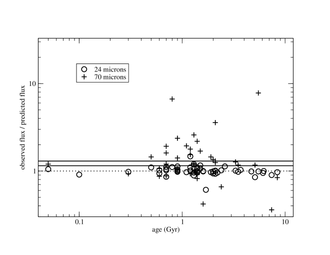
Figure 7: Ratio of observed to predicted fluxes for all systems as a function of system age, for systems with known ages. Circles show data for 24 µm observations and crosses show results for 70 µm observations. In all cases the errors in R24 and R70 are smaller than the symbols. The solid horizontal lines show our criteria for identification of excess at R24 = 1.15 (lower line) and R70 = 1.30 (upper line), and the dotted line shows R = 1.00, for guidance. No obvious trend of excess (observed/predicted) with age is apparent, though we note that several of the systems with large excesses have no published ages and hence are not shown here (see text for discussion); we cannot rule out the possibility that these systems with large excesses are young.

R24 and R70 as a function of age are shown in Figure 7 for the 55 systems with known ages. One might expect that the younger systems would be more likely to have detectable excesses (e.g., Habing et al., 2001; Dominik & Decin, 2003; Rieke et al., 2005; Su et al., 2006; Gorlova et al., 2006; Siegler et al., 2006). However, since most systems with known ages in this program are older than 1 billion years, and all are older than around 600 million years (with three exceptions, as indicated in Table 1), these systems are all mature, so any age dependence might be expected to be minor. Indeed, we find no obvious trend of excess with system age (Figure 7), though we note that several of the systems with large excesses have no published ages and hence are not shown here (see text for discussion); we cannot rule out the possibility that these systems with large excesses are young.

There are 14 systems for which no published or calculated ages are available. However, we can classify ten of these systems as “old” or “young,” as follows; since we are looking for possible effects of youth, this rough classification suffices.

HD 83808, HD 13161 (a large excess system), HD 17094, and HD 213235 are all more luminous than dwarf spectral classes, according to the Gray & Corbally technique (see Table 1 and Appendix A). These systems (or at least the primary stars) are therefore likely at the old end of their main sequence lifetimes (and have started to evolve off the main sequence). HD 137909 is part of an extensive study by Hubrig et al. (2005), who put it on the HR diagram and find it to be well above the ZAMS, implying that this system is old. These systems are labeled “old” in Table 1, indicating that excesses around HD 83808, HD 13161, and HD 17094 cannot be due to youth effects.

HD 127726 (70 µm excess) and HD 50635 (no excesses) were both detected by ROSAT (Hunsch et al., 1998). Both stars have spectral types F0V, which may be too early for chromospheric activity, so a likely scenario is the presence of an active late-type dwarf companion. This argues for youth for these systems, but is not a strong constraint, since the main sequence lifetimes of late-type dwarfs are much longer than those for F0 main sequence stars. We label both HD 127726 and HD 50635 “young” in Table 1. Indeed, Barry (1988) estimate a chromospheric age of 300 Myr for HD 50635 based on Ca II H and K measurements of the secondary. However, Strömgren photometry (Mermilliod et al., 1997) of the HD 50635 primary alone is available (due to the system’s relatively wide separation), and suggests an age of 990 Myr (using the Moon & Dworetsky (1985) grid of stellar parameters), indicating that our designation of “young” for this system has substantial uncertainty.

HD 61497, like HD 50635, is widely enough separated that the primary alone can be identified in Strömgren photometry (Mermilliod et al., 1997). Again using the Moon & Dworetsky (1985) grid of stellar parameters, we estimate an age of 520 Myr for this system, and we therefore label it “young” (following our definitions of “young” and “old” in Section 9.1).

Finally, we use the $\log g$ values presented in Table 1 to conclude that HD 72462 is old and that HD 6767 is young, based on their low and high gravities, respectively. HD 61497 also apparently has a low gravity, but because of the poor fit in the Gray & Corbally technique we defer to the Strömgren photometry technique described above.

Four systems remain with no age estimates. HD 95698 (the system with the largest excess at 70 µm, with R70 = 25.56) and HD 77190 have $\log g$ between 3.8 and 4, which is inconclusive for determining ages. We have no $\log g$ measurements for HD 16628 and HD 173608.

Of the four “young” systems and three systems identified as young by I. Song (pers. comm.), only HD 127726 has an excess. Of the four systems with no age estimates, three have excesses, including HD 95698, whose R70 value is reminiscent of a young system (e.g., Su et al., 2006). Results from these subsamples are obviously hampered by small number statistics, but the excess rates are not too different from those measured by Su et al. (2006) for young A stars, but are also not too different from the overall excess rates for this binary sample. Furthermore, removing these eight systems (four “young” plus four with no age estimates) from our binaries sample does not significantly change the observed frequency of disks at either 24 or 70 µm. We therefore conclude that there is no overall bias due to young systems in our results.

9 Comparison to other debris disk results

9.1 Context: Debris disks in non-binary systems

Rieke et al. (2005); Kim et al. (2005); Bryden et al. (2006); Su et al. (2006); Siegler et al. (2006); Gorlova et al. (2006); Beichman et al. (2006) and others have recently used Spitzer to study the fraction of AFGK stars with debris disks; most of the targets in those samples are in non-multiple systems. Disentangling age effects from spectral type is difficult, but our excess fraction results can be roughly placed in context as follows.

A primary conclusion of many of those previous studies is that age is the dominant factor in determining excess fraction (the number of systems with excesses): the excess fraction decreases with increasing age. Therefore, to place our binary debris disk results in context with results from non-binary systems, we need to compare to populations of similar age. Since all but three of the systems with known ages in our sample are older than 600 Myr, we use that criterion here.

The relevant comparisons are to the overall excess rates for “old” A and F stars (the latter of which we summarize here as FGK stars as there are no published results for a large sample of just F stars), where “old” is defined as $>$600 Myr. At 24 µm, the excess rates for old A and FGK stars are around 7% and 1%, respectively. After discarding the 11 systems (see above) in our sample that either have ages less than 600 Myr (three systems); are “young” (four systems); or have no age estimates (four systems), our excess rate is 9${}^{+5}_{-3}$%, marginally higher than the results for single AFGK stars (and perhaps significantly higher than the results for FGK stars).

At 70 µm, the excess rates for old A and FGK stars are 25% and 15%. Our excess rate for the 42 old systems that were observed at 70 µm is 38${}^{+8}_{-7}$7%, again marginally higher than the rate observed for single AFGK stars (and again perhaps significantly higher than the results for FGK stars).

Excess rates that are marginally higher than those for individual (non-multiple) AFGK stars may argue that binary systems are more likely to have planetesimal belts than single stars. Alternately, it may argue that planetesimal belts in binary systems are similar to those of single stars, but more likely to be in an excited (i.e., recently collided) state. This is the nature/nurture argument about binary systems and planetesimal formation presented above.

Around 45% of wide binary systems have debris disks (Figure 4). The disks in these systems are generally very close to the primary (assumed) and far from the secondary. It might therefore be argued that the secondary has little to do with the presence or absence of disks in widely separated binaries, and with our data we cannot eliminate the possibilities that disks exist around the secondaries in these systems, either instead of or in addition to disks around the primary. The excess rate might therefore be given as 20%–25% per star for widely separated binary systems. This number is quite consistent with the excess rates measured in the surveys of single stars listed above.

We make the above point about wide binaries in order to emphasize the fact that the excess rate for small separation binary systems is nearly 60%. These debris disks are circumbinary, so it is clear that the presence of the secondary star cannot be ignored when considering the evolution of the debris disk. Small separation binary systems must clearly, in some way, promote the presence of the kind of debris disk that we can detect. It would be an interesting further observational and theoretical study to understand why the detectable debris disk rate for small separation binaries is so much larger than that for single stars (or for wide separation binaries per star).

Debris disks around A stars typically have fractional luminosities around $10^{-4}$ to $10^{-5}$, with only protoplanetary or intermediate-age disks substantially larger (Su et al., 2006). The fractional luminosities of disks around old FGK stars are typically a few times 10^-5. The typical fractional luminosities we report here are similar to the results for those two samples, as expected.

9.2 Debris disks in binary systems in other samples

We look for binary systems in the Bryden et al. (2006), Beichman et al. (2006), and Su et al. (2006) samples to extend our results. By design, there are few binary systems in these samples, and there are only 8 binary systems total that are “old” ($>$600 Myr). Of these 8, only one, HD 33254, has an excess at 70 µm, and none have excesses at 24 µm. If we aggregate these 8 systems with our sample, the excess rates at 24 and 70 µm go down slightly, to 9% and 36%, respectively. This result is still marginally high compared to the excess rates for old single AFGK stars; because of the small number of additional targets and detections, data on these 8 systems add little to our understanding of planetary system formation in binary systems.

Beichman et al. (2005a), in a preliminary result, found that 6 of 26 FGK stars with known extrasolar planets (23%) show excess emission at 70 µm (none of the 26 have excesses at 24 µm), a result that would be marginally different from field FGK stars without known planets. (Stars with known extrasolar planets are generally “old”; the vast majority of known extrasolar planets are on orbits comparable to or smaller than the binary orbits presented here.) However, Bryden et al. (2006) and Trilling et al. (in prep.), extending the work of Beichman et al. (2005a), found that the excess rate enhancement for FGK stars with known planets is marginal at best. Nevertheless, we note that both small separation binary systems (from this work) and planet-bearing systems (Beichman et al., 2005a) may be (more) likely to have debris disks (though with a fair amount of uncertainty for the results for both populations). The mechanism(s) for planet formation may be very different from those of binary star formation, but broadly speaking both are binary (or multiple) systems, perhaps suggesting a commonality of properties. Again, further observations will be necessary to probe this possible connection.

10 Conclusions and implications for planet formation

We observed 69 main sequence A3-F8 binary star systems at 24 µm, and a subset of 53 systems at 70 µm, to look for excess emission that could suggest dust grains and, ultimately, planetesimals and planetary systems. We detected excess emission (observed fluxes greater than predicted photospheric emission by at least 3$\sigma$) from 9${}^{+4}_{-3}$% of our sample at 24 µm and 40${}^{+7}_{-6}$% of our sample at 70 µm. Four systems show significant excess at both wavelengths. We interpret this excess emission as arising from dust grains in the binary systems, leading to our first main conclusion: binary systems have debris disks. The incidence of debris disks is around 50% for binary systems with small ($<$3 AU) and with large ($>$50 AU) separations.

For systems with excess emission, we compute or constrain the dust temperature, assuming blackbody emission, and use that temperature to model the location of the dust within the system. Dynamical stability arguments suggest that in more than half of the cases with detected excesses the dust is probably circumbinary; that another third of the sample of systems with known excesses have circumstellar dust; and that, in our second main conclusion, three multiple systems have dust in dynamically unstable locations. This situation likely arises when dust produced by collisions in a circumbinary disk migrates inward under Poynting-Robertson (PR) drag to its presently observed location. The dust residence times in the unstable regions are less than 1 million years against both dynamical effects and Poynting-Robertson drag, implying that we are witnessing either the migrating tail of a continuous cascade, or the result of a recent collisional event. For two of the three systems with dust in unstable locations, there is no obvious location in the system where a stable reservoir of precursor asteroids could reside.

Our third main conclusion is that the overall excess rate that we measure is marginally higher than that of individual (single) old ($>$600 Myr) AFGK stars. Binary star systems are therefore at least as likely as single stars to possess debris disks and, by implication, planetesimal populations. Planetesimal formation may have proceeded because of the nature of the system if the processes that form multiple stellar systems also produce environments conducive to the accumulation of small bodies. Alternately, planetesimal and planetary system formation may take place in multiple star systems if the stars themselves create a dynamical environment that promotes accumulation of planetesimals – the nurture argument. A twist on the latter model is that extreme dynamical stirring in multiple systems may delay or preclude the formation of big bodies when collisions become erosive.

Our fourth main conclusion is that the excess rate (fraction of systems with excesses) for small separation ($<$3 AU) binaries is quite high, at nearly 60%. Either the processes that form small separation binaries must also commonly form debris disks (the nature argument), or else small separation binaries evolve in a way that is likely to produce debris disks that we can observe (the nurture argument).

Around 30% of known extrasolar planets are found in widely separated binary systems, and the recent discovery (Konacki, 2005) of an extrasolar planet in a tight triple system further indicates that stellar multiplicity does not preclude planet formation. We have found that dust production and the implied presence of planetesimals is at least as common in binary systems as it is for individual stars. Determining which of nature and nurture is more important in planetesimal formation in multiple systems requires detailed studies of the youngest multiple systems to track the creation of planetesimal belts.

Appendix A Physical parameters of sample members

Here we describe our various techniques for deriving the stellar properties that we report in Table 1. In all cases, we calculate stellar temperature through two independent methods, described here, to ensure the quality of our photospheric fits.

A.1 Kurucz models

We use visible and near-infrared photometry from the literature (primarily Hipparcos and 2MASS) to derive a best-fit photospheric model. In many cases, the binary components are resolved in these literature catalogs, but in almost all cases are not resolved in our Spitzer images. We therefore combine the fluxes at every wavelength to produce system-integrated fluxes, which are then used in our photospheric modeling. Five systems are resolved at 24 µm but not 70 µm; in these cases, the system-integrated approach is used by summing the fluxes for the two components at 24 µm. Five additional systems are resolved at all wavelengths; for these systems only, the photometry for only the primary is used. Additional details of this photometry are given in Table 3 and Section 3.1.

We derive a best-fit Kurucz model by fitting all available optical to near infrared photometry (Johnson $UBVRIJHK$ photometry [JP11, Ducati (2002)], Strömgren $uvby$ photometry (Hauck & Mermilliod, 1998), Hipparcos Tycho $BV$ photometry (Høg et al., 1997), 2MASS $JHK_{s}$ photometry (Skrutskie et al., 2006)) based on a $\chi^{2}$ goodness of fit test. We employ a grid of Kurucz models in our search for best fits, with effective temperature step size 250 K and metallicity unevenly spaced between +1.0 and -5.0 (Kurucz, 1993; Castelli & Kurucz, 2003). Extinction is a free parameter in our photosphere fits, and for 26 systems is non-zero (see Table 1). We estimate the extinction ($A_{V}$) based on the $B-V$ color and spectral type, and then apply dereddening based on the extinction curve from Cardelli et al. (1989). The resulting best-fit parameters, reported in Table 1, are effective temperature and metallicity (which determine the best Kurucz model) and extinction.

A.2 Spectroscopic analysis (Gray & Corbally)

The technique used to derive the Gray & Corbally parameters presented in Table 1 is identical to that reported in Gray et al. (2003) and Gray et al. (2006); here we briefly summarize that technique. Classification-resolution spectra (1.8–3.5 Å) were obtained with the Dark Sky Observatory (DSO) 0.8-meter telescope of Appalachian State University, the CTIO 1.5-meter telescope, and the 2.3-meter Bok telescope of Steward Observatory (SO). The DSO spectra have a spectral range of 3800–4600 Å, with a resolution of 1.8 Å; the CTIO spectra a spectral range of 3800–5150 Å, with a resolution of 3.5 Å; and the SO spectra a spectral range of 3800–4960 Å with a resolution of 2.6 Å. These spectra were rectified and classified by direct visual comparison to MK standard stars.

The physical parameters of the stars are determined by simultaneous fitting between the observed spectrum and a library of synthetic spectra; and between observed mediumband fluxes (from Strömgren photometry) and theoretical fluxes based on model atmospheres (there is no available Strömgren photometry for HD 16628). Most systems required zero reddening in this technique, except for HD 199532 (where $E(b-y)=0.061)$) and HD 8224 ($E(b-y)=0.04$) (where $E(B-V)=E(b-y)/0.74$). Chromospheric activity is also identified (see below), where present. Further details of all of these steps are explained in the two papers referenced above.

A number of these stars appear slightly peculiar and mildly metal-weak, likely due to the composite nature of these spectra. In the spectral types in Table 1 the “k” type refers to the K-line and the “m” type to the general strength of the metallic-line spectrum. The first part of the spectral type generally – with the exception described below – is most strongly correlated with effective temperature. Therefore, HD 151613 has a spectral type of F4 V kF2mF2, and so has an effective temperature close to that of a normal F4 star and a K-line and a metallic-line spectra that are similar to those of an F2 star. The exception to the effective temperature guideline is the Am stars. For instance, HD 207098 has a spectral type kA5hF0mF2 III. For this “h” or hydrogen spectral type, F0 will be the best indicator of the effective temperature. The difference in the notations is because Am stars generally appear metal-rich.

A.3 Simbad information

For cases in which we do not have effective temperatures from the Gray & Corbally technique, we calculate effective temperatures based on the Simbad spectral type and interpolations of the relationship between spectral type and effective temperature given in Drilling & Landolt (2000). These values are given in Table 1 in parentheses in the “Teff (G&C)” column.

A.4 Comparisons among derived types and temperatures

Each of these three fitting techniques was carried out independently of the others. Generally the match between the Simbad spectral types and the G&C types is quite good. The only system where there is a substantial mismatch is HD 83808, where Simbad gives A5V but G&C derive F6III, but this disagreement is consistent with the analysis of Hummel et al. (2001), who found that the primary is F9III (e.g., G&C) and the secondary is A5V (e.g., Simbad). Since this system harbors excesses at 24 and at 70 µm, further study would be appropriate to constrain the excesses more precisely. G&C note that their fit produces large photometric residuals, and that the spectrum is clearly composite with a weak Ca K line.

The best-fit temperatures we derive from the Kurucz models generally agree quite well with the G&C derived temperatures; only eight system effective temperatures differ by more than 500 K, of which two G&C fits have large photometric errors. Temperature errors of 500 K result in predicted 24 and 70 µm fluxes that change by less than 1%, which is significantly less than our calibration errors in all cases, so we conclude that temperature fits that are good to within 500 K are sufficient for our needs. The metallicity matches are slightly less good, with a number of systems having significantly different metallicities in the two derivations (our Kurucz fits and the G&C derivations). This is not overly surprising, since the broadband photometry approach we use to find the best-fit Kurucz models does not constrain metallicity well and is not very sensitive to the values given in Column 4 of Table 1. Nevertheless, the overall agreement between the two techniques is quite satisfactory, and serves as another positive cross-check that our photospheric fitting technique is adequate for the work presented here. All of the physical properties discussed here are presented in Table 1.

Appendix B Notes on individual sources

HD 95698. This system has the largest excess ratio in our sample, with R70 of more than 25. Formally there is no excess at 24 µm, but R24 is close to and $\chi_{24}$ is greater than their threshold values, perhaps implying a small excess at this wavelength (see below). Although the 70 µm excess is quite large, the fractional luminosity is only slightly high compared to the rest of our sample because the maximum color temperature of the excess is relatively cool (65 K). Therefore the thermally emitting dust is at a large distance from the binary star system.

R70 of 25 is quite large. Only two “old” A stars (Section 9.1) in the Su et al. (2006) sample have excesses close to this large, and no “old” stars in the Bryden et al. (2006) FGK sample do. However, this excess ratio would be somewhat unremarkable for a young star. Since the age of HD 95698 is not known, it may be an intriguing candidate for follow-up observations, but it may also be found that this system is relatively young and therefore not that unusual.

HD 119124. This system shows the largest 70 µm excess of any in our sample with no indication of 24 µm excess. Chen et al. (2005) observed this system independently with MIPS and also identified this system as having an excess at 70 µm; intriguingly, they also estimate an age for this system of $<$200 Myr through its possible association with the Castor moving group, quite in conflict with the Nordstrom et al. (2004) age of 5.5 Gyr. The large 70 µm excess for this system may indeed imply that the young age estimate is more appropriate. Our measured 70 µm flux is somewhat higher than that of Chen et al. (our 73.65$\pm$6.83 mJy compared to their 56.1 mJy), though they probably agree at a $\sim$2$\sigma$ level. Our re-reduction of their (independent) data (from the Spitzer archive) gives 24 and 70 µm values quite close to our values in Table 3, so the discrepancy may have its root in differences in data reduction and photometric calibration (the updated calibration factor we use contributes a small factor (5%) in the correct direction). Our calculated dust temperature of 81 K is higher than their 40 K, and consequently our fractional luminosity of $6\times 10^{-5}$, under the maximum temperature assumption, is higher than their estimate of $2.6\times 10^{-5}$.

HD 99211. HD 99211 was identified as Vega-like by Mannings & Barlow (1998), meaning it possesses an infrared excess that is likely attributable to a dusty debris disk. We also find excess emission from this system at 70 but not 24 µm.

HD 95698, HD 20320, HD 217792, HD 88215. These four systems all have formal excesses at 70 µm. Formally, none of them have excesses at 24 µm, but in all cases R24 nearly exceeds the threshold value of 1.15 and $\chi_{24}$ exceeds the significance threshold of 2.0. Consequently, for these four systems, it is likely that we detect excess emission at 24 µm, though not at a significant level, and we consequently treat these systems as having single band excess detections. For these systems, we compute dust temperatures and related quantities as described above, using the measured 70 µm flux and the predicted 24 µm photosphere, plus three times the relevant error. In all cases, this prediction+3$\sigma$ value is consistent with the observed 24 µm flux.

HD 26690, HD 31925, HD 200499, HD 51733. HD 26690 has R24 below but near the threshold; $\chi_{24}$ above the threshold; R70 near unity; and $\chi_{70}$ near zero. This system could have an excess that is seen only at 24 µm, making it similar to HD 16920, above. HD 31925 has R70 just below the threshold and $\chi_{70}$ above the threshold and no signs of excess emission at 24 µm. This system therefore may have a small 70 µm excess that is not formally detected by us. HD 200499 and HD 51733 both have R24 below but near the threshold; $\chi_{24}$ above the threshold; R70 above the threshold; and $\chi_{70}$ below the threshold. The interpretation of this excess pattern is unclear, but may suggest a weak excess at both bands.

HD 99028, HD 29140, HD 80671, and other triple systems. HD 99028 is a triple system, with inner orbital distance of 1.9 AU (Söderhjelm, 1999) and outer orbital radius $\sim$20 AU (Roberts et al., 2005). As discussed in Section 6.1, these two orbits allow essentially no intermediate dynamically stable regions, and the only stable zone in this system would be far outside the outer orbit. It may not be surprising, in this case, that no excesses are observed in this system. We list the outer orbit in Table 1.

The SB9 catalog (Pourbaix et al., 2004) lists two periods for HD 29140, 1350 d and 3.6 d (corresponding to orbital distances $\sim$0.04 AU and $\sim$3 AU), likely indicating that this system is triple. The intermediate stability zone in this system must also be quite small, though orbits outside of $\sim$10 AU may be stable. We list both orbits in Table 1, but the outer orbit may be more important in determining stable regions in that system.

HD 80671 is also a triple system, and a system with an excess in an unstable location. This is system is discussed in detail in Section 6.5.

The complications arising from studying dust in binary systems clearly are magnified for triple systems (Section 6.5). A number of other systems in our sample likely have additional system members (known or unknown). The regions of dynamical stability — if any — in triple and higher systems are no doubt much more complicated than in binary systems. It may be that excess emission is less likely for higher multiplicity due to increased dynamical interactions. However, we note that all three systems with dust in unstable locations are found in multiple (triple or higher) systems: excesses and dust are clearly not prohibited.

Table 1: Target information

Name	Spec. type	Teff	[M/H]	$A_{V}$	Spec. type	Teff	$\log(g)$	vt	[M/H]	Sep.	Sep.	Age
	[Simbad]	[Kurucz]	[Kurucz]	fit	G&C	G&C	G&C	G&C	G&C
		(K)				(K)	[cm/s2]	km/s		(AU)	(arcsec)	(Gyr)
HD 207098	A5m	8250	-3.0	0.3	kA5hF0mF2 III	7301	3.66	2.0	-0.13	0.025	$<$0.01	0.6
HD 106112	A5m	7250	+0.3	0.0	kA6hF0mF0 (III)	7249	3.83	2.0	0.36	0.03	$<$0.01	0.9
HD 118216	F2IV	7250	-0.3	0.5	F3 V comp	6582	3.10	2.5	-0.32	0.04	$<$0.01	1.2
HD 150682	F2IV	6750	-0.5	0.1		(6750)				0.04	$<$0.01	2.1
HD 29140	A5m	8250	-0.1	0.15	A5 IV	7837	3.85	2.3	-0.08	0.04, 3.0	$<$0.01, 0.07	0.7
HD 199532	F4IV	7750	-3.0	0.9	F5 III-IV	6571	3.60	2.4	-0.03	0.05	$<$0.01	0.9
HD 119756	F3V	7000	-2.0	0.0	F2 V	6781	3.98	2.0	-0.09	0.1	$<$0.01	1.6
HD 16920	F4IV	7000	-0.1	0.0	F5 V Fe-0.5	6549	3.78	2.0	-0.32	0.12	$<$0.10	1.3
HD 20320	A5m	7750	+0.2	0.0	kA4hA9mA9 V	7680	3.94	2.0	0.04	0.17	$<$0.01	0.8
HD 204188	A8m	7750	-3.0	0.0		(7750)				0.18	$<$0.01	0.1
HD 83808	A5V	6750	+0.5	0.0	F6 III Sr Ca wk	6570	2.88	4.0	-0.16	0.19	$<$0.01	old
HD 88215	F2	7000	+0.1	0.0	F2 V	6776	3.96	2.0	-0.19	0.2	$<$0.01	0.7
HD 178449	F0V	6750	+0.0	0.1		(7000)				0.3	$<$0.01	1.4
HD 13161	A5IV	8500	-3.0	0.0	A5 IV	8186	3.70	2.0	0.20	0.3	$<$0.01	old
HD 217792	A9V	7500	-3.0	0.0	F1 V Fe-0.8	7143	3.96	2.0	-0.30	0.7	0.02	0.9
HD 11636	A5V	8500	-1.5	0.0	kA4hA5mA5 Va	8300	4.10	3.5	0.02	0.66	0.04	0.3
HD 151613	F2V	6750	-0.3	0.0	F4 V kF2mF2	6669	3.90	2.0	-0.32	1.14	0.04	1.9
HD 99028	F2IV	7000	+0.1	0.2	F5 IV	6600	3.70	2.7	-0.03	1.91, 20	0.08, 0.8	1.2
HD 17094	F1IV	7500	-0.5	0.2	A9 IIIp	7225	3.90	3.2	0.04	2.58	0.10	old
HD 32537	F0V	7250	-0.2	0.2	F2 V	7018	4.05	2.1	-0.12	2.62	0.10	1.4
HD 17206	F5	7000	+0.1	0.3	F6 V	6378	4.06	2.0	-0.02	2.80	0.20	3.5
HD 80671	F4V	7000	+0.3	0.0	F5 V Fe-0.7 CH-0.5	6618	4.05	1.8	-0.31	3.35	0.10	2.1
HD 56986	F0IV	7000	-0.1	0.0	F2 V kF0mF0	6906	3.68	2.6	-0.27	3.60	0.20	1.3
HD 26690	F2V+F5V	7000	+0.0	0.0	F2 V	6820	3.92	2.0	-0.15	3.70	0.10	1.4
HD 10009	F7V	6250	+0.1	0.0	F8.5 V Fe-0.5	6162	4.14	1.0	-0.18	3.82	0.10	4.7
HD 195725	A7IV	8250	+0.3	0.3		(8000)				4.16	0.10	0.7
HD 95698	F1V	7250	-0.5	0.0	F2 V	7042	3.80	2.4	-0.11	5.31	0.10	$\cdots$
HD 70958	F3V	6500	-3.0	0.0	F8 V Fe-1.3 CH-0.7	6294	4.16	1.0	-0.38	5.52	0.2	3.3
HD 39891	F3V	7000	+0.0	0.0	F4 V Fe-0.8	6714	3.76	1.9	-0.30	5.61	0.10	1.5
HD 137909	F0p	8000	+0.3	0.1	A8 V: SrCrEu	7624	3.99	2.0	0.50	7.00	0.20	old
HD 8556	F4V	6750	-1.0	0.0	F5 V Fe-0.7 CH-0.3	6562	3.92	1.4	-0.34	8.96	0.20	2.0
HD 118889	F1V	7000	+0.1	0.07		(7000)				10.7	0.20	0.9
HD 6767	A3IV	8000	-1.0	0.0	A6 V mA3	8077	4.11	1.7	-0.15	12.1	0.20	young
HD 127726	A7Vn	7750	+0.1	0.05	F0 Vn kA4mA3 comp	7574	3.87	1.2	-0.11	14.3	0.2	young
HD 200499	A5V	8250	-0.2	0.06	A5 IV-V	8084	3.97	1.8	-0.02	14.5	0.30	0.5
HD 72462	F0Vn	7500	+0.2	0.0	A9 Vn	7390	3.71	2.1	0.01	21.3	0.30	old
HD 31925	F3V+F9V	6500	-3.0	0.0	F6 V Fe-1 CH-0.5	6357	3.72	1.3	-0.46	21.6	0.50	2.1
HD 100203	F8V	6000	-1.0	0.0	F6.5 V	6151	3.95	1.6	-0.29	22.3	0.81	5.1
HD 46273	F2V	6750	-0.3	0.0	F3 Vn	6678	3.50	1.9	-0.26	25.9	0.50	1.1
HD 51733	F3V	7000	+0.3	0.1	F2 V	6804	3.71	1.7	-0.22	27.0	0.70	1.2
HD 27710	F2V	7000	-0.3	0.0	F2 V	6854	4.00	1.8	-0.20	27.2	0.50	1.2
HD 213235	F2V	7000	+0.5	0.11	kA7hF2mF5 III	6856	3.48	4.0	-0.21	37.0	0.70	old
HD 13594	F4V	6750	-0.5	0.0	F5 V Fe-0.7	6626	4.10	1.1	-0.21	37.4	0.90	2.4
HD 661	F2V+F6V	7000	-2.5	0.0	F5 IV	6861	3.69	2.7	-0.11	46.5	0.70	0.9
HD 120987	F4V	6500	-0.5	0.1	F5 V Fe-0.7	6473	3.77	1.4	-0.27	50.1	1.00	1.6
HD 110379	F0V+FOV	7500	-0.5	0.21	F2 V	6867	3.65	1.5	-0.20	51.1	3.70	1.4
HD 147365	F3IV-V	6750	-3.0	0.0	F4 V	6672	4.15	1.8	-0.09	53.6	2.00	0.6
HD 80441	F2V+F4V	6750	-0.3	0.0	F5 V Fe-0.5	6558	4.11	1.8	-0.32	66.9	1.40	2.2
HD 173608	F0Vn	8000	-1.5	0.0		(8000)				75.5	2.50	$\cdots$
HD 194943	F3V	7500	-0.5	0.5	F2 V	6771	3.53	2.0	-0.30	75.8	2.50	1.3
HD 10453	F5V+…	6750	-3.0	0.0	F6 V Fe-1 CH-0.5	6457	4.04	1.4	-0.34	78.3	2.10	3.7
HD 76644	A7	8000	-0.5	0.1	A7 V(n)	7769	3.91	2.0	0.00	120	8.20	0.05
HD 8224	F7V	6250	-0.5	0.0	F8 V Fe-0.4	6269	4.18	1.0	-0.11	128	2.60	6.2
HD 11944	F2V	6750	-1.0	0.0	F4 V Fe-0.8	6675	4.06	1.5	-0.34	132	2.40	2.0
HD 99211	A5V	7750	-0.2	0.0	A7 V(n)	7805	3.86	2.0	0.04	136	5.30	0.7
HD 129798	F4V	6750	-0.5	0.0	F4 V Fe-0.5	6716	3.88	1.4	-0.11	153	3.60	1.7
HD 191104	F3V	6500	-0.5	0.1		(6500)				165	3.80	2.6
HD 50635	F0Vp	7250	+0.5	0.0	F1 V(n) kA8mA8	7299	4.02	2.4	-0.18	181	6.50	young
HD 20631	F3V	7250	-0.5	0.0	F2 V	6865	3.79	2.0	-0.24	264	7.2	1.4
HD 17627	F3/F5IV	7250	+0.5	0.1	F3 V/F9 V	6699	3.92	1.7	-0.22	303	5.4	2.0
HD 51199	F2IV/V	7250	+0.2	0.0	F1.5 V	6780	3.62	1.6	-0.09	339	11.6	1.5
HD 91889	F7V	6250	+0.0	0.1	F8 V	6119	4.10	1.0	-0.14	354	14.4	7.4
HD 119124	F7.7V	6250	-0.2	0.0	F8 V	6156	4.38	2.0	-0.20	444	17.6	5.5
HD 16628	A3V	8500	-0.3	0.0	A3 V-					2050	28.6	$\cdots$
HD 142908	F0IV	7000	-0.3	0.1	F2 V	6870	3.70	1.9	-0.12	3910	94.3	1.3
HD 61497	A3IVn	8750	-0.3	0.2	A7 Vn kA2mA2	7905	3.65	2.0	-0.84	3980	54.7	young
HD 77190	A8Vn	7750	-3.0	0.0	A8 V(n)	7703	3.94	1.4	0.12	6100	103.9	$\cdots$
HD 196885	F8IV	6500	-3.0	0.1	F8 IV-V	6221	4.26	1.0	0.17	6330	191.9	8.4
HD 111066	F8V	6250	-0.5	0.06	F8+ V	6136	4.21	1.0	-0.11	6970	160.3	6.1

Note. — Targets listed in order of increasing separation. Two horizontal lines divide the sample into its three separation bins: $<$3 AU; 3–50 AU; and $>$50 AU. Additionally, the six systems with extremely wide ($>$500 AU) separations are separated by a horizontal line. All separations are from CCDM (Dommanget & Nys, 2002), SB9 (Pourbaix et al., 2004), and/or WDS (Worley & Douglass, 1997), except as indicated here. Some of the non-CCDM/SB9 separations require additional basic information such as parallax or assumption of stellar masses, generally from Simbad for the parallaxes and Lang (2000) for stellar masses. References for non-CCDM/SB9 separations: j: Budding et al. (2004); k: Margoni et al. (1992); l: Prieur et al. (2003); m: Pourbaix et al. (2004); n: Strassmeier et al. (1993); o: Mayor & Mazeh (1987); p: Paunzen & Maitzen (1998); q: Giuricin et al. (1984); r: Vennes et al. (1998); s: Richichi & Percheron (2002); t: Abt & Levy (1976); u: Pourbaix (2000); v: Söderhjelm (1999); w: Roberts et al. (2005); x: McAlister et al. (1993). Ages are from Nordstrom et al. (2004) unless otherwise indicated, as follows: y: I. Song, pers. comm.; z: Song et al. (2001). Ages for 14 systems are not available, as indicated; “young” and “old” are defined in the text.

Table 2: Observing log

Name	Int. time	Int. time	AORKey
	24 $\mu$m	70 $\mu$m
	(sec)	(sec)
HD 207098	48	252	4227584
HD 106112	48	231	4228864
HD 118216	48	$\cdots$	4232704
HD 150682	48	1091	4232192
HD 29140	48	1091	4232448
HD 199532	48	1091	4232960
HD 119756	48	231	4228352
HD 16920	48	1091	4233216
HD 20320	48	440	4230400
HD 204188	48	1091	4231936
HD 83808	48	881	4231680
HD 88215	48	440	4229632
HD 178449	48	881	4231424
HD 13161	48	545	4230912
HD 217792	48	231	4229120
HD 11636	48	252	4228096
HD 151613	48	231, 440	4228608, 12635904
HD 99028	48	440	4229888
HD 17094	48	440	4230656
HD 32537	48	231, 440	4229376, 12635136
HD 17206	48	84	8932096
HD 80671	48	650	4233984
HD 56986	48	101	4233472
HD 26690	48	1091	4235264
HD 10009	48	$\cdots$	4243712
HD 195725	48	650	4231168
HD 95698	48	1091	4236544
HD 70958	48	440, 881	4230144, 12636416
HD 39891	48	1091	4237312
HD 137909	48	545	4233728
HD 8556	48	1091	4237056
HD 118889	48	$\cdots$	4237824
HD 6767	48	1091	4234752
HD 127726	48	1091	4244480, 12636160
HD 200499	48	1091	4235776
HD 72462	48	$\cdots$	4239104
HD 31925	48	1091	4235520
HD 100203	48	1091	4234240
HD 46273	48	1091	4236288
HD 51733	48	1091	4235008
HD 27710	48	1091	4236800
HD 213235	48	$\cdots$	4238080
HD 13594	48	1091	4236032
HD 661	48	$\cdots$	4238592
HD 120987	48	$\cdots$	4244736
HD 110379	48	132	4239616
HD 147365	48	336, 650	4240128, 12635392
HD 80441	48	$\cdots$	4243968
HD 173608	48	336	4240384
HD 194943	48	336	4241920
HD 10453	48	$\cdots$	4242688
HD 76644	48	132	4239360
HD 8224	48	$\cdots$	4244224
HD 11944	48	$\cdots$	4243456
HD 99211	48	132	4239872
HD 129798	48	336	4242176
HD 191104	48	$\cdots$	4242944
HD 50635	48	440, 650	4241152, 12635648
HD 20631	48	336	4241664
HD 17627	48	$\cdots$	4244992
HD 51199	48	440	4240896
HD 91889	48	650	4241408
HD 119124	48	440	4240640
HD 16628	48	1091	4237568, 12634880
HD 142908	48	881	4234496
HD 61497	48	$\cdots$	8934144
HD 77190	48	$\cdots$	4238336
HD 196885	48	440	4242432
HD 111066	48	$\cdots$	4245248

Note. — As in Table 1, targets are listed in order of increasing separation, with horizontal lines indicating subsamples.

Table 3: Photospheric predictions and photometry for all sources

Name	V	K	F24	P24	R24	$\chi_{24}$	F70	P70	R70	$\chi_{70}$	F870
	(mag)	(mag)	(mJy)	(mJy)			(mJy)	(mJy)			(mJy)
HD 207098	2.85	2.06$\pm$0.13	1026$\pm$41	1004	1.02	0.52	119$\pm$12	112	1.07	0.63
HD 106112	5.14	4.38$\pm$0.12	124$\pm$5	124	1.00	-0.03	14$\pm$4	13	1.02	0.07	$<$19
HD 118216	4.91	3.62$\pm$0.16	361$\pm$14	245	1.47	8.03	$\cdots$	27	$\cdots$	$\cdots$	$<$35
HD 150682	5.92	4.89$\pm$0.01	78$\pm$3	77	1.01	0.36	30$\pm$3	8	3.58	8.61	$<$92
HD 29140	5.13	3.65$\pm$0.13	217$\pm$9	212	1.02	0.60	28$\pm$3	23	1.20	1.39	$<$25
HD 199532	4.25	3.84$\pm$0.11	268$\pm$11	258	1.04	0.91	41$\pm$3	29	1.41	3.59
HD 119756	5.21	4.24$\pm$0.10	340$\pm$14	341	1.00	-0.03	16$\pm$5	38	0.42	-4.83
HD 16920	4.23	3.35$\pm$0.14	153$\pm$6	128	1.20	4.18	17$\pm$3	14	1.22	1.22
HD 20320	4.80	4.23$\pm$0.11	158$\pm$6	143	1.11	2.47	103$\pm$8	15	6.66	10.56
HD 204188	6.08	5.49$\pm$0.03	42$\pm$2	46	0.91	-2.54	$\cdots$ $\pm$6	5	$\cdots$	$\cdots$
HD 83808	3.52	2.58$\pm$0.15	822$\pm$33	670	1.23	4.64	94$\pm$8	72	1.30	2.91
HD 88215	5.30	4.40$\pm$0.11	139$\pm$6	125	1.11	2.46	22$\pm$2	14	1.61	4.38
HD 178449	5.20	4.19$\pm$0.12	153$\pm$6	157	0.97	-0.70	14$\pm$1	17	0.82	-2.45
HD 13161	3.00	2.69$\pm$0.18	756$\pm$30	587	1.29	5.65	643$\pm$51	65	9.88	11.23
HD 217792	5.12	4.36$\pm$0.10	137$\pm$5	121	1.13	2.83	32$\pm$3	14	2.37	6.71
HD 11636	2.64	2.29$\pm$0.12	817$\pm$33	830	0.98	-0.41	85$\pm$12	91	0.93	-0.52	$<$26
HD 151613	4.84	3.81$\pm$0.10	212$\pm$9	220	0.97	-0.90	35$\pm$4	24	1.45	2.97	$<$19
HD 99028	4.00	2.82$\pm$0.13	505$\pm$20	501	1.01	0.23	50$\pm$4	54	0.93	-0.93
HD 17094	4.27	3.45$\pm$0.13	299$\pm$12	297	1.01	0.14	71$\pm$6	32	2.20	6.75
HD 32537	4.98	4.11$\pm$0.10	164$\pm$7	171	0.96	-1.04	17$\pm$4	19	0.91	-0.41	$<$33
HD 17206	4.47	3.22$\pm$0.17	336$\pm$13	343	0.98	-0.53	43$\pm$16	37	1.17	0.38
HD 80671	5.38	4.42$\pm$0.10	125$\pm$5	125	1.00	0.02	18$\pm$2	14	1.30	2.69
HD 56986	3.50	2.62$\pm$0.31	684$\pm$27	632	1.08	1.89	67$\pm$10	69	0.98	-0.15
HD 26690	5.29	4.47$\pm$0.15	129$\pm$5	117	1.10	2.37	12$\pm$1	13	0.96	-0.40
HD 10009	6.24	4.91$\pm$0.01	75$\pm$3	76	0.99	-0.36	$\cdots$	8	$\cdots$	$\cdots$
HD 195725	4.21	3.69$\pm$0.16	221$\pm$9	255	0.86	-3.93	24$\pm$2	28	0.88	-1.67	$<$22
HD 95698	6.21	5.42$\pm$0.02	55$\pm$2	49	1.12	2.63	137$\pm$11	5	25.56	11.84
HD 70958	5.61	4.49$\pm$0.07	127$\pm$5	125	1.01	0.33	18$\pm$3	14	1.27	1.41	$<$25
HD 39891	6.34	5.38$\pm$0.01	51$\pm$2	49	1.06	1.33	$\cdots$ $\pm$5	5	$\cdots$	$\cdots$
HD 137909	3.66	3.48$\pm$0.16	341$\pm$14	416	0.82	-5.50	40$\pm$3	45	0.89	-1.53	$<$50
HD 8556	5.92	4.91$\pm$0.01	78$\pm$3	78	0.99	-0.14	12$\pm$3	9	1.35	1.01
HD 118889	5.57	4.77$\pm$0.02	92$\pm$4	90	1.03	0.65	$\cdots$	10	$\cdots$	$\cdots$
HD 6767	5.21	4.80$\pm$0.01	86$\pm$3	86	1.00	-0.08	8$\pm$2	9	0.87	-0.69
HD 127726	6.00	5.39$\pm$0.01	49$\pm$2	49	1.00	0.07	16$\pm$2	5	3.10	4.94
HD 200499	4.82	4.43$\pm$0.13	122$\pm$5	111	1.10	2.18	17$\pm$3	12	1.45	1.98
HD 72462	6.38	5.68$\pm$0.02	38$\pm$2	37	1.03	0.69	$\cdots$	4	$\cdots$	$\cdots$
HD 31925	5.65	4.50$\pm$0.03	115$\pm$5	123	0.93	-1.81	17$\pm$1	14	1.25	2.36
HD 100203	5.46	4.16$\pm$0.11	154$\pm$6	180	0.85	-4.32	23$\pm$2	20	1.17	1.80
HD 46273	5.28	4.34$\pm$0.11	134$\pm$5	138	0.97	-0.87	29$\pm$5	15	1.94	2.71
HD 51733	5.45	4.50$\pm$0.11	115$\pm$5	105	1.10	2.23	18$\pm$4	11	1.54	1.76
HD 27710	6.08	5.19$\pm$0.01	59$\pm$2	59	1.01	0.14	11$\pm$4	6	1.78	1.32
HD 213235	5.51	4.59$\pm$0.08	101$\pm$4	106	0.96	-1.18	$\cdots$	11	$\cdots$	$\cdots$
HD 13594	6.05	4.98$\pm$0.02	73$\pm$3	72	1.02	0.46	5$\pm$1	8	0.66	-3.04
HD 661	6.66	5.70$\pm$0.01	37$\pm$1	37	0.98	-0.64	$\cdots$	4	$\cdots$	$\cdots$
HD 120987	5.53	4.41$\pm$0.09	122$\pm$5	123	0.99	-0.27	$\cdots$	13	$\cdots$	$\cdots$
HD 110379	2.74	1.88$\pm$0.14	1367$\pm$55	1287	1.06	1.46	134$\pm$19	140	0.96	-0.32
HD 147365	5.48	4.39$\pm$0.15	123$\pm$5	131	0.94	-1.61	13$\pm$2	15	0.87	-0.79
HD 80441	6.12	5.05$\pm$0.01	66$\pm$3	69	0.96	-1.10	$\cdots$	7	$\cdots$	$\cdots$
HD 173608	4.59	4.16$\pm$0.08	147$\pm$6	162	0.90	-2.65	25$\pm$2	18	1.40	3.35
HD 194943	4.77	3.70$\pm$0.11	216$\pm$9	244	0.89	-3.18	32$\pm$5	27	1.19	1.02
HD 10453	5.75	4.69$\pm$0.01	101$\pm$4	98	1.03	0.75	$\cdots$	11	$\cdots$	$\cdots$
HD 76644	3.12	2.70$\pm$0.13	635$\pm$25	602	1.05	1.29	79$\pm$7	66	1.20	1.81
HD 8224	7.00	5.70$\pm$0.02	38$\pm$2	38	1.00	0.01	$\cdots$	4	$\cdots$	$\cdots$
HD 11944	6.43	5.45$\pm$0.02	46$\pm$2	49	0.94	-1.60	$\cdots$	5	$\cdots$	$\cdots$
HD 99211	4.06	3.53$\pm$0.29	276$\pm$11	262	1.05	1.27	55$\pm$8	28	1.92	3.47
HD 129798	6.24	4.68$\pm$0.05	60$\pm$2	99	0.61	-15.70	$\cdots$ $\pm$5	11	$\cdots$	$\cdots$	$<$30
HD 191104	6.43	5.22$\pm$0.01	64$\pm$3	57	1.13	2.74	$\cdots$	6	$\cdots$	$\cdots$	$<$44
HD 50635	4.73	3.73$\pm$0.20	219$\pm$9	242	0.90	-2.62	23$\pm$4	27	0.88	-0.85	$<$34
HD 20631	5.72	4.76$\pm$0.03	92$\pm$4	92	1.00	-0.10	22$\pm$4	10	2.19	2.94
HD 17627	6.66	5.52$\pm$0.04	40$\pm$2	42	0.94	-1.43	$\cdots$	5	$\cdots$	$\cdots$
HD 51199	4.66	3.84$\pm$0.18	246$\pm$10	212	1.16	3.47	39$\pm$5	23	1.69	3.27
HD 91889	5.71	4.35$\pm$0.07	126$\pm$5	140	0.90	-2.79	6$\pm$4	16	0.36	-2.49
HD 119124	6.31	4.87$\pm$0.02	84$\pm$3	85	0.99	-0.23	74$\pm$7	9	7.81	9.40
HD 16628	5.30	5.01$\pm$0.02	85$\pm$3	69	1.23	4.58	42$\pm$4	7	5.67	8.00
HD 142908	5.43	5.50$\pm$0.09	112$\pm$4	117	0.96	-1.12	33$\pm$4	13	2.59	5.80
HD 61497	4.93	4.64$\pm$0.08	98$\pm$4	103	0.95	-1.26	$\cdots$	11	$\cdots$	$\cdots$
HD 77190	6.07	5.43$\pm$0.01	47$\pm$2	49	0.97	-0.76	$\cdots$	5	$\cdots$	$\cdots$
HD 196885	6.39	5.10$\pm$0.01	65$\pm$3	67	0.97	-0.79	6$\pm$3	8	0.84	-0.35
HD 111066	6.83	5.53$\pm$0.01	42$\pm$2	45	0.95	-1.45	$\cdots$	5	$\cdots$	$\cdots$

Note. — Measured (“F”) and predicted (“P”) fluxes for all systems are listed as well as significances ($\chi$). All numbers represented system-integrated fluxes and magnitudes except for the five indicated systems. All measurements are subject to both photometric (measurement) error and a uniform calibration uncertainty of 4% at 24 µm and 8% at 70 µm. These two sources of error are RSS-combined to calculate the total errors presented here. At 70 µm, a number of systems were not targeted; these are indicated by “…” in the F₇₀ column. Three systems were targeted at 70 µm but not detected; these are indicated by “…$\pm\sigma$” where $\sigma$ is the total error as defined above and including the noise in the image as the photometric error contribution. As in Table 1, targets are listed in order of increasing separation, with horizontal lines indicating subsamples.

Table 4: Excesses detected at 24 and 70 µm and properties of detected dust

Name	R24	$\chi_{24}$	R70	$\chi_{70}$	Binary sep.	e	Stellar masses	Refs.	Dust temp.	Dust dist.	Dynamical	Frac. Lum.
					(AU)		($M_{\odot}$)		(K)	(AU)	state	$\times 10^{-5}$
HD 118216	1.47	8.03	$\cdots$	$\cdots$	0.04	0.0	1.5, 0.8	1	$>$50	$<$163	sb	200
HD 13161	1.29	5.65	9.88	11.23	0.3	0.43	3.5, 1.4	2	93	81	sb	3.2
HD 83808	1.23	4.64	1.30	2.91	0.21	0.0	$\cdots$	3	815	0.85	sb	46
HD 16628	1.23	4.58	5.67	8.00	2050	$\cdots$	$\cdots$	$\cdots$	103	42	ss	1.9
HD 16920	1.20	4.18	1.22	1.22	0.10	$\cdots$	$\cdots$	$\cdots$	$>$260	$<$4.8	sb	2.9
HD 51199	1.16	3.47	1.69	3.27	339	$\cdots$	$\cdots$	$\cdots$	188	6.7	ss	1.8
HD 95698	1.12	2.63	25.56	11.84	5.31	$\cdots$	$\cdots$	$\cdots$	65	51	sb	9.3
HD 13161	1.29	5.65	9.88	11.23	0.3	0.43	3.5, 1.4	2	93	81	sb	3.2
HD 119124	0.99	-0.23	7.81	9.40	444	$\cdots$	$\cdots$	$\cdots$	81	16	ss	5.8
HD 20320	1.11	2.47	6.66	10.56	0.18	0.14	$\cdots$	3	86	38	sb	2.3
HD 16628	1.23	4.58	5.67	8.00	2050	$\cdots$	$\cdots$	$\cdots$	103	42	ss	1.9
HD 150682	1.01	0.36	3.58	8.61	0.04	0.0	$\cdots$	4	102	19	sb	2.2
HD 127726	1.00	0.07	3.10	4.94	14.3	0.16	6.6, 6.9	3,5	108	28	u	1.3
HD 142908	0.96	-1.12	2.59	5.80	3910	$\cdots$	$\cdots$	$\cdots$	115	19	ss	1.5
HD 217792	1.13	2.83	2.37	6.71	0.57	0.53	$\cdots$	3	127	12	sb	1.3
HD 17094	1.01	0.14	2.20	6.75	2.58	$\cdots$	$\cdots$	$\cdots$	129	17	sb	1.1
HD 20631	1.00	-0.10	2.19	2.94	264	$\cdots$	$\cdots$	$\cdots$	128	12	ss	1.4
HD 46273	0.97	-0.87	1.94	2.71	25.9	0.23	$\cdots$	6	139	16	u	1.4
HD 99211	1.05	1.27	1.92	3.47	136	$\cdots$	$\cdots$	$\cdots$	146	13	ss	1.0
HD 51199	1.16	3.47	1.69	3.27	339	$\cdots$	$\cdots$	$\cdots$	188	6.7	ss	1.8
HD 88215	1.11	2.46	1.61	4.38	0.19	$\cdots$	$\cdots$	$\cdots$	180	5.2	sb	1.5
HD 151613	0.97	-0.90	1.45	2.97	1.07	$\cdots$	$\cdots$	$\cdots$	197	5.3	sb	1.5
HD 199532	1.04	0.91	1.41	3.59	0.05	$\cdots$	$\cdots$	$\cdots$	219	9.8	sb	1.2
HD 173608	0.90	-2.65	1.40	3.35	75.5	$\cdots$	$\cdots$	$\cdots$	203	6.4	ss	0.9
HD 80671	1.00	0.02	1.30481	2.69	3.35	0.50	$\cdots$	6	266	2.9	u	2.0
HD 83808	1.23	4.64	1.30	2.91	0.21	0.0	$\cdots$	3	815	0.85	sb	46

Note. — The first group (first six lines) are systems with 24 µm excess (R24 $\geq$ 1.15 and $\chi_{24}\geq 2.0$), in order of decreasing R24; the second group (next 20 lines) are systems with 70 µm excess (R70 $\geq$ 1.30 and $\chi_{70}\geq 2.0$), in order of decreasing R70. There are four systems listed twice, once in the top part of the table and once in the bottom part, since these systems have excesses at both wavelengths. The left columns are based on our measurements; the middle columns contain literature values for these binary systems (separations from Table 1), where available; and the right columns are results of our modeling.

References

- Abt & Levy (1976) Abt, H. A. & Levy, S. G. 1976, ApJS, 30, 273
- Abt (2005) Abt, H. A. 2005, ApJ, 629, 507
- Aumann (1985) Aumann, H. H. 1985, PASP, 97, 885
- Backman & Paresce (1993) Backman, D. E. & Paresce, F. 1993, in Protostars and Planets III, eds. E. H. Levy & J. I. Lunine (Tucson: University of Arizona Press), 1253
- Bakos et al. (2006) Bakos, G. A. et al. 2006, ApJ, submitted (astro-ph/0609369)
- Barry (1988) Barry, D. C. 1988, ApJ, 334, 436
- Beichman et al. (1988) Beichman, C. A. et al. 1988, Infrared Astronomical Satellite (IRAS) Catalogs and Atlases, vol. 1, Explanatory Supplement, NASA RP-1190 (Washington, DC: GPO)
- Beichman et al. (2005b) Beichman, C. A. et al. 2005a, ApJ, 626, 1061
- Beichman et al. (2005a) Beichman, C. A. et al. 2005b, ApJ, 622, 1160
- Beichman et al. (2006) Beichman, C. A. et al. 2006, ApJ, submitted
- Boss (2006) Boss, A. P. 2006, ApJ, 641, 20
- Budding et al. (2004) Budding, E., Erdem, A., Çiçek, C., Bulut, I., Soydugan, F., Soydugan, E., Bakiş, V., & Demircan, O. 2004, A&A, 417, 263
- Burgasser et al. (2003) Burgasser, A. J., Kirkpatrick, J. D., Reid, I. N., Brown, M. E., Miskey, C. L., & Gizis, J. E. 2003, ApJ, 586, 512
- Bryden et al. (2006) Bryden, G. et al. 2006, ApJ, 636, 1098
- Cardelli et al. (1989) Cardelli, J. A., Clayton, G. C., & Mathis, J. S. 1989, ApJ, 345, 245
- Castelli & Kurucz (2003) Castelli, F., & Kurucz, R. L. 2003, in Proc. of the 210th IAU Symp., Modelling of Stellar Atmospheres, eds. N. Piskunov et al. (San Francisco: ASP), A20
- Chen et al. (2005) Chen, C. et al. 2005, ApJ, 634, 1372
- Chen et al. (2006) Chen, C. et al. 2006, ApJS, 166, 351
- Davis et al. (2002) Davis, D. R., Durda, D. D., Marzari, F., Campo Bagatin, A., & Gil-Hutton, R. 2002, in Asteroids III, eds. W. F. Bottke, Jr. (Tucson: University of Arizona Press), 545
- Dominik & Decin (2003) Dominik, C. & Decin, G. 2003, ApJ, 598, 626
- Dommanget & Nys (2002) Dommanget, J. & Nys, O. 2002, Observations et Travaux, 54, 5
- Dohnanyi (1969) Dohnanyi, J. W. 1969, JGR, 74, 2531
- Drilling & Landolt (2000) Drilling, J. S. & Landolt, A. U. 2000, in Allen’s Astrophysical Quantities (Fourth Edition), ed. A. N. Cox (New York: Springer-Verlag), 381
- Ducati (2002) Ducati, J. R. 2002, Stellar Photometry in Johnson’s 11-color system, VizieR Online Data Catalog II/237
- Duquennoy & Mayor (1991) Duquennoy, A. & Mayor, M. 1991, A&A, 248, 485
- Eggenberger et al. (2004) Eggenberger, A., Udry, S., & Mayor, M. 2004, A&A, 417, 353
- Engelbracht et al. (2006) Engelbracht, C. W. et al. 2006, PASP, submitted
- Fatuzzo et al. (2006) Fatuzzo, M., Adams, F. C., Gauvin, R., & Proszkow, E. M. 2006, PASP, in press (astro-ph/0609305)
- Fischer & Marcy (1992) Fischer, D. A. & Marcy, G. W. 1992, ApJ, 396, 178
- Ghez et al. (1993) Ghez, A. M., Neugebauer, G., & Matthews, K. 1993, AJ, 106, 2005
- Giuricin et al. (1984) Giuricin, G., Mardirossian, F., & Mezzetti, M. 1984, ApJS, 54, 421
- Gordon et al. (2005) Gordon, K. D. et al. 2005, PASP, 117, 503
- Gordon et al. (2006) Gordon, K. D. et al. 2006, PASP, submitted
- Gorlova et al. (2006) Gorlova, N. et al. 2006, ApJ, 649, 1028
- Gray et al. (2003) Gray, R. O., Corbally, C. J., Garrison, R. F., McFadden, M. T., & Robinson, P. E. 2003, AJ, 126, 2048
- Gray et al. (2006) Gray, R. O., Corbally, C. J., Garrison, R. F., McFadden, M. T., Bubar, E. J., McGahee, C. E., O’Donoghue, A. A., & Knox, E. R. 2006, AJ, 132, 161
- Guilloteau et al. (1999) Guilloteau, S., Dutrey, A., & Simon, M. 1999, A&A, 348, 570
- Habing et al. (2001) Habing, H. J. et al. 2001, A&A, 365, 545
- Hauck & Mermilliod (1998) Hauck, B. & Mermilliod, M. 1998, A&AS, 129, 431
- Heintz (1991) Heintz, W. D. 1991, A&AS, 90, 311
- Høg et al. (1997) Høg, E. et al. 1997, A&A, 323, L57
- Holman & Wiegert (1999) Holman, M. J. & Wiegert, P. A. 1999, AJ, 117, 621
- Hummel et al. (2001) Hummel, C. A. et al. 2001, AJ, 121, 1623
- Hubrig et al. (2005) Hubrig, S., North, P., & Mathys, G. 2000, ApJ, 539, 352
- Hunsch et al. (1998) Huensch, M., Schmitt, J. H. M. M., & Voges, W. 1998, A&AS, 132, 155
- Jensen et al. (1994) Jensen, E. L. N., Mathieu, R. D., & Fuller, G. A. 1994, ApJ, 429, L29
- Jensen et al. (1996) Jensen, E. L. N., Mathieu, R. D., & Fuller, G. A. 1996, ApJ, 458, 312
- Kim et al. (2005) Kim, J. S. et al. 2005, ApJ, 632, 659
- Koerner et al. (1993) Koerner, D. W., Sargent, A. I., & Beckwith, S. V. W. 1993, ApJ, 408, L93
- Koerner et al. (2000) Koerner, D. W., Jensen, E. L. N., Cruz, K. L., Guild, T. B., & Gultekin, K. 2000, ApJ, 533, L37
- Konacki (2005) Konacki, M. 2005, Nature, 436, 230
- Krist (2002) Krist, J. 2002, TinyTim/SIRTF User’s Guide, version 1.3
- Kurucz (1993) Kurucz, R. L. 1993, SYNTHE spectrum synthesis programs and line data, (Cambridge, MA: Smithsonian Astrophysical Observatory)
- Lada (2006) Lada, C. J. 2006, ApJ, 640, L63
- Lang (2000) Lang, K. R. 2000, Astrophysical Data: Planets and Stars (New York: Springer Verlag)
- Lisse et al. (1997) Lisse, C. M. et al. 1997, EM&P, 78, 251
- Lisse et al. (2007) Lisse, C. M., Beichman, C. A., Bryden, G., & Wyatt, M. C. 2007, ApJ, in press (astro-ph/0611452)
- Lovis et al. (2006) Lovis, C. et al. 2006, Nature, 441, 305
- Mannings & Barlow (1998) Mannings, V. & Barlow, M. J. 1998, ApJ, 497, 303
- Margoni et al. (1992) Margoni, R., Munari., U., & Stagni, R. 1992, A&AS, 93, 545
- Marzari & Scholl (2000) Marzari, F. & Scholl, H. 2000, ApJ, 543, 328
- Mayor & Mazeh (1987) Mayor, M. & Mazeh, T. 1987, A&A, 171, 157
- McAlister et al. (1993) McAlister, H. A., Mason, B. D., Hartkopf, W. I., & Shara, M. M. 1993, AJ, 106, 1639
- McCabe et al. (2006) McCabe, C., Ghez, A. M., Prato, L., Duchêne, G., Fisher, R. S., & Telesco, C. 2006, ApJ, 636, 932
- Mermilliod et al. (1997) Mermilliod, J.-C., Mermilliod, M., & Hauck, B. 1997, A&A Supp. Series, 124, 349
- Monin et al. (2006) Monin, J.-L., Clarke, C. J., Prato, L., & McCabe, C. 2006, in Protostars and Planets V, eds. B. Reipurth et al. (Tucson: University of Arizona Press), in press
- Moon & Dworetsky (1985) Moon, T. T. & Dworetsky, M. M. 1985, MNRAS, 217, 305
- Moriwaki & Nakagawa (2004) Moriwaki, K. & Nakagawa, Y. 2004, ApJ, 609, 1065
- Moro-Martín & Malhotra (2002) Moro-Martín, A. & Malhotra, R. 2002, AJ, 124, 2305
- Moro-Martín et al. (2005) Moro-Martín, A., Wolf, S. & Malhotra, R. 2005, ApJ, 621, 1079
- Moshir et al. (1989) Moshir, M. et al. 1989, IRAS Faint Source Catalog, , Version 2.0 (Pasadena: IPAC)
- Nordstrom et al. (2004) Nordstrom, B. et al. 2004, A&A, 419, 989
- Patience et al. (2002) Patience, J. et al. 2002, ApJ, 581, 654
- Patten & Willson (1991) Patten, B. M. & Willson, L. A. 1991, AJ, 102, 323
- Paunzen & Maitzen (1998) Paunzen, E. & Maitzen, H. M. 1998, A&AS, 133, 1
- Perryman et al. (1997) Perryman, M. A. C. et al. 1997, 323, L49
- Pourbaix (2000) Pourbaix, D. 2000, A&AS, 145, 215
- Pourbaix et al. (2004) Pourbaix, D. et al. 2004, A&A, 424, 272
- Prato et al. (2001) Prato, L. et al. 2001, ApJ, 549, 590
- Prato et al. (2003) Prato, L., Greene, T. P., & Simon, M. 2003, ApJ, 584, 853
- Prieur et al. (2003) Prieur, J.-L. et al. 2003, ApJS, 144, 263
- Reach et al. (2003) Reach, W. T., Morris, P., Boulanger, F., & Okumura, K. 2003, Icarus, 164, 384
- Richichi et al. (2000) Richichi, A., Ragland, S., Calamai, G., Richter, S., & Stecklum, B. 2000, A&A, 361, 594
- Richichi & Percheron (2002) Richichi, A. & Percheron, I. 2002, A&A, 386, 492
- Rieke et al. (2004) Rieke, G. H. et al. 2004, ApJS, 154, 25
- Rieke et al. (2005) Rieke, G. H. et al. 2005, ApJ, 620, 1010
- Rieke et al. (2006) Rieke, G. H. et al. 2006, in prep.
- Roberts et al. (2005) Roberts, L. C. et al. 2005, AJ, 130, 2262
- Sadakane & Nishida (1986) Sadakane, K. & Nishida, M. 1986, PASP, 98, 685
- Siegler et al. (2006) Siegler, N. et al. 2006, ApJ, in press
- Skrutskie et al. (2006) Skrutskie, M. F. et al. 2006, AJ, 131, 1163
- Söderhjelm (1999) Söderhjelm, S. 1999, A&A, 341, 121
- Song et al. (2001) Song, I., Caillault, J.-P., Barrado y Navascués, D., & Stauffer, J. R. 2001, ApJ, 546, 352
- Stapelfeldt et al. (1998) Stapelfeldt, K. R., Krist, J. E., Menard, F., Bouvier, J., Padgett, D. L., & Burrows, C. J. 1998, ApJ, 502, L65
- Strassmeier et al. (1993) Strassmeier, K. G., Hall, D. S., Fekel, F. C., & Scheck, M. 1993, A&AS, 100, 173
- Su et al. (2005) Su, K. et al. 2005, ApJ, 628, 487
- Su et al. (2006) Su, K. et al. 2006, ApJ, in press
- Thébault et al. (2006) Thébault, P., Marzari, F., & Scholl, H. 2006, Icarus, 183, 193
- Tokunaga (2000) Tokunaga, A. T. 2000, in Allen’s Astrophysical Quantities (Fourth Edition), ed. A. N. Cox (New York: Springer-Verlag), 143
- Vennes et al. (1998) Vennes, S., Christian, D. J., Thorstensen, J. R. 1998, ApJ, 502, 763
- Verrier & Evans (2006) Verrier, P. E. & Evans, N. W. 2006, MNRAS, 368, 1599
- Whitmire et al. (1998) Whitmire, D. P., Matese, J. J., Criswell, L., & Mikkola, S. 1998, Icarus, 132, 196
- Worley & Douglass (1997) Worley, C. E.; Douglass, G. G. 1997, A&AS, 125, 523
- Wyatt (2005) Wyatt, M. C. 2005, A&A, 433, 1007