NGC 2298: a globular cluster on its way to disruption

We have studied the stellar main sequence (MS) of the globular cluster NGC 2298 using deep HST/ACS observations in the F606W and F814W bands covering an area of $3\aas@@fstack{\prime}4\times 3\aas@@fstack{\prime}4$ around the cluster centre or about twice the cluster’s half-mass radius. The colour-magnitude diagram that we derive in this way reveals a narrow and well defined MS extending down to the $10\,\sigma$ detection limit at $m_{\rm 606}\simeq 26.5$, $m_{\rm 814}\simeq 25$, corresponding to stars of $\sim 0.2$ ${\rm M}_{\odot}$. The luminosity function (LF) obtained with these data, once corrected for the limited effects of photometric incompleteness, reveals a remarkable deficiency of low-mass stars as well as a radial gradient, in that the LF becomes progressively steeper with radius. Using the mass–luminosity relation appropriate for the metallicity of NGC 2298, we derive the cluster’s global mass function (GMF) by using a multi-mass Michie–King model. Over the range $0.8-0.2$ ${\rm M}_{\odot}$, the number of stars per unit mass decreases following a power-law distribution of the type $dN/dm\propto m^{0.5}$, where, for comparison, typical halo clusters have $dN/dm\propto m^{-1.5}$. If the IMF of NGC 2298 was similar to that of other metal poor halo clusters, like e.g. NGC 6397, the present GMF that we obtain implies that this object must have lost of order 85 % of its original mass, at a rate much higher than that suggested by current models based on the available cluster orbit. The latter may, therefore, need revision.

1 Introduction

Observations over the past years have revealed a growing number of globular clusters (GCs) severely depleted of low-mass stars. These include NGC 6712 (De Marchi et al. 1999; Andreuzzi et al. 2001), Pal 5 (Koch et al. 2004), NGC 6218 (De Marchi et al. 2006) and NGC 6838 (Pulone et al. 2007). Their stellar mass function (MF) shows that the number of stars per unit mass does not increase towards a peak near $0.3$ ${\rm M}_{\odot}$, as is typical of GCs (see Paresce & De Marchi 2000, hereafter PDM00), but stays roughly constant and in most cases decreases with mass. These findings are interpreted as being the result of mass loss through the evaporation of stars, most likely induced or enhanced by the tidal field of the Galaxy.

It has long been predicted that GCs in a tidal environment should suffer a more rapid and severe mass loss than isolated systems (Hénon 1961, 1965) and in the past decade and a half a sizeable amount of work has been made to quantify the strength and extent of these effects, by means of increasingly realistic dynamical simulations. The most relevant papers in this field are those of Aguilar, Hut & Ostriker (1989), Gnedin & Ostriker (1997), Vesperini & Heggie (1997), Dinescu et al. (1999b) and Baumgardt & Makino (2003). While the earlier works mainly aim to analyse the GC system as a whole, to try and understand which fraction of the original population of GCs we see today (Aguilar et al. 1989; Gnedin & Ostriker 1997), the most recent studies incorporate up to date orbital parameters and assign specific probability of disruption or remaining lifetimes to individual objects (Dinescu et al. 1999b; Baumgardt & Makino 2003).

There is general consensus that the combined effect of the internal dynamical evolution, via two-body relaxation, and the interaction with the Galaxy and ensuing tidal stripping is such that GCs will preferentially lose low-mass stars in the course of their life. Therefore, the distribution of stellar masses will progressively depart from that of the initial mass function (IMF) and the ratio of lower and higher mass stars will tend to decrease over time. In other words, the global mass function (GMF), i.e. the MF of the cluster as a whole, will become flatter, particularly at the low mass end (Vesperini & Heggie 1997). Consequently, GCs with a higher probability of disruption (no matter whether dominated by internal or external processes) should display a more depleted, i.e. flatter GMF.

At least qualitatively, this picture is consistent with the GMF of the four severely depleted clusters mentioned above, in that their predicted time to disruption ($T_{\rm dis}$) is typically shorter than that of the average cluster (Gnedin & Ostriker 1997; Dinescu et al. 1999b; Baumgardt & Makino 2003). Unfortunately, when one attempts to establish a quantitative relationship or correlation between the observed GMF shape and the predicted value of $T_{\rm dis}$ of these and any other GCs, one is faced with a serious mismatch, in that some clusters with short $T_{\rm dis}$ have steep GMFs and vice-versa (PDM00; De Marchi et al. 2006). Furthermore, the value of $T_{\rm dis}$ predicted by different authors for the same cluster can vary considerably, owing also to different or incorrect assumptions on the form of the Galactic potential or on the details of the cluster’s orbit. This suggests that the evolution of the GC system and the interplay between the Galactic tidal field and the internal dynamical evolution of individual clusters are not yet fully understood.

However, an interesting pattern is observed in that all depleted clusters so far known have relatively low central concentration (De Marchi et al. 2006), as defined by the King central concentration parameter $c=\log\,(r_{\rm t}/r_{\rm c})$, namely the logarithmic ratio of the tidal radius $r_{\rm t}$ and core radius $r_{\rm c}$. This finding is puzzling because the selective removal of low-mass stars requires the combined effect of tidal stripping, which removes stars from the outskirts of the cluster, and of two-body relaxation, which causes the loss of stars via evaporation but also, more importantly, feeds low-mass stars to the cluster’s periphery. The apparent anomaly is that the two-body relaxation process should also drive the cluster to higher values of $c$ and eventually core collapse (Spitzer 1987), contrary to what is observed. On the other hand, the current sample of four clusters is too small to assess how significant is the observed trend and additional studies of low- and intermediate-concentration clusters are needed to understand its relevance for the dynamical evolution of GCs.

Therefore, in this paper we undertake a detailed study of the MF of NGC 2298, a cluster of intermediate concentration ($c=1.3$; Harris 1996) recently observed with the HST. This is a particularly interesting object since its low metallicity ([Fe/H]$=-1.85$; Harris 1996) and orbital parameters (Dinescu et al. 1999a) are typical of a halo cluster that should have experienced a rather mild interaction with the Galactic tidal field. Its GMF should, therefore, show little signs of low-mass star depletion. On the other hand, if the observed trend between central concentration and GMF shape is real, then NGC 2298 should have a relatively shallow GMF slope, in light of its intermediate $c$ value.

The structure of the paper is as follows. Section 2 describes briefly NGC 2298 and the new HST data, along with the reduction process; the photometry is presented in Section 3, while Sections 4 and 5 are devoted to the luminosity function (LF) and MF variations throughout the cluster, respectively; a discussion and the conclusions follow in Section 6.

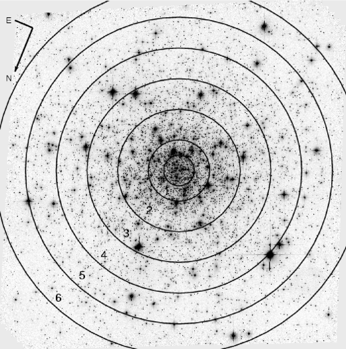
Figure 1: Negative image of the cluster NGC 2298 through the F606W band. The field spans $3\aas@@fstack{\prime}4$ on a side. The circles marked on the frame define the six annuli in which we have divided our photometry, as explained in Section 3.

2 Observations and data analysis

NGC 2298 was observed with the Advanced Camera for Surveys (ACS; see Ford et al. 2003; Pavlovsky et al. 2006) on board the HST on 2006, June 12 as part of the treasury programme entitled “An ACS Survey of Galactic Globular Clusters” (P.I. Ata Sarajedini). A series of five dithered exposures lasting 350 s each (plus an additional short exposure of 20 s duration) were collected through the F606W and F814W filters, for a total exposure time of 1770 s in each band. The telescope was pointed at the nominal centre of NGC 2298 at RA(J2000)$=06^{\rm h}48^{\rm m}59^{\rm s}5$ and DEC(J2000)$=-36^{\rm o}00\arcmin 30\arcsec$, corresponding to Galactic coordinates $l=245.6$ and $b=-16.0$. The field of view of the ACS Wide Field Channel, used for these observations, spans about $3\aas@@fstack{\prime}4$ on a side and reaches out to more than twice the cluster’s half-mass radius ($r_{\rm h}=0\aas@@fstack{\prime}78$; Harris 1996).

The raw data were retrieved from the HST archive after having been processed through the standard ACS pipeline calibration, which also took care of correcting the geometric distortion and calibrating the photometric zero point (Sirianni et al. 2005). The procedure also registered and combined the images in the same band. In Figure 1 we show a negative image of the final combined F606W frame.

Star detection and identification was done by running the automated IRAF daofind routine on the F606W band combined frame, with the detection threshold set at $10\,\sigma$ above the local background level. This conservative choice for the detection threshold stems from the fact that in this work we are not specifically interested in detecting the faintest possible stars, but rather in mapping as uniformly as possible low-mass MS stars throughout the cluster. While it would have been possible to push the detection threshold down to $\sim 5\,\sigma$, this would have also implied a higher degree of photometric incompleteness and, therefore, a less robust LF. On the other hand, owing to the large number of saturated stars in the frames, even with our $10\,\sigma$ detection threshold a careful inspection of all objects found by the automated routine is necessary, since point spread function (PSF) tendrils and artefacts can easily be misclassified as bona-fide stars. Fully or partly resolved objects, namely background galaxies, were also eliminated from the catalogue during this procedure. The final star list obtained in this way includes $11,350$ unresolved objects, comprising both cluster and field stars.

Except for the innermost $\sim 10\arcsec$ radius, which we did not study, crowding is not severe and stellar magnitudes can be accurately estimated with aperture photometry. We used the standard IRAF DAOPhot package (Stetson et al. 1987) and, following the core aperture photometry technique (De Marchi et al. 1993), we set the aperture radius to $0\aas@@fstack{\prime\prime}1$, while measuring the local background in an annulus extending from $0\aas@@fstack{\prime\prime}15$ to $0\aas@@fstack{\prime\prime}25$ around each object.

Since the PSF of the WFC varies considerably across the field of view (Sirianni et al. 2005), photometry based on PSF-fitting requires an accurate knowledge of the PSF. Aperture photometry, on the other hand, is less sensitive to the actual change of the PSF, provided that the aperture is large enough to accommodate the PSF changes (Sirianni et al. 2005). We have experimented with several choices for the aperture and background annulus and have selected the combination indicated above since it provides the least photometric scatter around the main sequence (MS) in the colour–magnitude diagram (CMD; on average $0.04$ mag).

Instrumental magnitudes were finally calibrated using the photometric zero points for the ACS VEGAMAG magnitude system (Sirianni et al. 2005). Our $10\,\sigma$ detection limits correspond to magnitudes $m_{\rm 606}\simeq 26.5$ and $m_{\rm 814}\simeq 25$, where the relative photometric error is $\la 0.05$ mag. The absolute photometric uncertainty is of the same order of magnitude, mainly due to the use of a small aperture, which implies a relatively large aperture correction. More sophisticated photometric techniques (e.g. Anderson & King 2004), which take into account the local variation of the PSF, might further reduce the overall uncertainty and the scatter along the MS in the CMD. However, the level of accuracy that we have reached is more than adequate for the purpose of understanding the broad properties of the stellar MF of NGC 2298. For this reason, we decided to also ignore the effects of the imperfect charge-transfer efficiency affecting ACS data (Sirianni et al. 2005), which contribute to broadening the MS in the CMD. None of the conclusions that we draw in this work are sensitive to this effect.

Figure 2: Colour–magnitude diagram of an area of $3\aas@@fstack{\prime}4\times 3\aas@@fstack{\prime}4$ around the centre of NGC 2298.

3 The colour–magnitude diagram

The CMD of the complete set of $11,350$ objects that we have detected is shown in Figure 2, where the cluster’s MS is clearly visible. At magnitudes brighter than $m_{\rm 814}\simeq 18.5$ the CMD reveal stars evolving off the MS (sub-giant branch), but their photometry is increasingly unreliable, due to saturation. Here we concentrate on the cluster’s MS, which is narrow and well defined from the turn-off at $m_{\rm 814}=18.8$, where the photometric error is small ($\sigma_{\rm 606}\simeq\sigma_{\rm 814}\simeq 0.01$), through to $m_{\rm 814}\simeq 25$, where the error on the magnitude grows to $\sigma_{\rm 606}\simeq\sigma_{\rm 814}\simeq 0.04$.

Owing to the relatively low Galactic latitude of NGC 2298 ($b=-16^{\circ}$), some field star contamination has to be expected in the CMD of Figure 2. This can be seen at $m_{\rm 814}\ga 22$, where an increasing number of objects appears on both sides of the MS, with colours too red or too blue for them to be bona-fide MS stars, given the typical magnitude uncertainty at this brightness ($\sigma_{\rm 606}\simeq\sigma_{\rm 814}\simeq 0.04$).

As a first attempt to roughly estimate the relevance of this contamination, we turned to the Galaxy model of Ratnatunga & Bahcall (1985), which predicts about 17 field stars per arcmin square towards the direction of NGC 2298 down to magnitude $V=27$, with about half of them in the range $24<V<27$. This would correspond to $\sim 200$ contaminating field stars in our field of view down to $V=27$, of which $\sim 100$ brighter than $V=24$. The CMD of Figure 2 has of order 3,950 stars with $m_{\rm 606}\geq 24$, before any correction for incompleteness, and there are approximately $7,400$ stars brighter than that magnitude. Therefore, it would seem perfectly unnecessary to take field star contamination into account.

On the other hand, since field star contamination affects more prominently the lower end of the MS, which is most relevant to our investigation, we decided to remove it at all magnitudes, following a statistical approach. To this aim, we made use of the colour information in the CMD and applied the $\sigma$-clipping criterion described by De Marchi & Paresce (1995) to identify the possible outliers. In practice, from the CMDs of Figure 2 we counted the objects in each $0.5$ mag bin and within $\pm 2.5$ times the colour standard deviation around the MS ridge line and rejected the rest as field objects. This procedure is iterative and at each step the colour of the ridge line and its associated standard deviation are recalculated. Convergence is reached, usually within a few iterations, when all stars whose colour differs from the average by more than $\pm 2.5$ times the MS standard deviation have been removed. In this way we identified about $320$ field stars, of which about $150$ fainter than $m_{\rm 606}\simeq 24$ (or $m_{\rm 814}\simeq 22$). These values are within a factor of two of those predicted by the model of Ratnatunga & Bahcall (1985) and as such are in surprisingly good agreement, given the large uncertainty affecting the Galaxy model of Bahcall & Soneira (1984) for $10^{\circ}<|b|<20^{\circ}$, due to the lack of direct observational calibration.

The number of putative field stars, determined with our procedure, is shown in Table 1 as a function of the magnitude, together with the average MS colour (ridge line) and associated standard deviation. We stress here that field stars account for an insignificant fraction ($\sim 3\,\%$) of the bona-fide MS stars and that, in each magnitude bin, their number is smaller than the statistical uncertainty associated with the counting process. In the following, we will consider only bona fide MS stars as defined in this way but, as will become clear in the rest of the paper, our determination of the MF of NGC 2298 would remain unchanged if we had decided to ignore field star contamination and treat all stars as cluster members.

Table 1: Average main sequence fiducial points, colour width and number of field stars.

$m_{\rm 814}$	$m_{\rm 606}-m_{\rm 814}$	$\sigma_{\rm 606-814}$	$N_{\rm F}$
18.75	0.592	0.035	12
19.25	0.608	0.035	20
19.75	0.642	0.035	28
20.25	0.692	0.037	24
20.75	0.765	0.041	22
21.25	0.850	0.043	27
21.75	0.952	0.050	29
22.25	1.057	0.050	27
22.75	1.152	0.050	23
23.25	1.223	0.050	29
23.75	1.274	0.061	36
24.25	1.332	0.079	25
24.75	1.385	0.097	15

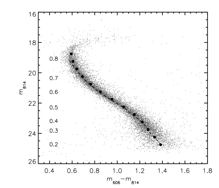
Figure 3: Main sequence ridge line of NGC 2298 (filled circles) compared with the theoretical isochrones of Baraffe et al. (1997; dashed line) for an age of 10 Gyr and metallicity $[M/H]=-1.5$, in the magnitude system of the ACS (see text).

Figure 3 shows, traced over the same CMD of Figure 2, the MS ridge line (filled circles) obtained by applying the sigma-clipping method explained above. The dashed line in the same figure corresponds to the theoretical isochrone computed by Baraffe et al. (1997) for a 10 Gyr old cluster with metallicity $[M/H]=-1.5$ and Helium content $Y=0.25$, as is appropriate for NGC 2298 (McWilliam, Geisler & Rich 1992; Testa et al. 2001). We have assumed a distance modulus $m-M=15.15$ and colour excess $E(B-V)=0.14$ from Harris (1996). The models of Baraffe et al. (1997) are calculated for the F606W and F814W filters of the WFPC2 camera, which do not exactly match those on board the ACS. The magnitude difference between the two cameras in the same band is a function of the effective temperature of the star (hence of its mass) and can be approximately estimated by means of the HST synthetic photometric package “Synphot” (Laidler et al. 2005). To calculate the correction factors, we have used synthetic atmosphere models from the ATLAS9 library of Kurucz (1993) with effective temperature and surface gravity matching those of the models of Baraffe et al. (1997). The resulting differences, in the F606W band, range from $0.028$ mag for stars of $0.8$ ${\rm M}_{\odot}$to $0.074$ mag for stars of $0.2$ ${\rm M}_{\odot}$. In the F814W band, the differences are smaller and range from $0.007$ mag to $0.036$ mag over the same mass range. The dashed line in Figure 3 shows the effect of translating the Baraffe et al. (1997) models to the ACS magnitude system, over the mass range $0.2-0.8$ ${\rm M}_{\odot}$(the mass points are indicated on the left-hand side). The agreement with the MS ridge line is very good and convinced us that we can use the translated models to convert magnitudes into masses.

4 The luminosity and mass function

The LF of MS stars is derived from the CMD of Figure 2 as part of the same sigma-clipping process that rejects field stars, since all objects that are not rejected are by definition bona-fide MS stars. Given the richness of the photometry and the wide field covered by the data, reaching out to more than twice the cluster’s half-mass radius ($r_{\rm h}=0\aas@@fstack{\prime}78$; Harris 1996), it is possible to study with accuracy the variation of the LF with radius. This is an essential step in securing a solid GMF.

To this aim, we have grouped our photometric catalogue to form a series of 6 concentric annuli, centered on the nominal cluster centre and expending out to $120\arcsec$, with a step of $20\arcsec$. Since the stellar density increases considerably towards the cluster’s centre, we did not consider the innermost $10\arcsec$ radius where the photometric completeness is very low due to the many bright stars. For simplicity, hereafter we refer to these regions as “rings” 1 through to 6, as marked in Figure 1. They contain, respectively, 1653, 2609, 3016, 2827, 1946, and 566 objects. Ring 3 is of particular importance, since it covers the region around the cluster’s half-mass radius, where the properties of the local MF are expected to be as close as possible to those of the global MF (Richer et al. 1991; De Marchi & Paresce 1995; De Marchi et al. 2000).

The large density gradient in the images implies that the completeness of the photometry is not uniform across the field. Incompleteness is due to crowding and to saturated stars, whose bright halo can mask possible faint objects in their vicinity, both more likely to affect substantially the central regions (see Figure 1). If ignored or corrected for in a uniform way across the whole image, by applying the same correction to all regions, these effects would bias the final results and mimic the presence of a high degree of mass segregation. For this reason, we conducted a series of artificial star experiments over the regions corresponding to each of the five individual annuli.

The artificial star tests were run on the combined images, in the F606W band (the same used for star detection). For each $0.5$ magnitude bin we carried out 10 trials by adding a fraction of 10 % of the total number of objects (see Section 2). The artificial images were then reduced with the same parameters used in the reduction of the scientific images so that we could assess the fraction of objects recovered by the procedure. The resulting photometric completeness is given in Table 2 for each region as a function of the $m_{\rm 814}$ magnitude.

Table 2: Photometric completeness $f$ in the six individual rings.

$m_{\rm 814}$	Ring 1	Ring 2	Ring 3	Ring 4	Ring 5	Ring 6
18.75	0.95	0.97	0.97	0.99	0.99	0.99
19.25	0.93	0.96	0.97	0.98	0.99	0.99
19.75	0.91	0.95	0.96	0.98	0.99	0.99
20.25	0.89	0.95	0.96	0.98	0.99	0.99
20.75	0.86	0.95	0.96	0.98	0.99	0.99
21.25	0.84	0.94	0.95	0.97	0.99	0.99
21.75	0.82	0.94	0.95	0.97	0.99	0.99
22.25	0.79	0.93	0.95	0.97	0.98	0.98
22.75	0.75	0.93	0.94	0.96	0.98	0.98
23.25	0.71	0.92	0.94	0.96	0.97	0.97
23.75	0.62	0.89	0.91	0.94	0.97	0.97
24.25	0.53	0.86	0.89	0.93	0.96	0.96
24.75	0.50	0.85	0.88	0.92	0.96	0.96

Figure 4: The circles are the LFs of the six rings, after correction for photometric incompleteness (see Table 2). The actual measurements from Table 3 are shifted vertically by an arbitrary amount to increase readability. The geometric average radius of each ring is indicated in arcmin to the left of each curve. The theoretical LFs that best fit the data are shown as solid lines. The index of their corresponding power-law MF is, from bottom to top, $\alpha=1.6,1.1,0.5,0.1,0$ and $-0.1$. A positive index means that the number of stars decreases with mass. All but the innermost LF reach down to $0.2$ ${\rm M}_{\odot}$. The dashed line is the LF measured near the half-mass radius of NGC 6397 by De Marchi et al. (2000), with arbitrary vertical normalisation.

Table 3: Luminosity functions measured in each of the six rings. For each region, the table gives, as a function of the $m_{\rm 814}$ magnitude, the number of stars per half-magnitude bin before ($N_{\rm o}$) and after ($N$) completeness correction and the uncertainty ($\sigma_{\rm N}$) on $N$.

	Ring 1			Ring 2			Ring 3			Ring 4			Ring 5			Ring 6
$m_{\rm 814}$	$N_{\rm o}$	$N$	$\sigma_{\rm N}$	$N_{\rm o}$	$N$	$\sigma_{\rm N}$	$N_{\rm o}$	$N$	$\sigma_{\rm N}$	$N_{\rm o}$	$N$	$\sigma_{\rm N}$	$N_{\rm o}$	$N$	$\sigma_{\rm N}$	$N_{\rm o}$	$N$	$\sigma_{\rm N}$
18.75	78	82	9	96	99	10	101	103	10	84	85	9	60	60	7	11	11	3
19.25	154	166	13	188	195	15	146	151	13	121	123	11	64	64	8	25	25	5
19.75	190	209	16	228	239	17	196	203	15	154	157	13	86	86	9	35	35	6
20.25	197	222	16	229	241	17	249	259	18	195	199	15	124	125	11	31	31	5
20.75	191	221	16	244	257	18	285	298	19	237	242	17	141	142	12	42	42	6
21.25	156	185	15	246	260	18	259	271	18	224	230	16	135	136	12	37	37	6
21.75	139	169	14	199	211	16	244	256	17	223	229	16	160	161	13	40	40	6
22.25	117	148	13	215	230	16	228	240	17	224	231	16	155	157	13	43	43	6
22.75	100	133	12	193	208	15	261	276	18	255	264	18	186	190	14	45	46	6
23.25	79	111	11	198	216	16	294	314	20	324	338	21	194	200	15	73	75	8
23.75	80	129	12	183	206	15	287	314	20	293	311	20	229	237	17	73	75	9
24.25	24	45	7	113	131	12	178	200	15	208	224	16	171	177	14	41	42	6
24.75	—	—	—	70	82	9	98	111	11	124	134	12	99	103	10	27	28	5

The LF of MS stars in each ring is shown graphically in Figure 4, in units of apparent and absolute magnitude in the F814W band. Table 3 gives the five LFs, before and after correction for photometric incompleteness, and the corresponding rms errors coming from the Poisson statistics of the counting process (only for the LF corrected for incompleteness). All values have been rounded off to the nearest integer. The LFs are remarkably flat, but a progressive steepening is evident with increasing radius. This trend is not the result of decreasing photometric completeness since only data-points with an original associated photometric completeness in excess of 85 % (50 % for Ring 1) are shown in Figure 4, as witnessed by Table 2.

It is instructive to compare the LF of Ring 3 (at the cluster’s half-mass radius) with that of NGC 6397, shown as a dashed line in Figure 4. Both are halo clusters with low metallicity ([Fe/H]$=-1.95$ for NGC 6397 and [Fe/H]$=-1.85$ for NGC 2298; Harris 1996), but while near the half-mass radius of NGC 6397 the number of stars per unit magnitude grows by a factor of about four from the turn-off luminosity to the LF peak at $M_{\rm 814}\simeq 8$ (King et al. 1998), for NGC 2298 it only changes by a factor of two. NGC 2298 is therefore seriously lacking low-mass stars with respect to NGC 6397.

Since the MS of NGC 2298 is well fitted by the theoretical isochrones of Baraffe et al. (1997), after conversion to the ACS photometric system (see Figure 3), we can use the associated mass–luminosity (M–L) relationships to convert magnitudes to masses. In order to keep observational errors clearly separated from theoretical uncertainties, we prefer to fold a model MF through the M–L relationship and compare the resulting model LF with the observations. The solid lines in Figure 4 are the theoretical LFs obtained by multiplying a simple power-law MF of the type $dM/dm\propto m^{\alpha}$ by the derivative of the M–L relation. Over the mass range ($0.2-0.8$ ${\rm M}_{\odot}$) spanned by these observations a simple power-law is a valid representation of the MF, although at lower masses the MF progressively departs from a power-law and this simplifying assumption is no longer a good representation of the mass distribution in GCs (PDM00; De Marchi, Paresce & Portegies Zwart 2005).

With the adopted M–L relation, a distance modulus $m-M=15.15$ and colour excess $E(B-V)=0.14$ (see Section 3), the best fitting local power-law slopes are $\alpha=1.6,1.1,0.5,0.1,0,-0.1$ respectively at $r=0\aas@@fstack{\prime}3,0\aas@@fstack{\prime}5,0\aas@@fstack{\prime}8,1\aas@@fstack{\prime}2,1\aas@@fstack{\prime}5,1\aas@@fstack{\prime}8$. The fact the value of the index is in almost all cases positive implies that the number of stars is decreasing with mass. With the notation used here, the canonical Salpeter IMF would have $\alpha=-2.3$. For comparison, over the same mass range spanned by the MF of Ring 3, the power-law index that best fits the MF of NGC 6397 is $\alpha\simeq-1.6$ (see dashed line in Figure 4) and that of the other 11 halo GCs in the sample studied by PDM00 is of the same order. It is, therefore, clear that NGC 2298 is surprisingly devoid of low-mass stars, at least out to over twice its half-mass radius.

5 The global mass function

Given the large spread of MF indices that we find, ranging over a dex, it is fair to wonder which of these MFs, if any, is representative of the mass distribution in the cluster as a whole. It is in principle possible (although not very likely, since the observations sample well more than half of the cluster’s population by mass), that a large number of low-mass stars is present in the cluster, but located beyond the radius covered by the these data. To clarify this issue, it is useful to study the dynamical state of NGC 2298 and investigate whether the observed MF variation with radius is consistent with the degree of mass segregation expected from energy equipartition due to two-body relaxation.

To this aim, we followed the approach outlined by Gunn & Griffin (1979). We employed the multi-mass Michie–King code originally developed by Meylan (1987, 1988) and later suitably modified by us (Pulone, De Marchi & Paresce 1999); De Marchi et al. 2000) for the general case of clusters with multiple LF measurements at various radii. Each model run is characterised by a MF in the form of a power-law with a variable index $\alpha$, and by four structural parameters describing, respectively, the scale radius ($r_{\rm c}$), the scale velocity ($v_{\rm s}$), the central value of the dimensionless gravitational potential $W_{\rm o}$, and the anisotropy radius ($r_{\rm a}$).

From the parameter space defined in this way, we selected those models that simultaneously fit both the observed surface brightness profile (SBP) and the central value of the velocity dispersion as given, respectively, by Trager et al. (1995) and Webbink (1985). However, while forcing a good fit to these observables constrains the values of $r_{\rm c}$, $v_{\rm s}$, $W_{\rm o}$, and $r_{\rm a}$, the MF can still take on a variety of shapes. To break this degeneracy, we impose the additional condition that the model LF agrees with that observed at all available locations simultaneously. This, in turn, sets very stringent constraints on the present GMF, i.e. on the MF of the cluster as a whole.

Figure 5: The LFs of Figure 4 (circles) are compared with those predicted by our multi-mass Michie–King model at various radii inside the cluster (dashed lines), for a GMF with index $\alpha=0.5$. The expected radial variation of the LF is fully consistent with the observations.

For practical purposes, the model GMF has been divided into sixteen different mass classes, covering main sequence stars, white dwarfs and heavy remnants, precisely as described in Pulone et al. (1999). We ran a large number of trials looking for a suitable shape of the GMF such that the local MFs implied by mass segregation would locally fit the observations. As explained in the previous section, in order to keep observational errors and theoretical uncertainties separate, we converted the model MFs to LFs, using the same M–L relation, distance modulus and colour excess of Figure 4, and compared those to the observations.

Our analysis shows that the set of model LFs that best fits all available observations simultaneously corresponds to a GMF index $\alpha=0.5$ for stars less massive than $0.8$ ${\rm M}_{\odot}$. At higher masses, we assume that the IMF had originally a power-law shape with index $\alpha=-2$, close to the Salpeter value $-2.3$. This parameter determines the fraction of heavy remnants in the cluster (white dwarfs, neutron stars and black holes), which we find to be of order $60\,\%$, and affects the overall distribution of the stars in all other classes of mass, to which the SBP is rather sensitive. We find that values of $\alpha$ larger or smaller than $-2$ give a progressively worse fit to the SBP, which becomes unacceptable for $\alpha>-1.5$ or $\alpha<-2.5$.

The best fit to the LFs is shown in Figure 5. The same model also reproduces remarkably well the SBP of Trager et al. (1995), as shown in Figure 6, and the value of the core radius that we obtain is $r_{\rm c}=18\arcsec$, in good agreement with the literature value $r_{\rm c}=20\arcsec$ of Harris (1996). We note here that in Figure 6 we compare to the data of Trager et al. (1995) the model SBP for stars of $0.8$ ${\rm M}_{\odot}$, i.e. turn-off and red giant stars, since these dominate the integrated light. Obviously, star of different masses have a different radial distribution, with the relative density at any location being governed by the relaxation process (King 1966). The cluster’s structural parameters and integrated luminosity derived from our best model are compared with their corresponding literature values in Table 4 and appear in rather good agreement with the latter.

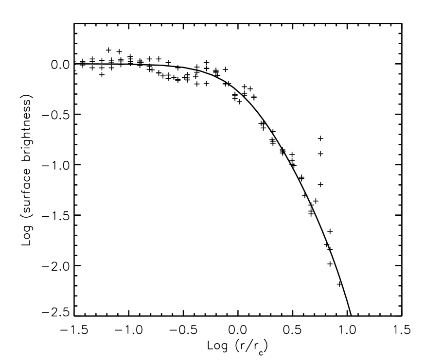
Figure 6: The surface brightness profile of NGC 2298 (crosses, from Trager et al. 1995) is well reproduced by our dynamical model (solid line). The observations are normalised to the central value of the best fitting profile as given by Trager et al. (1995).

Table 4: Cluster structural parameters for NGC 2298

Parameter	Fitted	Literature	Ref.
	value	value
core radius $r_{\rm c}$	$0\aas@@fstack{\prime}29$	$0\aas@@fstack{\prime}34$	$a$
tidal radius $r_{\rm t}$	$8\aas@@fstack{\prime}0$	$6\aas@@fstack{\prime}5$	$a$
half-mass radius $r_{\rm h}$	$1\aas@@fstack{\prime}2$	$0\aas@@fstack{\prime}8$	$a$
central vel. disp. $\sigma_{\rm o}$	$3.3$ km/s	$3.6$ km/s	$b$
total luminosity $M_{\rm V}$	$-6.3$	$-6.3$	$a$

$a$): Harris (1996)

$b$): Webbink (1985)

By design, also the central velocity dispersion predicted by the model matches the literature value (see Table 4), although the latter is not well constrained for NGC 2298. The value published by Webbink (1985), $\sigma_{\rm o}=3.6$ km/s, is not a direct measurement, but rather the result of a model. To our knowledge, the only recent radial velocity measurements in NGC 2298 are those by Geisler et al. (1995) of 9 red giant stars located between $1^{\prime}$ and $1\aas@@fstack{\prime}5$ from the cluster centre, or approximately at the half-mass radius. These measurements have an accuracy of $\sim 2$ km/s and their standard deviation is $3.7$ km/s. This value is in agreement with the estimate of Webbink (1985). It also agrees with the prediction of our model, which gives a velocity dispersion of $\sim 3$ km/s between $1^{\prime}$ and $1\aas@@fstack{\prime}5$ from the centre.

From $r_{\rm c}$, $\sigma_{\rm o}$ and $W_{\rm o}$ we derive the total cluster mass to be $5.1\times 10^{4}$ ${\rm M}_{\odot}$.

The good agreement between the observed radial variation of the LF and that predicted by the Michie–King model (Figure 5) implies that stars in NGC 2298 must be very close to a condition of equipartition, at least over the area covered by the observations. Sosin (1997) has shown that this is the case even if the phase space distribution function may not be the lowered-Maxwellian required by the Michie–King model (Michie & Bodenheimer 1963; King 1966). The half-mass relaxation time that our model indicates is $t_{\rm hm}=3.1$ Gyr, considerably shorter than GC ages (Krauss & Chaboyer 2003). As for the shape of the GMF, the index $\alpha=0.5$ implies that it is decreasing with mass. This confirms that the deficiency of low-mass stars inferred from Figure 4 is a general characteristic of NGC 2298 and not just the local effect of mass segregation. The excellent match between the GMF index $\alpha=0.5$ and that of the local MF measured near the half-mass radius (also $\alpha=0.5$) shows once more that the latter is an accurate approximation to the cluster’s GMF (Richer et al. 1991; De Marchi et al. 1995; De Marchi et al. 2000).

6 Discussion and conclusions

According to the classification of Zinn (1993), NGC 2298 is an old halo cluster by virtue of its low metallicity [Fe/H]$=-1.85$ (Harris 1996). The age of $\sim 12$ Gyr estimated by Testa et al. (2001) from the properties of horizontal branch stars is fully consistent with this classification. As indicated above, NGC 6397, another old halo cluster, has very similar metallicity [Fe/H]$=-1.95$. Its age is also similar: Gratton et al. (2003), using isochrone fitting to the MS, estimate $13.4\pm 0.8\pm 0.6$ Gyr and Richer et al. (2005), using the white dwarf cooling sequence, derive $\sim 12.7$ Gyr, in good agreement. It appears, therefore, logical to suppose that the two clusters were born with a similar IMF.

Their present GMFs, however, are quite different. As noted in Section 5, that of NGC 2298 is best described by a power-law with index $\alpha=0.5$ over the range $0.2-0.8$ ${\rm M}_{\odot}$. As for NGC 6397, although its GMF is more complex and is best represented by a log-normal distribution (PDM00) or by a tapered power-law (De Marchi et al. 2005), over the mass range $0.3-0.8$ ${\rm M}_{\odot}$  it is still well described by a simple power-law of index $\alpha=-1.6$ (De Marchi et al. 2000). Thus, the marked difference in their present GMF (PGMF) must be the result of dynamical evolution, namely the evaporation of stars via two-body relaxation, possibly enhanced by the effect of the Galactic tidal field (Aguilar, Hut & Ostriker 1988; Vesperini & Heggie 1997; Murali & Weinberg 1997; Gnedin & Ostriker 1997).

Since we have studied the present dynamical structure of both clusters (see Section 5 above and De Marchi et al. 2000), we can look for signs of a faster mass loss from NGC 2298. Both objects are in a condition of equipartition, as shown by the fact that the radial variation of their MFs resulting from mass segregation is well fitted by a simple multi-mass Michie–King model. They also have a similar total mass, namely $5.1\times 10^{4}$ ${\rm M}_{\odot}$  for NGC 2298 and $8.9\times 10^{4}$ ${\rm M}_{\odot}$  for NGC 6397 (De Marchi et al. 2000). We note here that both mass values come from a multi-mass Michie–King model and are based on measured velocity dispersions rather than by simple multiplication of the total cluster luminosity by an arbitrary $M/L$ ratio, as one too often finds in the literature. Their density, however, is rather different, as witnessed by the value of the central concentration parameter $c=\log(r_{\rm t}/r_{\rm c})$, which takes on the value of $1.3$ and $2.5$, respectively for NGC 2298 and NGC 6397 (Harris 1996).

In fact, the most outstanding dynamical difference between the two objects is that NGC 6397 appears to be in a more advanced evolutionary stage, since its high central concentration suggests that it has a post-collapse core (King, Sosin & Cool 1995). This, however, should not imply a higher mass-loss rate for NGC 2298. In fact, one would expect clusters in a more advanced dynamical phase (i.e. those with post-collapse cores) to have lost more low-mass stars via the evaporation process caused by two-body relaxation (Vesperini & Heggie 1997).

In any case, the evaporation process alone appears to be insufficient to account for the depletion of low mass stars in NGC 2298 and, as such, it may not be the primary cause of mass loss from this cluster. We show this with a simple “order-of-magnitude” calculation. If we assume that NGC 2298 and NGC 6397 were born with the same IMF and, following the conclusions of PDM00, that the PGMF of NGC 6397 is substantially coincident with its IMF, then a simple integration of the difference between the two PGMFs shows that NGC 2298 must have lost about 85 % of its original mass in the course of its life. This would imply an average evaporation rate of $\sim 2\times 10^{-5}$ ${\rm M}_{\odot}$/yr.

Evaporation takes place on a timescale considerably longer than relaxation, at least one order of magnitude longer (Spitzer 1987). Based on the value of the half-mass relaxation time that we find ($t_{\rm rh}\simeq 3$ Gyr), we estimate an evaporation timescale $t_{\rm evap}\ga 30$ Gyr, for the present mass and structure of the cluster, corresponding to an average evaporation rate of $\la 2\times 10^{-6}$ ${\rm M}_{\odot}$/yr, or an order of magnitude less than that required to deplete the GMF of NGC 2298 at the low mass end to the level observed today. Considering that $t_{\rm evap}$ scales with the total mass of the cluster, and was therefore longer in the past, it appears unlikely that the internal evaporation process alone may have removed a conspicuous fraction of NGC 2298’s original mass in the $\sim 13$ Gyr of its life.

Clearly, however, evaporation is not the only process that can remove stars from a GC. Clusters with orbits crossing the Galactic plane or venturing close to the Galactic centre undergo compressive heating, respectively via disc and bulge shocking, which can have a much stronger effect than evaporation on the loss of stars, depending on the orbit (Aguilar, Hut & Ostriker 1988; Gnedin & Ostriker 1997; Dinescu et al. 1999b).

Orbital parameters have been determined for both clusters via proper motion and radial velocity measurements (Dinescu et al. 1999a, 1999b; Cudworth & Hanson 1993; Dauphole et al. 1996). Here a remarkable difference exists between NGC 6397, which occupies a low-eccentricity orbit ranging between 3 and 6 kpc from the Galactic centre, and NGC 2298, which has a very eccentric orbit with perigalactic and apogalactic distances of respectively 2 and 15 kpc. The maximum distance from the Galactic plane for NGC 6397 is $1.5$ kpc, whereas NGC 2298 reaches as far as $\sim 7$ kpc. The orbital periods are 143 and 304 Myr, respectively (Dinescu et al. 1999b). It appears that, for most of its orbit, NGC 2298 is too far removed from the disc and bulge of the Galaxy for the compressive heating mentioned above to be a serious threat for the cluster. Indeed, on the basis of these space motion parameters, Gnedin & Ostriker (1997), Dinescu et al. (1999b) and Baumgardt & Makino (2003) conclude that evaporation is the dominant cause of disruption for both clusters. Quite surprisingly, the rate of disruption of NGC 6397 is twice as high as that of NGC 2298, according to these authors. This is not compatible with the observations, if the clusters were born with a similar IMF.

The careful reader will not have missed that it is also entirely possible that our assumption is ill founded and that NGC 2298 and NGC 6397 were not born with the same IMF, even though they have similar age and metallicity. In fact, given the evidence above and taking the model predictions at face value, one would be tempted to conclude that NGC 2298 was born with a considerably flatter IMF (i.e. with a smaller proportion of low-mass stars) than NGC 6397 or any other known halo cluster (PDM00). As explained in De Marchi, Paresce & Pulone (2007), however, the existence of a trend between the central concentration of a cluster and its GMF index argues against this hypothesis. Denser clusters are found to have a systematically steeper GMF than loose clusters and since it is hard to imagine that the star formation process could know about the final dynamical structure of the forming cluster, the observed trend is most likely the result of dynamical evolution, i.e. low-mass star evaporation and tidal stripping. Therefore, the origin of the large difference between the GMFs of NGC 6397 and NGC 2298 will have to be searched in the details of the past dynamical histories of these two objects, which are still largely unknown.

To be sure, models of how GCs interact with the Galaxy are rather uncertain and their predictions have to be taken with great care. Uncertainties on the orbit of individual clusters, determined from their current proper motion and radial velocity, can be large. Furthermore, the actual distribution of the mass in the Galaxy has never been directly measured and models must be used instead (e.g. Bahcall, Soneira & Schmidt 1983; Ostriker & Caldwell 1985; Johnston, Spergel & Hernquist 1995), which are affected by unavoidable uncertainties. Therefore, while the predictions of how GCs interact with the Galaxy may well be valid in a statistical sense when it comes to describing the global properties of the GC system, their applicability to individual objects is not guaranteed (De Marchi et al. 2006). For instance, the perigalactic distance of NGC 2298 is known with considerable uncertainty, $R_{\rm p}=2.1\pm 1.6$ kpc, compared to NGC 6397 for which $R_{\rm p}=3.1\pm 0.2$ kpc (Dinescu et al. 1999a). Since the rate of disruption due to bulge shocking scales with $R_{\rm p}^{-4}$, if $R_{\rm p}$ for NGC 2298 were to decrease by a factor of 2 or 3 (compatible with the present uncertainty), bulge shocking could become the dominant mass loss mechanism and explain, at least qualitatively, the difference with the PGMF of NGC 6397. Unfortunately, this situation will not improve until more accurate astrometric information becomes available for a sizeable number of GCs and a better understanding of the mass distribution in the bulge is secured. It is expected that this will be possible with the advent of Gaia.

- (1) Aguilar, L., Hut, P., Ostriker, J. 1988, ApJ, 335, 720
- (2) Anderson, J., King, I. 2004, Advanced Camera for Surveys Instrument Science Report 15-04, (Baltimore: STScI)
- (3) Andreuzzi, G., De Marchi, G., Ferraro, F. R., Paresce, F., Pulone, L., Buonanno, R. 2001, A&A, 372, 851
- (4) Bahcall, J., Soneira, R. 1984, ApJS, 55, 67
- (5) Bahcall, J., Soneira, R., Schmidt, M. 1983, ApJ, 265, 730
- (6) Baraffe, I., Chabrier, G., Allard, F., Hauschildt, P. 1997, A&A, 327, 1054
- (7) Baumgardt, H., Makino, J. 2003, MNRAS, 341, 247
- (8) Cudworth, K., Hanson, R. 1993, AJ, 105, 168
- (9) Dauphole, B., Geffret, M., Colin, J., Ducourant, C., Odenkirchen, M., Tucholke, H. 1996, A&A, 313, 119
- (10) De Marchi, G., Leibundgut, B., Paresce, F., Pulone, L. 1999, A&A 343, 9L
- (11) De Marchi, G., Paresce, F. 1995, A&A, 304, 202
- (12) De Marchi, G., Paresce, F., Portegies Zwart, S. 2005, in The initial mass function 50 years later, ASSL 327, Eds. E. Corbelli, F. Palla, H. Zinnecker (Dordrecht: Springer), 77.
- (13) De Marchi, G., Paresce, F., Pulone, L. 2000, ApJ, 530, 342
- (14) De Marchi, G., Paresce, F., Pulone, L. 2007, ApJL, submitted
- (15) De Marchi, G., Pulone, L., Paresce, F. 2006, A&A, 449, 161
- (16) De Marchi, G., Nota, A., Leitherer, C., Ragazzoni, R., Barbieri, C. 1993, ApJ, 419, 658
- (17) Dinescu, D., van Altena, W. F., Girard, T., Lopez, C. 1999a, AJ, 117, 277
- (18) Dinescu, D., Girard, T., van Altena, W. 1999b, AJ, 117, 1792
- (19) Ford, H., et al. 2003, SPIE, 4854, 81
- (20) Geisler, D., Piatti, A., Claria, J., Minniti, D. 1995, AJ, 109, 605
- (21) Gnedin, O., Ostriker, J. 1997, ApJ, 474, 223
- (22) Gratton, R., Bragaglia, A., Carretta, E., Clementini, G., Desidera, S., Grundahl, F., Lucatello, S. 2003, A&A, 408, 529
- (23) Gunn, J., Griffin, R. 1979, AJ, 84, 752
- (24) Harris, W. 1996, AJ 112, 1487 (revision 2003)
- (25) Hénon, M. 1961, AnAp, 24, 369
- (26) Hénon, M. 1965, AnAp, 28, 62
- (27) Johnston, K., Spergel, D., Hernquist, L. 1995, ApJ, 451, 598
- (28) King, I. 1966, AJ, 71, 64
- (29) King, I., Anderson, J., Cool, A., Piotto, G. 1998, ApJ, 492, L37
- (30) King, I., Sosin, C., Cool, A. 1995, ApJ, 452, L33
- (31) Koch, A., Grebel. E., Odenkirchen, M., Martinez–Delgado, D., Caldwell, J. 2004, AJ, 128, 2274
- (32) Krauss, L., Chaboyer, B. 2003, Science, 299, 65
- (33) Kurucz, R. L. 1993, in Peculiar versus Normal Phenomena in A-type and Related Stars, ASP Conf. Ser. 44, 87
- (34) Laidler et al. 2005, Synphot User’s Guide, Version 5.0 (Baltimore: STScI)
- (35) Meylan, G. 1987, A&A 184, 144
- (36) Meylan, G. 1988, A&A 191, 215
- (37) McWilliam, A., Geisler, D., Rich, R. 1992, PASP, 104, 1193
- (38) Michie, R., Bodenheimer, P. 1963, MNRAS, 126, 269
- (39) Murali, C., Weinberg, M. 1997, MNRAS, 288, 749
- (40) Ostriker, J., Caldwell, J. 1983, in Kinematics, Dynamics and Structure of the Milky Way, ed. W. L. H. Shuter (Dordrecht: Reidel), 249
- (41) Paresce, F., De Marchi, G. 2000, ApJ, 534, 870
- (42) Pavlovsky, C., et al. 2006, ACS Instrument Handbook, Version 7.0, (Baltimore: STScI)
- (43) Pulone, L., De Marchi, G., Paresce, F. 1999, A&A, 342, 440
- (44) Pulone, L., De Marchi, G., Paresce, F. 2007, A&A, in preparation
- (45) Ratnatunga, K.U., Bahcall, J.N. 1985, ApJS, 59, 63
- (46) Richer, H. et al. 2005, BAAS, 37, 1373
- (47) Richer, H., Fahlman, G., Buonanno, R., Fusi Pecci, F., Searle, L., Thompson, I. 1991 381, 147
- (48) Sirianni, M., et al. 2005, PASP, 117, 1049
- (49) Sosin, C. 1997, AJ, 114, 1517
- (50) Spitzer, L. 1987, (Princeton: Princeton University Press)
- (51) Stetson, P. 1987, PASP, 99, 191
- (52) Testa, V., Corsi, C., Andreuzzi, G., Iannicola, G., Marconi, G., Piersimoni, A., Buonanno, R. 2001, AJ, 121, 916
- (53) Trager, S., King, I., Djorgovski, S. 1995, AJ, 109, 1912
- (54) Vesperini, E., Heggie, D. 1997, MNRAS, 289, 898
- (55) Webbink, F. 1985, in Dynamics of star clusters, IAU Symp. 113 (Dordrecht: Reidel), 541
- (56) Zinn, R. 1993, in The Globular Cluster-Galaxy Connection, ASP Conf. Ser. 48, 38