XMM-Newton study of $0.012<z<0.024$ groups. I: Overview of the IGM thermodynamics.

Abstract

We study the thermodynamic properties of the hot gas in a sample of groups in the 0.012–0.024 redshift range, using XMM-Newton observations. We present measurements of temperature, entropy, pressure and iron abundance. Non-parametric fits are used to derive the mean properties of the sample and to study dispersion in the values of entropy and pressure. The scaling of the entropy at $0.2r_{500}$ matches well the results of Ponman et al. (2003). However, compared to cool clusters, the groups in our sample reveal larger entropy at inner radii and a substantially flatter slope in the entropy in the outskirts, compared to both the prediction of pure gravitational heating and to observations of clusters. This difference corresponds to the systematically flatter group surface brightness profiles, reported previously. The scaled pressure profiles can be well approximated with a Sérsic model with $n=4$. We find that groups exhibit a systematically larger dispersion in pressure, compared to clusters of galaxies, while the dispersion in entropy is similar.

1 Introduction

Use of clusters of galaxies in cosmological studies, requires a relation between the observed properties of the systems, such as X-ray luminosity, ICM temperature and the total mass of the system. Understanding this relation and its evolution with the redshift is therefore one of the key research focuses of modern astrophysics (e.g. Majumdar & Mohr 2004). Early observations have already demonstrated the importance of processes related to the physics of baryons in defining the observational appearance of clusters, and in particular on their low-mass end – groups of galaxies (e.g. Ponman et al. 1999). Currently, theoretical interpretation of the observed properties of groups and clusters of galaxies involves an interplay between the cooling and resulting star-formation and feedback (Borgani et al. 2001; Finoguenov et al. 2003; Voit et al. 2003; Kay et al. 2004). The complexity of the feedback schemes and variations in the feedback efficiency, given by IMF as well as AGN activity (e.g. Springel & Hernquist 2003), points to the importance of observations. In particular, observations of the cores of groups and clusters of galaxies are critical to understand the effects of cooling (Voit et al. 2001). Finoguenov et al. (2002) demonstrated that outskirts of groups and cool clusters also deviate from the expectations of gravitational heating, and cannot be explained by the effects of cooling. The challenging energetics of the observed effect, requires a very efficient feedback scheme, and the currently favoured mechanism invokes amplification of the entropy of the accreting gas by the shock heating – so called “smooth accretion” (Ponman et al. 2003; Voit et al. 2003; Voit & Ponman 2003; Borgani et al. 2005).

The large grasp of XMM-Newton provides us with new possibilities to test scenarios of group formation – in particular, the link between the state of the gas and the structure in X-ray images. Our idea here is quite straight-forward; since mergers are examples of lumpy accretion, post-merger groups should have on average lower entropy, compared to systems where the bulk of the material has been added through slow accretion. Thus, using two dimensional analysis of XMM-Newton data, combined with standard analysis using annuli, with limiting radii increasing logarithmically, we can both infer the state of the gas with unprecedented precision and provide an explanation of the observed trend by studying substructure. We also examine the dynamic state of the galaxies in these groups, to provide independent evidence.

At the moment there is no large purely X-ray selected sample of local groups of galaxies. For example, only a few objects, Fornax cluster, MKW4, NGC4636, NGC1550 and NGC5044 are present in the HIFLUGS, a complete all-sky sample of brightest groups and clusters of galaxies (Reiprich & Böhringer 2002). Most present-day samples of groups are based on the X-ray follow-up of the optical surveys (e.g. Mahdavi et al. 2000; Mulchaey et al. 2003). For this study we have primarily selected the groups primarily from Mulchaey et al. (2003) with publicly available XMM-Newton (Jansen et al. 2001) observations. Mulchaey list is based on the cross-correlating the ROSAT observation log with the positions of optically-selected groups in the catalogs of Huchra & Geller (1982), Geller & Huchra (1983), Maia et al. (1989), Nolthenius (1993) and Garcia (1993). While these catalogs also include richer galaxy systems (i.e. clusters), the Mulchaey list only includes systems with velocity dispersions less than 600 km/s or an intragroup medium temperature less than 2 keV.

A total of 25 systems observed by XMM-Newton have been selected, and further divided onto two samples covering the redshift ranges 0.004–0.012 and 0.012–0.024. The low-redshift sample is discussed in Finoguenov et al. (2006), while here we concentrate on the high redshift sample. Although our sample is not statistically complete, it has been shown by Finoguenov et al. (2006) that both XMM-Newton follow-up and the selection of the groups by Mulchaey et al. (2003) appear representative. We further increase our $z=$0.012–0.024 sample by addition of two groups, HCG51 and Pavo, which were not in Mulchaey’s sample (there has been no ROSAT PSPC observations of those two groups), but lie in the same redshift range.

An important difference between our ‘low’ and ‘high’ redshift subsamples consists in the different coverage of the group emission. While in the low-redshift sample, we concentrate on the properties of the central brightest group galaxies (BGGs), with the high-redshift sample typical scales resolved correspond to the transition zone between the BGG and the group. As the Mulchaey list is flux-limited, the typical luminosity of the high-redshift subsample is $10^{42}$ ergs s^-1, i.e. we look at bona fide groups, where the total X-ray flux is dominated by the group emission, while the origin of the hot gas is a specific aspect of the low-z subsample. In present sample, we have, however, included a few examples (e.g. HCG92), where strong galaxy interactions result in the high X-ray luminosity.

The present paper (Paper I) presents an analysis of the radial and 2-dimensional structure of the hot gas properties for the sample. The paper is organized as follows: §2 describes the analysis of the XMM-Newton observations; §3 outlines the average properties of the sample and dispersion around the mean trends; §4 describes each group of the sample individually; §5 concludes the paper.

Paper II (Osmond et al. 2006) is concerned with classifying the groups, on the basis of their gas properties, and looking at the relationship between different properties. Finally, a study of temperature and element abundance profiles using the Chandra observations of 15 groups with 6 overlapping with the current sample are reported in Rasmussen et al. (2006). It turns out that the Chandra sample is dominated by the cool core systems, which results in some differences in the reported mean trends. However for systems in common the results agree well.

2 Data

Tab.1 details the observations, listing the name of the group (column 1), the assigned XMM archival name (2), net Epic-pn exposure after removal of flaring episodes (3), pn filter used (4), needed for instrumental response as well as background estimates, XMM-Newton revolution number (5), useful assessment to the secular evolution of the instrumental background, pn frame time (6), which determines the fraction of out-of-time events.

Table 1: Log of the XMM Epic-pn observations of groups.

Name	Obs.	net	pn	XMM	frame
	ID	exp.	Filter	Orbit	time
		ksec			ms
3C449	0002970101	16.1	Medium	367	73
HCG 92	0021140201	30.1	Thin	366	73
Pavo	0022340101	9.1	Thin	423	73
HCG 42	0041180301	16.4	Medium	358	73
HCG 68	0041180401	16.3	Thick	454	73
NGC 5171	0041180801	13.2	Medium	377	199
HCG 15	0052140301	22.9	Thin	383	199
NGC 507	0080540101	25.9	Thin	202	199
NGC 4073	0093060101	9.4	Medium	373	199
NGC 4325	0108860101	14.8	Thin	191	73
NGC 2563	0108860501	15.9	Medium	339	73
NGC 533	0109860101	28.8	Thin	195	199
HCG51	0112270301	5.4	Thin	363	199
HCG 62	0112270701	8.1	Medium	568	199

Initial steps of data reduction are similar to the procedure described in Zhang et al. (2003), Finoguenov et al. (2003). As most of the observations analyzed here were performed using a short integration frame time for pn, it is important to remove the out-of-time events from imaging and spectral analysis. We used the standard product of epchain SAS task to produce the simulated OOTE file for all the observations and scale it by the fraction of the OOTE expected for the frame exposure time, as specified in Tab.1. For further details of XMM-Newton processing we refer the reader to http://wave.xray.mpe.mpg.de/xmm/cookbook/general page.

The analysis consists of two parts: first, revealing the structure in the surface brightness and temperature maps and second, verifying it through the spectral analysis. The first part consists in producing temperature estimates, based on the calibrated wavelet prefiltered hardness ratio maps and producing the projected pressure and entropy maps. Wavelet filtering (Vikhlinin et al. 1998) is used to find the structure and control its significance.

The second, spectroscopy part of the analysis, uses the mask file, created based on the results of both hardness ratio and surface brightness analysis described above. First application of this technique is presented in Finoguenov et al. (2003).

The approach to the analysis of the sample is as follows. Taking the directly observed image we divide it along the contours of surface brightness. For a symmetrical system, the result of this procedure will be annuli. For a system in hydrostatic equilibrium, and neglecting the effect of Fe abundance variations on the emission, such selection alone is sufficient to remove possible temperature mixing (the X-ray theorem, Buote & Canizares 1994, which although strictly valid in 3D, could be shown to result in a symmetry in a projection onto the observer’s plane for a single triaxial potential; the case of multiple subhalos will, however, suffer from projection effects). Next, we study the hardness ratio map, which is sensitive to temperature variations, allowing us to avoid mixing multiple temperature components in a blind spectral extraction. In combination with the first step, we are looking for deviations from hydrostatic equilibrium, or a presence of subhalos. We also build the projected entropy and pressure maps using an image and the hardness ratio map. Although this way of map construction suffers from a number of degeneracies, with metalicity-density being the strongest (a significant fraction of the group emission is due to the line emission), these maps indicate the regions of primary interest for detailed spectroscopic analysis, in which most of the degeneracies are removed. In general, the entropy should monotonically increase with the increasing radius, while the pressure should decrease.

The spectral analysis was performed using a single-temperature APEC plasma code with solar abundance pattern. Absorption was fixed at the galactic value, reported in Tab.2. In this work we employ a very detailed modeling of the background. First we consider the outermost part of the detector in respect to the group centre, in order to estimate the instrumental background. We subtract the background accumulation in order to remove most of the background and later look for the residuals. In our analysis we used the Read & Ponman (2003) background accumulation for the medium filter, XMM observation of CDFS (Streblyanska et al. 2006; Finoguenov in prep.) for the observations performed with the thin filter and an accumulation by Rossetti et al. (2005) for the thick filter. We use 0.45–7.5 and 9.5–12 keV bands and test the presence of the following components: hard instrumental background, having a slope of around 0. This background dominates at energies above 5 keV. Such a component is found in observations 0041180301 and 0041180801. Another component has a steeper index, 1–3, and is associated with the soft proton component. Such a component was added to the background for observations 0041180301, 0041180801 and 0112270301. Our analysis demonstrated that the scaling of these components, in particular the soft proton component, is somewhat more complicated than equal flux per detector area, we left the normalizations of these components free. We point out that an advantage of working with low-redshift groups, compared to clusters, is that group emission from a $\sim$1 keV thermal plasma is very different from the power law shape of the background.

Once the background components are estimated, we switch to the narrow energy band, 0.45–3 keV for fitting the source. We also consider adding a thermal component with a fixed temperature of 0.2 keV to account for the possible variation in the galactic foreground emission. This component was found to be significant in observations 0021140201 (HCG 92), 0022340101 (Pavo), 0041180801 (NGC 5171), 0108860101 (NGC 4325) and 0112270701 (HCG 51). In 0041180801, the temperature of this component was significantly higher, $0.35\pm 0.04$ keV. In the spectral analysis we group the channels to achieve 30 counts per bin, allowing us to apply $\chi^{2}$ fitting. All identified point sources were excised from the spectral extraction.

In calculating the local gas properties, we perform an estimate of the projection length of each analyzed region to obtain actual gas properties at these locations, as described at length in Henry et al. (2004) and Mahdavi et al. (2005). Since we do not perform a deprojection of the spectra, to reduce the importance of the projection effects we discard regions having a ratio of the minimal to the maximal distance from the centre of the group of values exceeding 0.8. The centre of a group is taken at the peak of the extended X-ray emission.

3 Average properties of the sample

We start this section by examining the mean trends seen in the data, comparing to previous results and then looking at the individual properties of the groups, where we identify the underlying cause for deviation of individual systems from the mean trend.

Table 2 lists the known properties of the groups. Column (1) identifies the system, (2) gives the value of galactic absorption towards the group (in spectral fitting we freeze the value of the absorbing column to this value), (3) redshift of the group, (4) velocity dispersion of the group galaxies, calculated as in Osmond & Ponman (2004), (5) optical luminosity of the group and separately of brightest group galaxy from Osmond & Ponman (2004), (6-7) temperature in the range $0.1-0.3r_{500}$ used for scaling ($T_{w}$), and estimate of $r_{500}$, obtained iteratively. The $r_{500}$ (radius within which the mean density is 500 times the critical value) is calculated as $r_{500}=0.391{\rm Mpc}\times(kT_{w}/{\rm keV})^{0.63}h_{70}^{-1}$ using the M–T relation (Pacaud, F. 2005, private communication) rederived from the Finoguenov et al. (2001) using an orthogonal regression and correcting the masses to $h_{70}$ and a LCDM cosmology. The $h(z)=(\Omega_{M}(1+z)^{3}+\Omega_{\Lambda})^{1/2}$ correction, is negligible for this sample and has not been applied. The suggested modified entropy scaling goes as $S\propto T_{w}^{2/3}$ (Ponman et al. 2003), which corresponds to a scaling of pressure $P\propto T_{w}^{3/2}$.

Table 2: Basic properties of groups.

Group     $N_{H}$		z	$\sigma_{group}$	$L_{B}$ (BGG)	kTw	$r_{500}$
$10^{20}$ cm-2			km/s	$10^{10}L_{\odot}$	keV	kpc
3C449	11.8	0.0171	$335\pm 112$	7.8 (2.24)	$1.28\pm 0.02$	453
HCG92	8.03	0.0221	$467\pm 176$	11.5 (3.31)	$0.79\pm 0.24$	334
Pavo	5.18	0.0134	$440\pm 96$	28.1 (8.84)	$0.77\pm 0.12$	330
HCG42	4.78	0.0132	$282\pm 43$	21.3 (8.91)	$0.75\pm 0.19$	324
HCG68	0.97	0.0078	$191\pm 68$	25.7 (4.37)	$0.69\pm 0.09$	308
NGC5171	1.93	0.0231	$494\pm 99$	19.1 (5.75)	$1.21\pm 0.05$	436
HCG15	3.20	0.0225	$404\pm 122$	7.1 (1.82)	$0.62\pm 0.04$	286
NGC507	5.24	0.0165	$580\pm 94$	48.8 (4.05)	$1.34\pm 0.01$	467
NGC4073	1.89	0.0199	$565\pm 72$	50.1 (15.5)	$1.87\pm 0.05$	575
NGC4325	2.23	0.0257	$376\pm 70$	11.5 (4.07)	$1.01\pm 0.01$	389
NGC2563	4.23	0.0149	$384\pm 49$	28.2 (4.27)	$1.31\pm 0.05$	460
NGC533	3.10	0.0185	$439\pm 60$	33.1 (9.77)	$1.26\pm 0.01$	448
HCG51	1.27	0.0265	$546\pm 151$	17.4 (3.59)	$1.16\pm 0.13$	424
HCG62	3.01	0.0145	$418\pm 51$	31.6 (3.47)	$1.06\pm 0.02$	403

Tables 5–5 present the characteristics of the groups obtained by mass-averaging of the observed spectroscopic components separated using the following radial bins: $<0.1r_{500}$, $0.1-0.3r_{500}$, $0.3-0.7r_{500}$. Col. (1) identifies the group, (2) reports the temperature in keV, (3) iron abundance as a fraction of the photospheric solar value of Anders & Grevesse (1989), (4) entropy, (5) pressure.

Table 3: Properties of groups within $0.1r_{500}$.

Name	kT	Z	S	P
	keV	$Z_{\odot}$	keV cm2	$10^{-12}$ dyne cm-2
3C449	$1.38\pm 0.02$	$0.33\pm 0.03$	$61.\pm 1.8$	$7.48\pm 0.30$
HCG92	$0.69\pm 0.05$	$0.22\pm 0.04$	$28.\pm 4.1$	$6.20\pm 0.77$
Pavo	$0.98\pm 0.08$	$0.25\pm 0.07$	$54.\pm 6.2$	$4.23\pm 0.50$
HCG42	$0.81\pm 0.07$	$0.30\pm 0.03$	$49.\pm 6.6$	$3.01\pm 0.39$
HCG68	$0.66\pm 0.02$	$0.18\pm 0.04$	$80.\pm 10.2$	$0.88\pm 0.14$
NGC5171	$1.55\pm 0.10$	$0.21\pm 0.09$	$111.\pm 10.2$	$4.46\pm 0.47$
HCG15	$0.66\pm 0.13$	$0.01\pm 0.02$	$34.\pm 8.2$	$2.58\pm 0.72$
NGC507	$1.27\pm 0.01$	$0.58\pm 0.02$	$42.\pm 0.6$	$11.06\pm 0.22$
NGC4073	$1.96\pm 0.04$	$0.82\pm 0.07$	$70.\pm 2.1$	$15.59\pm 0.52$
NGC4325	$0.94\pm 0.01$	$0.53\pm 0.06$	$24.\pm 1.3$	$11.49\pm 0.93$
NGC2563	$1.52\pm 0.04$	$0.44\pm 0.09$	$99.\pm 6.0$	$4.87\pm 0.39$
NGC533	$1.32\pm 0.01$	$0.50\pm 0.03$	$70.\pm 1.6$	$5.68\pm 0.18$
HCG51	$1.18\pm 0.15$	$0.59\pm 0.06$	$92.\pm 19.9$	$2.99\pm 0.59$
HCG62	$1.13\pm 0.02$	$0.37\pm 0.04$	$46.\pm 2.0$	$7.46\pm 0.40$

Table 4: Properties of groups between $0.1r_{500}$ and $0.3r_{500}$.

Name	kT	Z	S	P
	keV	$Z_{\odot}$	keV cm2	$10^{-12}$ dyne cm-2
3C449	$1.05\pm 0.02$	$0.09\pm 0.01$	$112\pm 3$	$1.48\pm 0.04$
HCG92	$0.78\pm 0.30$	$0.50\pm 0.93$	$251\pm 143$	$0.21\pm 0.16$
Pavo	$0.66\pm 0.08$	$0.36\pm 0.06$	$106\pm 19$	$0.51\pm 0.10$
HCG42	$0.75\pm 0.19$	$0.23\pm 0.06$	$169\pm 63$	$0.37\pm 0.12$
HCG68	$0.69\pm 0.09$	$0.50\pm 2.06$	$200\pm 31$	$0.22\pm 0.04$
NGC5171	$1.21\pm 0.05$	$0.17\pm 0.04$	$158\pm 10$	$1.30\pm 0.11$
HCG15	$0.85\pm 0.08$	$0.05\pm 0.02$	$81\pm 10$	$1.48\pm 0.24$
NGC507	$1.34\pm 0.01$	$0.33\pm 0.01$	$134\pm 2$	$2.21\pm 0.03$
NGC4073	$1.75\pm 0.03$	$0.26\pm 0.02$	$176\pm 3$	$2.90\pm 0.05$
NGC4325	$0.97\pm 0.01$	$0.39\pm 0.04$	$122\pm 5$	$1.09\pm 0.07$
NGC2563	$1.31\pm 0.05$	$0.23\pm 0.03$	$192\pm 11$	$1.20\pm 0.07$
NGC533	$1.26\pm 0.01$	$0.32\pm 0.02$	$140\pm 3$	$1.72\pm 0.06$
HCG51	$1.16\pm 0.13$	$0.59\pm 0.06$	$186\pm 30$	$0.92\pm 0.19$
HCG62	$1.06\pm 0.02$	$0.08\pm 0.01$	$107\pm 3$	$1.60\pm 0.05$

Table 5: Properties of groups between $0.3r_{500}$ and $0.7r_{500}$.

Name	kT	Z	S	P
	keV	$Z_{\odot}$	keV cm2	$10^{-12}$ dyne cm-2
3C449	$0.67\pm 0.04$	$0.04\pm 0.01$	$117.\pm 10.5$	$0.47\pm 0.05$
Pavo	$0.56\pm 0.10$	$0.21\pm 0.06$	$114.\pm 35.0$	$0.33\pm 0.09$
HCG42	$0.75\pm 0.48$	$0.20\pm 0.11$	$213.\pm 156.2$	$0.25\pm 0.20$
NGC5171	$0.98\pm 0.12$	$0.30\pm 0.13$	$475.\pm 257.1$	$0.22\pm 0.08$
NGC507	$1.07\pm 0.01$	$0.31\pm 0.04$	$473.\pm 51.1$	$0.25\pm 0.02$
NGC4073	$1.31\pm 0.05$	$0.10\pm 0.02$	$247.\pm 15.8$	$0.86\pm 0.05$
NGC4325	$0.65\pm 0.09$	$0.12\pm 0.03$	$171.\pm 26.9$	$0.26\pm 0.06$
NGC2563	$1.08\pm 0.13$	$0.36\pm 0.08$	$308.\pm 71.5$	$0.38\pm 0.08$
NGC533	$0.92\pm 0.01$	$0.39\pm 0.06$	$292.\pm 32.0$	$0.27\pm 0.03$
HCG51	$1.24\pm 0.21$	$0.77\pm 0.14$	$396.\pm 130.6$	$0.35\pm 0.16$
HCG62	$0.78\pm 0.03$	$0.05\pm 0.01$	$140.\pm 9.6$	$0.57\pm 0.04$

The scaled pressure profile is sensitive to the choice of the representative temperature used to derive scalings for both $x$ and $y$ axes. The deviations discussed below, for example, could be compensated by typically a 20% change in the assumption for the mean temperature. Hydrodynamic simulations suggest that the normalization of the pressure profile scales well with the mass of the system (Kravtsov et al. 2006), which is therefore used here to estimate the deviations in the weighted temperature. On the other hand, the scaled entropy profile is quite insensitive to a choice of the mean temperature, as a change of the scaling moves the points parallel to the radial trend. Hence, to explain a similar relative deviation in the entropy plot, the error in the temperature would have to be a factor of 50.

The modified entropy scaling of Ponman et al. (2003) implies that the entropy at $0.1r_{200}$ scales as $T_{w}^{2/3}$. In addition, first XMM observations revealed a similarity in the entropy profiles, scaled in the above mentioned manner (Pratt & Arnaud 2003, 2005). The slope of the entropy is 1.1 outside the $0.1r_{200}$ and it is flatter inside (Pratt & Arnaud 2003, 2004; Sun et al. 2004). However, Pratt & Arnaud (2005) mention a tendency of the data to reveal a somewhat shallow slope of 1.0. The index of 1.1 comes from 1d simulations of Tozzi & Norman (2001). Voit (2005) looked into the ensemble of various cosmological simulations without feedback and derived a somewhat steeper index of 1.2. As feedback is required in order to reproduce the observed entropy scaling (Finoguenov et al. 2002; Voit & Ponman 2003), the slope of the entropy profile becomes an interesting probe relating the importance of the feedback at inner and outer radii.

Approximating the entropy and pressure profiles using a power law and applying orthogonal regression yields the following parameters: $S=(497\pm 5)\times({r\over 0.2r_{500}})^{0.46\pm 0.04}$ keV cm², $P=(4.5\pm 0.1)\times 10^{-11}({r\over 0.2r_{500}})^{-1.12\pm 0.04}$ dyne cm^-2. However, the power law approximation appears to be a poor fit, in particular to the pressure profile, so we apply a more complex approach involving non-parametric locally-weighted regression, following Sanderson et al. (2005 and references therein). This analysis results in a non-parametric curve, free from biases associated with model selection. The non-parametric fit to the entropy data shown in Fig.1 can be approximated with a broken power law with inner and outer slopes of 0.78 and 0.52, respectively, and a break around $0.5r_{500}$. As mentioned in Mahdavi et al. (2005), there appear to be two subclasses in the entropy profiles of the groups, where one class of profiles indeed shows the steep entropy rise in the outskirts expected from simulations. A similar conclusion holds for this sample and is further discussed in Osmond et al. (2006). The characterization of the pressure profiles, shown in Fig.1, is similar to the results of Mahdavi et al (2005) and also to that of hot clusters (Finoguenov et al. 2005b). In the range covered by our data, a better approximation of the pressure profile could be made with two power laws, with slopes $-0.82$ at $r<0.1r_{500}$, $-1.47$ at $0.2<r/r_{500}<0.7$. A steepening in the pressure, beyond $0.6r_{500}$, present in clusters (Finoguenov et al. 2005b), also starts to be seen in our data on groups. Remarkably, the Sérsic (1968) law, while having only two free parameters, can be used to reproduce the non-parametric approximation to the pressure profile, with best-fit values for the index $n=4$ and a normalization at $r_{500}$ of $4\times 10^{-12}(T_{w}/10{\rm keV})^{1.5}$ dyne cm^-2.

The amplitude of fluctuations around the best fit exceeds the effect due to statistics, and is a measure of substructure. The average level of fluctuations, which is 20% for entropy and 30% for the pressure, could be taken as the accuracy to which the approximation of either property could be determined at any radius. In the determination of average trends and the scatter around them, we have excluded HCG92 and HCG68, since their properties may not be representative of that of normal groups, for reasons discussed below. This is a conservative approach, as their scatter around the mean trend, reported in Tab.6 is as large as the mean scatter for the rest of the sample.

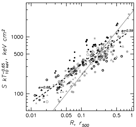
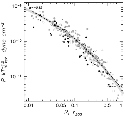
Figure 1: Comparison between the entropy and pressure of the sample and the non-parametric approximation used to study the dispersion. The entropy and pressure points corresponding to the same group are shown using the same symbol. The dashed line shows the results of the fit using the non-parametric locally weighted regression method. The dotted line in the entropy panel denotes the $S\sim r^{1.1}$ law, normalized to the results of Ponman et al. (2003). The grey line in the pressure panel shows the Sérsic model with n=4, which is remarkably close to the non-parametric fit.

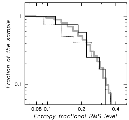
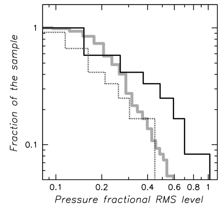
Figure 2: Cumulative distribution of groups vs fractional RMS scatter of the entropy (left panel) and pressure (right panel) parameter greater than the x-axis value. The black lines denote the results for our group sample, obtained using annuli and the mask sampling 2d variations in the temperature, marked as dotted and solid lines, respectively. The grey line represents the results of a 2d analysis performed on a sample of 208 modeled clusters (Finoguenov et al. in prep.). Our group sample exhibits a significantly larger scatter in the pressure, while the scatter in the entropy is comparable to simulations.

Table 6: Entropy and pressure fluctuations around the mean sample trend.

Name	$\sigma S$	$\sigma S$	$\sigma P$	$\sigma P$
	annuli	map	annuli	map
3C449	$0.25\pm 0.03$	$0.22\pm 0.02$	$0.03\pm 0.03$	$0.23\pm 0.04$
HCG 92	$0.11\pm 0.19$	$0.20\pm 0.14$	$0.42\pm 0.57$	$0.49\pm 0.21$
Pavo	$0.27\pm 0.10$	$0.19\pm 0.11$	$0.31\pm 0.12$	$0.50\pm 0.27$
HCG 42	$0.05\pm 0.12$	$0.28\pm 0.30$	$0.20\pm 0.47$	$0.63\pm 0.21$
HCG 68	$0.06\pm 0.04$	$0.22\pm 0.19$	$0.08\pm 0.21$	$0.32\pm 0.11$
NGC5171	$0.33\pm 0.09$	$0.42\pm 0.14$	$0.47\pm 0.05$	$0.22\pm 0.11$
HCG15	$0.08\pm 0.02$	$0.16\pm 0.04$	$0.10\pm 0.04$	$1.08\pm 0.09$
NGC507	$0.38\pm 0.13$	$0.08\pm 0.01$	$0.23\pm 0.19$	$0.08\pm 0.01$
NGC4073	$0.10\pm 0.09$	$0.10\pm 0.02$	$0.14\pm 0.13$	$0.12\pm 0.03$
NGC4325	$0.11\pm 0.10$	$0.33\pm 0.16$	$0.13\pm 0.10$	$0.42\pm 0.08$
NGC2563	$0.16\pm 0.17$	$0.16\pm 0.06$	$0.07\pm 0.08$	$0.15\pm 0.06$
NGC533	$0.22\pm 0.01$	$0.11\pm 0.01$	$0.12\pm 0.04$	$0.11\pm 0.03$
HCG 51	$0.20\pm 0.09$	$0.34\pm 0.19$	$0.28\pm 0.10$	$0.11\pm 0.15$
HCG 62	$0.18\pm 0.10$	$0.20\pm 0.03$	$0.11\pm 0.09$	$0.08\pm 0.02$

A remarkably high dispersion of points around the mean pressure trend is reported in Fig.2. A similar analysis has been carried out using a catalogue of 68 preheated clusters evolved with P3MSPH (Evrard 1988), with the details of the analysis presented in Finoguenov et al. (in prep.). The high dispersion in pressure could be formulated as a high fraction of the sample with rms exceeding a 30% value (42% vs 22% in the simulations) and also having 20% of the sample exhibiting a fractional rms exceeding 60%, when only 5% are expected. The Kolmogorov-Smirnov test returns the likelihood of the two samples being drawn from the same distribution of 1%. At the same time the likelihood that the rms in the entropy have a similar origin is 97%. A similar comparison for a representative cluster sample has been performed in Finoguenov et al. (2005b), where no deviations between the simulated and observed clusters were found, even though the data analysis technique was exactly the same as that used here, and the statistics of the observations were comparable to the current sample. Noting that the simulations used for comparison here were simulations of clusters, rather than groups, it appears that the excess dispersion seen in the pressure in Fig.2 is really a difference between groups and clusters, rather than one between simulations and observations. The good agreement seen in the entropy, disfavours any interpretation of the large scatter seen in groups in terms of differences in the thermodynamic history of the gas. We suggest that the differences really lie in the dark matter substructure, and should be further investigated in simulations. We note that in Mahdavi et al. (2005), a similar conclusion has been derived for some other groups individually, so we think that our result is representative.

This result is somewhat surprising, given that the CDM scenario predicts little dependence of the subhalo mass function on the mass of the host. A comparison with the data on the lowest mass scale, probed by observations of the nearby galaxies, reveals an opposite problem, as too few dwarf galaxies are found (e.g. Klypin et al. 1999). While a number of baryonic effects could be used to cure the problem on dwarf regime, these observations may shed light on the nature of the dark matter. Here we discuss a possible explanation within the framework of the conventional $\Lambda CDM$ model. In general, at an enhanced level of the entropy of the gas, typical of galaxy groups, one expects to diminish the effects of substructure (e.g. Kay et al. 2004), unless it retains its own gas. We stress once again, that difference in the average trend, also examined in Fig.2 using the annuli, can not account for the observed two-dimensional scatter. In our case, the most deviant points on the maps could often be associated with the location of major galaxies, yet the effect is not sufficient to disturb the entropy distribution. As at the moment we do not have simulations of groups to compare with, we postpone resolving this issue to the future work.

Another potentially important effect arises from the narrow redshift range of the groups in our sample. There is a known difference in the abundance of groups between the northern and southern hemispheres, associated with the presence of a large scale structure at $z\sim 0.02$ (Boehringer et al. 2002). Thus, further X-ray observations of a more distant group sample, such as available from the ROSAT 400 square degree survey (Burenin et al. 2006), are needed to study the influence of LSS on these conclusions.

3.1 Velocity structure of groups

Figure 3: Galaxy velocity histograms for the sample. The panels display the results obtained using the binning of the data of 200 km s^-1.

If, as suggested above, our group sample exhibits the presence of substructure in the dark matter, evidence of this might also be apparent in the velocity histograms of galaxies. To explore this, we collect them together in this section, although most of these histograms have been already published elsewhere (Zabludoff & Mulchaey 1998).

Fig.3 displays the velocity histograms of the sample, using a bin size of 200 km/s and including galaxies within the 1.2 Mpc of the group centre. A typical error on estimating the velocity is around 80–150 km/s. Evidence for substructure is present for 3C449, NGC5171, NGC507 and HCG15, although its exact quantification is difficult in most cases, due to the poor statistics. NGC4073, NGC2563, NGC533 and HCG62 appear to be regular groups. Some hints of substructure seen in the HCG62 histogram have been robustly identified through a refined method by Zabludoff and Mulchaey (1998). The available quality of the data is not sufficient for characterizing the degree of substructure to better than 20%, and a dedicated follow-up program is underway, the results of which will be reported elsewhere (Zimer et al. in prep.). With the currently available data, the conclusion is that, while in some cases (discussed in section 4 below) a detection of substructure provides supporting evidence of a link between the observed properties of the gas and the underlying dark matter distribution, it is not possible to derive quantitative conclusions without a much larger spectroscopic database on group members. Typically, a minimum of 100 group members with redshift measurements is required for such a study.

The brightest group member is always an elliptical, except for HCG92, where it is a lenticular. However, a complex galaxy (e.g. a double galaxy) in the centre is present for HCG 68, HCG 92, NGC 4073, Pavo, 3C449, HCG 51, NGC 507, HCG 62. Pavo, HCG51, NGC4073 contain more than one spiral galaxy.

4 Individual properties of the groups

We will follow a similar scheme when presenting the results for every system. As described in captions to Fig.LABEL:r:3c449, from top to bottom, left panels show the profiles of entropy, pressure, temperature and Fe abundance. The results obtained using annuli are shown in grey. The results from two-dimensional analysis (black crosses) are both shown as maps in the central panels and are converted into the profiles by plotting the observed values vs the distance of the extraction area from the centre. The dashed line in the entropy panel shows $S\propto r^{1.1}$, expected from simulations, normalized to the universal entropy scaling relation of Ponman et al. (2003). The non-parametric model for entropy and pressure are plotted as dashed line in the corresponding panels. Entropy and pressure maps are displayed as their ratios to the non-parametric model. From top to bottom, right panels show the results of image analysis: entropy, pressure, temperature maps, and surface brightness in the 0.5-2 keV band, where the temperature has been estimated through the hardness ratio of the 0.5–1 and 1–2 keV bands. Coordinates on the images are in units of $r_{500}$. The iron abundance is given in the photospheric solar units of Anders & Grevesse (1989).

Within the scenario of smoothness of accretion (e.g. Voit et al. 2003; Borgani et al. 2005), lumpy accretion should lead to lower entropy in group outskirts. At the same time, this would produce a large degree of variance in the central regions. While this is true for 3C449, a subsample of systems with lower entropy at outskirts, which includes 3C449, Pavo, NGC5171, NGC4073, NGC533, NGC4325 and HCG62, does not encompass all deviant systems. Some systems with high entropy at outskirts, such as HCG51, HCG42, have large degree of substructure. In addition, the flat temperature profile of HCG51 and HCG42 is a rather striking feature, possibly suggesting a major merger. Thus, while mergers seem to account for all systems of high dispersion, they either result in flat temperature profiles or in flat entropy profiles, probably depending on the mass ratio of the merger. The low entropy at outskirts of some of the groups may indicate an infall of the gas which corresponds to the early stage of a merger. We associate flat temperature profiles with the late stages of mergers.

4.1 3C449

As the number of figures is 176 in this paper, they are omited in astro-ph version, please follow the pointer in the astro-ph abstract. The surface brightness of 3C449 (UGC 12064) is elongated in the NE-SW direction on scales of $0.3r_{500}$ and in addition the NE sector has an enhancement in the form of a long tail or an arc, extending from the centre to the NE and turning north at $0.1r_{500}$. The spectral analysis reveals that the SW sector exhibits both higher pressure and lower entropy relative to the corresponding model describing the profiles of 3C449. The NE sector has lower entropy and higher metalicity. In the entropy plots, the system appears as quite deviant, exhibiting practically constant entropy level from $\sim 0.1r_{500}$ to $0.7r_{500}$. The temperature only drops at the very centre of the system. The central drop in the Fe abundance could be an artefact due to large temperature diversity in the centre (Buote 2000).

4.2 HCG15

The wavelet analysis of HCG15 reveals an abundance of structure on scales from point sources to $0.3r_{500}$. All of the substructure associated with the extended source is centered on the member galaxies of HCG15. On the larger scale, only the surface brightness map was obtained. The spectral analysis using annuli reveals a typical pressure profile. The entropy profile is approaching the scaling predictions at $0.2r_{500}$. On the scaled entropy and pressure profiles HCG15 reveals the component at $0.1r_{500}$ distance to the centre, associated with one of the galaxies. An asymmetry in the X-ray appearance of HCG15 is entirely due to the member galaxies, which also is responsible for the non-monotonic radial behavior of the entropy in the analysis using annuli. The iron abundance is typically below 0.1 solar, which is surprisingly low at locations associated with the galaxies. The available statistics of the data preclude a more detailed spectral investigation. The outmost rings do not have sufficient flux from the source to constrain the temperature and are not shown in the plots. The observed part of the group is in good agreement with the scaling, making the case of HCG15 different from that of HCG 68 and HCG 92.

4.3 NGC2563

The entropy map appears to be quite regular. Only seven regions are available for detailed spectroscopy. The gas properties are traced to $0.6r_{500}$. The temperature is 0.9 keV in the centre, rising to 1.6 keV by $0.1r_{500}$ and then dropping. The iron abundance is 0.6 times solar at the centre, dropping to 0.2 solar value at outskirts. The entropy is high at the centre, approaching the sample average trend at $0.3r_{500}$. Thus, the low X-ray luminosity of NGC2563 is associated with an inflated group core, while the bulk properties of its IGM are typical, which is also seen in the pressure plot. On the other hand, the feedback effects inside $0.3r_{500}$ are remarkable. The entropy shows a shelf between the 0.1 and 0.3 $r_{500}$ and at the same time, the inward raise in the pressure from $0.3r_{500}$ becomes immediately flatter, which for a similar mass profile is expected when gas becomes lighter. Such behavior of pressure supports the idea that the high entropy level is a dominating feature of the gas between 0.1 and 0.3 $r_{500}$. At very centre, however, the entropy of NGC2563 becomes typical.

4.4 HCG42

For the central elliptical the temperature is 0.75 keV and the iron abundance is 0.5 solar. The temperature slowly rises outwards reaching 0.85 keV. On the pressure map, the eastern part appears enhanced, indicating substructure. The eastward part of HCG 42 has lower entropy compared to the model, which is also associated with lower metalicity. On the entropy plot, HCG42 appears to approach the general behaviour for groups starting at $0.2r_{500}$, meaning that HCG42 should be considered as a virialized group, though affected by additional feedback effects. Apart from the substructure to the east, on the pressure plot HCG42 also appears as a normal group. We see no substantial deviations from Gaussianity in the the velocity histogram of HCG42.

4.5 NGC507

Within the central $0.2r_{500}$ NGC 507 exhibits an elongation in the surface brightness in the NW-SE direction, which is particularly outstanding in the NW, where a spectral analysis reveals lower entropy, higher pressure and higher metalicity. Two central galaxies are seen in NGC507, and the velocity histogram supports the idea of substructure. The temperature structure needs more than one component for the region centered on the galaxy. The temperature lies mostly in the 1.0–1.3 keV range, with iron abundance exceeding 0.5 solar, dropping to 0.35 in the outermost region. On large scales, the system is relaxed. The gas properties are traced out to $r_{500}$ and are consistent with standard entropy scaling. In the outskirts the pressure profile is very steep compared to average trends for the groups. A rise of both entropy and pressure to the scaling at the outmost point may not be representative for this system, since only a small part of the system is observed at this radius, as a result of the instrumental setup of the observation, in which the centre of NGC 507 was shifted to the corner. Higher entropy and lower pressure are usually found in simulations in the direction perpendicular to the alignment of filaments (Kravtsov, A. 2004, private communication).

4.6 HCG 68

HCG 68 is one of the most underluminous systems in the sample. HCG 68 reveals higher entropy to the east and north of the centre, as seen in both the hardness ratio based analysis and direct spectral fitting. The temperature behavior is nearly isothermal at the $\sim 0.64$ keV level. Hotter temperature zones are seen to the north, typically on the 0.75 keV level with a maximum of 0.9 keV. The entropy of HCG68 is traced to $0.3r_{500}$ where it is still higher than predictions from scaling. The deviations from the scaling are the largest for this system and are similar to HCG92: very high entropy and very low pressure of the gas. As appears to be the case for HCG92, major galaxy merger events within a low-mass group is a probable explanation for the presence of the X-ray emission. From the three galaxies located at the group’s center, at least two are spirals. On the other hand, the low metalicity of the gas restricts the contribution from stellar mass loss. If the origin of the hot gas is similar to HCG 92 – heating of the HI – the low metalicity should match the metalicity of the HI phase. The velocity histogram exhibits skewness, indicative of infall, while the mean temperature appears to be too hot compared to expectations for both the measured velocity dispersion and the normalization of the pressure profile.

4.7 Pavo

The central part of the group contains two major galaxies. The coordinate grid is centered on the elliptical and the spiral is located at (0.35,0.30) and is associated with an enhancement in the X-ray surface brightness. In X-rays, there is a bridge between the two major galaxies, with a possible sign of interaction on the side of the spiral. The temperature around the main elliptical is 0.9 keV and declines outward reaching the $\sim 0.5$ keV level. The spiral galaxy exhibits a low temperature of emission. Pavo groups exhibits a quite low level of entropy between $0.3-0.7r_{500}$ compared to the average trend. The pressure profile shows an enhancement at these radii, associated with the location of the spiral.

4.8 HCG 92

A detailed analysis of the XMM-Newton observations of the HCG 92 is presented in Trinchieri et al. (2005). A remarkable feature of HCG 92 consists in the shock heating of HI (Trinchieri et al. 2003). The X-ray surface brightness enhancement, which is extended in origin, as revealed by Chandra, is seen in Fig.LABEL:r:h92 as an extension from the centre to 0.1 towards the south in the surface brightness. The most surprising finding of our comparative analysis is that, despite a completely different origin for the X-ray gas, its entropy and pressure does not deviate from the mean trend for groups.

The average temperature of the IGM in HCG 92 is $\sim 0.6$ keV, with hotter regions located in the south-east. The element abundance profile rises with radius, indicating a lower metalicity for the recently heated gas. However, a downward bias in derived abundance due to complexity of the temperature structure (Buote 2000), is also possible. The entropy and pressure profiles are traced out to $0.3r_{500}$, where they start to deviate from the mean trend seen for groups. Such deviations could potentially be used to delineate the low-mass groups with high X-ray luminosity, caused by merger events.

At a distance of $0.3r_{500}$, there are zones of enhanced pressure and temperature, which have low metalicity. We associate these zones with the heating of the infalling low-metalicity material.

4.9 MKW4

The level of fluctuations in the entropy and pressure in IGM of MKW4 is rather moderate, indicating that the system is close to hydrostatic equilibrium. In the centre, the temperature is 1.6 keV and the iron abundance of 1.5 solar. The temperature initially rises to 2.2 keV, then declines. Iron abundance drops to the 0.2 solar level. Outside $0.1r_{500}$ the entropy of MKW4 is lower than predicted by the scaling. The largest deviations from spherical symmetry are seen in entropy $0.2r_{500}$ west from the centre and could be explained as the fossil record of a previous minor merger. The temperature profile presented here agrees with the Chandra results in Vikhlinin et al. (2005), the Chandra/XMM analysis of Fukazawa et al. (2004) and the ROSAT/ASCA results in Finoguenov et al. (2000). Deviant results are presented in O’Sullivan et al. (2003), based on a similar XMM dataset, but erroneously taking the MKW4 emission within the XMM FoV for the ’soft excess’ associated with foreground.

4.10 NGC5171

A detailed analysis of NGC5171 is presented in Osmond et al. (2004), where the appearance of the group has been explained by the merger of two groups, with a distant group appearing in projection in the south-east, which in our maps appears as the most deviating point in both the entropy and pressure maps. Entropy to the north is low, and represents the stripping tails of the interaction. Also, an elongation in the pressure to the north suggests that the dark matter potential of the infalling group has not been destroyed yet. The global properties of the system on large scales are quite normal, in both entropy and pressure, indicating that although the interaction has an effect on the luminosity of the object, it does not affect the bulk of the gas outside $0.3r_{500}$. The overall pressure level is low, which indicates that the temperature of the system used for scaling has been boosted by 20%. This corresponds to differences between the adopted temperature measured between 0.1 and $0.3r_{500}$, where in fact the interaction between the groups occurs, and the temperature measured between 0.3 and $0.7r_{500}$. The element abundance is low in most regions and is poorly constrained.

4.11 HCG62

Within $0.1r_{500}$, HCG62 exhibits an interesting bubble-like temperature structure and cool extensions to the north, which have also been reported in the Chandra observations (Vrtilek et al. 2002). On larger scales, the distribution of IGM properties is very symmetrical. Temperature is 0.8 keV at the centre rising to 1.3 keV before starting to fall back to 0.8 keV. On the entropy plot HCG62 exhibits a plateau between 0.1 and $0.3r_{500}$ with entropy lower than the scaling relation predicts, but then starts to rise again. We associate such behavior with the infall zone, also evident in the velocity histogram. HCG 62 provides an important example; the entropy profile is flat within a substantial part of the group and is at the level of 100 keV cm², yielding small values of beta in the surface brightness analysis, and yet it can hardly be the result of feedback, as the entropy of the gas is lower than seen on average. The overall level of the pressure is high in HCG62, probably due to an underestimate of the scaling temperature by 20% due to low entropy inclusions.

4.12 NGC4325

NGC4325 deviates strongly from the mean trend of the sample, e.g. the surface brightness profile for this group is very peaked, at odd with the generally flatter profiles of other systems. As a result, we obtain large dispersion values for it. Within the central $0.2r_{500}$ the entropy profile follows closely the expectation for cool core systems, and there is a corresponding pressure enhancement. These measurements reflect a very peaked surface brightness profile for this group, compared to other systems. Outside the central $0.2r_{500}$, the system regains a typical entropy and pressure level. The Fe abundance steadily declines with radius. The high metalicity ring at $0.4r_{500}$ distance from the centre is not very significant. The temperature behaviour is typical, consisting of initial raise from 0.8 keV, flattening at 1 keV and a subsequent decline reaching 0.6 keV at $r_{500}$.

4.13 NGC533

The IGM of NGC 533 shows typical profiles for both pressure and entropy. The gas is traced out to $0.7r_{500}$. The temperature raises from 0.9 at the centre to 1.4 and then falls to 0.8 keV at the limit of observation. The velocity histogram shows two peaks, the location of the two subgroups corresponding to the elongation in the surface brightness in the NE–SE direction. In the maps, a distinct difference between north-eastern and south-western parts of the group is seen. The north-east is hotter, mostly due to the high entropy, with surprisingly higher Fe abundance. We associate these features with incomplete mixing after the merger of the two groups, which is also responsible for the anisotropy in the velocity histogram of galaxies. The pressure plot indicates that the scaling temperature of the system has been boosted by 20%. This indicates that it is the NE part of the group that is affected by merging.

4.14 HCG51

The statistics of the XMM observations of HCG 51 are rather poor, as only 5 ksec was left after the flare cleaning. However, a number of interesting features are seen. On average, the temperature exhibits an isothermal behavior to $0.7r_{500}$, and a lack of metalicity gradient, confirming the results of the study of Finoguenov & Ponman (1999) and is suggesting a recent major merger. Hotter zones are seen to the south-west at $0.2r_{500}$ and to the west at $0.5r_{500}$. The iron abundance is also enhanced there. On small scales, the surface brightness reveals a number of asymmetries, which we were not able to resolve spectroscopically. The observed picture suggests incomplete mixing after a recent merger. HCG 51 is also a very dense system in the optical. On the entropy profile, the system reveals quite a high entropy level in its outskirts. The overall pressure level is low, suggesting that the scaling temperature has been boosted by 10%.

5 Summary

We have performed a detailed study of the IGM in a representative sample of groups of galaxies observed by XMM-Newton, which has been primarily drawn from the sample of Mulchaey et al. (2003). Comparing the entropy and pressure profiles of these groups with typical cluster profiles, scaled using the prescription of Ponman et al. (2003), we perform a non-parametric orthogonal regression analysis and obtain the typical entropy and pressure profile of the sample. In comparison to the commonly adopted $r^{1.1}$ behaviour for the entropy, the averaged profile for the groups is flatter, $r^{0.6-0.7}$, which is due to two effects: feedback in the group centres and the influence of infall in the outskirts. The averaged pressure profile has a slope of $-0.8$ within $0.1r_{500}$, and gradually steepens, reaching a slope of $-1.4$, which at the same radii is still shallower compared to the value of $-2.5$ reported in the similar analysis of clusters of galaxies (Finoguenov et al. 2005), and the overall mean pressure profile is well described by a Sérsic law with $n=4$.

The analysis using annuli may result in a somewhat steeper entropy profiles, compared to the results reported here. As discussed in Xu et al. (2004), a two-temperature model accounting for mixing of components with different entropy, assuming they are in the pressure equilibrium, also results in a flatter entropy profile. So, it might be that a two-dimensional modelling starts to resolve those components and reveals on average higher entropy at the center, just like the two-temperature approach. There are however, several pitfalls here. One is that we cannot verify this by performing a two-temperature fit, as the binning of the regions would suffer from high requirements on the statistics of the spectra imposed by a two temperature model. On the other hand an assumption of pressure equilibrium is not often justified, as shock wave driven by AGN are often observed as in e.g. M87 (Forman et al. 2005) and the Perseus cluster (Fabian et al. 2005).

An abundance of substructure has been identified in the sample, most of which we associate with the debris of recent mergers, usually seen as incomplete gas mixing. We also identify cases where the gas simply traces the dark matter substructure. In most cases we see also anisotropy in the velocity distribution of the galaxies, though our statistics are generally poor.

Our two-dimensional study yields high dispersion values for the pressure, compared to numerical simulations, which describe well the trends observed in clusters of galaxies. On the other hand, the scatter in the entropy is found to be as predicted in the simulations and is similar to that in clusters. This could either mean that the subhalo mass function in groups is different to that of the clusters, or that the substructure is better seen over the fainter mean trends typical of groups. We also mention that the sample selection correspond to a single large scale structure and studies covering larger redshift depth are required to firmly establish our findings.

We find that the state of the IGM resulting from galaxy merging, as observed in HCG 92, resembles closely the scaled properties of luminous galaxy groups. Thus, even using entropy and pressure it will be hard to identify the low-mass groups upscattered in their $M-L_{x}$ relation due to merger events, as discussed in Stanek et al. (2006).

6 Acknowledgments

The XMM-Newton project is an ESA Science Mission with instruments and contributions directly funded by ESA Member States and the USA (NASA). The XMM-Newton project is supported by the Bundesministerium fuer Wirtschaft und Technologie/Deutsches Zentrum fuer Luft- und Raumfahrt (BMWI/DLR, FKZ 50 OX 0001), the Max-Planck Society and the Heidenhain-Stiftung, and also by PPARC, CEA, CNES, and ASI. AF acknowledges support from BMBF/DLR under grant 50 OR 0207 and MPG. AF&MZ thank the Birmingham University for hospitality during their visits. The authors thank the referee for a careful reading of the manuscript and providing useful suggestions on presentation of the material.

References

- (1) Anders E., & Grevesse N., 1989, GeCoA, 53, 197
- (2) Böhringer, H., Collins, C. A., Guzzo, L., et al. 2002 ApJ, 566, 93
- (3) Borgani S., Governato F., Wadsley J., Menci N., Tozzi P., Lake G., Quinn T., Stadel J., 2001, ApJ, 559, L71
- (4) Borgani S., Finoguenov A., Kay S. T., Ponman T. J., Springel V., Tozzi P., & Voit G. M., 2005, MNRAS, 361, 233
- (5) Buote D. A., Canizares C. R., 1994, ApJ, 427, 86
- (6) Buote D. A., 2000, MNRAS, 311, 176
- Burenin et al. (2006) Burenin R. A., Vikhlinin A., Hornstrup A., Ebeling H., Quintana H., Mescheryakov A., 2006, ApJS subm., (arXiv:astro-ph/0610739)
- Evrard (1988) Evrard A. E., 1988, MNRAS, 235, 911
- Fabian et al. (2006) Fabian A. C., Sanders J. S., Taylor G. B., Allen S. W., Crawford C. S., Johnstone R. M., Iwasawa K., 2006, MNRAS, 366, 417
- Finoguenov & Ponman (1999) Finoguenov A., Ponman T. J., 1999, MNRAS, 305, 325
- Finoguenov, David, & Ponman (2000) Finoguenov A., David L. P., Ponman T. J., 2000, ApJ, 544, 188
- (12) Finoguenov A., Reiprich T., Böhringer H., 2001, A&A, 368, 749
- (13) Finoguenov A., Jones C., Böhringer H., & Ponman T. J., 2002, ApJ, 578, 74
- (14) Finoguenov A., Borgani S., Tornatore L., Böhringer H., 2003, A&A, 398, L35
- (15) Finoguenov A., Burkert A., Böhringer H., 2003b, ApJ, 594, 136
- (16) Finoguenov A., Pietsch W., Aschenbach B., Miniati F., 2004, A&A, 415, 415
- (17) Finoguenov A., Davis D. S., Zimer M., Mulchaey J. S., 2006, ApJ, 646, 143
- (18) Finoguenov A., Böhringer H., Zhang Y.-Y., 2005, A&A, 442, 827
- Finoguenov et al. (2005) Finoguenov A., Böhringer H., Osmond J. P. F., Ponman T. J., Sanderson A. J. R., Zhang Y.-Y., Zimer M., 2005b, AdSpR, 36, 622
- Forman et al. (2005) Forman W., et al., 2005, ApJ, 635, 894
- (21) Fukazawa Y., Kawano N., Kawashima K., 2004, ApJ, 606, L109
- (22) Garcia A. M., 1993, AAPS, 100, 47
- (23) Geller M. J., & Huchra J. P., 1983, ApJS, 52, 61
- (24) Henry J. P., Finoguenov A., & Briel U. G., 2004, ApJ, 615, 181
- (25) Huchra J. P., & Geller M. J., 1982, ApJ, 257, 423
- (26) Jansen F., Lumb D., Altieri B., et al., 2001, A&A, 365, L1
- (27) Kay S. T., Thomas P. A., Jenkins A., Pearce F. R., 2004, MNRAS, 355, 1091
- (28) Kravtsov A. V., Vikhlinin A., Nagai D., 2006, ApJ, subm., (arXiv:astro-ph/0603205)
- Klypin et al. (1999) Klypin A., Kravtsov A. V., Valenzuela O., Prada F., 1999, ApJ, 522, 82
- (30) Lisenfeld U., Braine J., Duc P.-A., Brinks E., Charmandaris V., Leon S., 2004, A&A, 426, 471
- Kravtsov, Vikhlinin, & Nagai (2006) Kravtsov A. V., Vikhlinin A., Nagai D., 2006, ApJ, 650, 128
- Mahdavi et al. (2000) Mahdavi A., Böhringer H., Geller M. J., Ramella M., 2000, ApJ, 534, 114
- (33) Mahdavi A., Finoguenov A., Böhringer H., Geller M. J., & Henry J. P., 2005, ApJ, 622, 187
- (34) Maia M. A. G., da Costa L. M., Latham D. W., 1989, ApJS, 69, 809
- (35) Majumdar S., Mohr J. J., 2004, ApJ, 613, 41
- (36) Mulchaey J. S., Davis D. S., Mushotzky R. F., Burstein D., 2003, ApJS, 145, 39
- (37) Nolthenius R., 1993, ApJS, 85, 1
- (38) Osmond J. P. F., Ponman T. J., 2004, MNRAS, 350, 1511
- (39) Osmond J. P. F., Ponman T. J., Finoguenov A., 2004, MNRAS, 355, 11
- (40) Osmond J. P. F., Ponman T. J., Finoguenov A., 2006, MNRAS, subm.
- (41) O’Sullivan E., Vrtilek J. M., Read A. M., David L. P., Ponman T. J., 2003, MNRAS, 346, 525
- (42) Ponman T. J., Cannon D. B., Navarro J. F., 1999, Nature, 397, 135
- (43) Ponman T. J., Sanderson A. J. R., Finoguenov A., 2003, MNRAS, 343, 331
- (44) Pratt G. W., Arnaud M., 2003, A&A, 408, 1
- (45) Pratt G. W., Arnaud M., 2005, A&A, 429, 791
- (46) Rasmussen J., et al. 2006, MNRAS, subm.
- (47) Read A. M., Ponman T. J., 2003, A&A, 409, 395
- (48) Reiprich T. H., Böhringer H., 2002, ApJ, 567, 716
- (49) Rossetti M., Ghizzardi S., Molendi S., Finoguenov A., 2005, A&A, in press, (astro-ph/0611056)
- (50) Sanderson A. J. R., Finoguenov A., Mohr J. J., 2005, ApJ, 630, 191
- (51) Sérsic, J.L. 1968, Atlas de Galaxies Australes (Coórdoba: obs. Astron., Univ. Nac. Córdoba)
- (52) Springel V., Hernquist L., 2003, MNRAS, 339, 289
- Stanek et al. (2006) Stanek R., Evrard A. E., Böhringer H., Schuecker P., Nord B., 2006, ApJ, 648, 956
- Streblyanska et al. (2006) Streblyanska A., Bergeron J., Brunner H., Finoguenov A., Hasinger G., Mainieri V., 2006, IAUS, 230, 450
- (55) Strüder L., Briel U.G., Dennerl K., et al., 2001, A&A, 365, L18
- (56) Sun M., Forman W., Vikhlinin A., Hornstrup A., Jones C., Murray S. S., 2003, ApJ, 598, 250
- (57) Tozzi P., & Norman C., 2001, ApJ, 546, 63
- (58) Trinchieri G., Sulentic J., Breitschwerdt D., Pietsch, W., 2003, A&A, 401, 173
- (59) Trinchieri G., Sulentic J., Pietsch W., Breitschwerdt D., 2005, A&A, 444, 697
- (60) Vikhlinin A., McNamara B. R., Forman W., Jones C., Quintana H., Hornstrup A., 1998, ApJ, 502, 558
- Vikhlinin et al. (2005) Vikhlinin A., Markevitch M., Murray S. S., Jones C., Forman W., Van Speybroeck L., 2005, ApJ, 628, 655
- (62) Voit G. M., Bryan G. L., 2001, Natur, 414, 425
- (63) Voit G. M., Balogh M. L., Bower R. G., Lacey C. G., Bryan G. L., 2003, ApJ, 593, 272
- (64) Voit G. M., Ponman, T. J., 2003, ApJL, 594, L75
- (65) Voit G. M., 2005, RvMP, 77, 207
- Vrtilek et al. (2002) Vrtilek J. M., Grego L., David L. P., Ponman T. J., Forman W., Jones C., Harris D. E., 2002, APS..APRB, 17107
- Xue, Böhringer, & Matsushita (2004) Xue Y.-J., Böhringer H., Matsushita K., 2004, A&A, 420, 833
- (68) Zabludoff A. I., Mulchaey J. S., 1998, ApJ, 496, 39
- (69) Zhang Y.-Y., Finoguenov A., Böhringer H., Ikebe Y., Matsushita K., Schuecker P., 2004, A&A, 413, 49