Mesoscale flows in large aspect ratio simulations of
turbulent compressible convection

We present the results of a very large aspect ratio ($A=42.6$) numerical simulation of fully compressible turbulent convection in a polytropic atmosphere, and focus on the properties of large-scale flows. Mesoscale patterns dominate the turbulent energy spectrum. We show that these structures, which had already been observed in Boussinesq simulations by Cattaneo et al. (2001), have a genuine convective origin and do not result directly from collective interactions of the smaller scales of the flow, even though their growth is strongly affected by nonlinear transfers. If this result is relevant to the solar photosphere, it suggests that the dominant convective mode below the Sun’s surface may be at mesoscales.

1 Introduction

The origin of solar photospheric flows on horizontal scales larger than granulation ($\ell\sim 1\leavevmode\nobreak\ 000$ km) has been a puzzling problem for more than forty years, when supergranulation ($\ell\sim 30\leavevmode\nobreak\ 000$ km) was discovered by Hart (1954) and later on confirmed by Simon & Leighton (1964). Even though recent breakthroughs in the field of supergranulation imaging have been made thanks to the emergence of local helioseismology techniques (Duvall & Gizon 2000) and the results of the MDI instrument (Hathaway et al. 2000), its origin is still unclear. The existence of an intermediate scale, mesogranulation ($\ell\sim 8\leavevmode\nobreak\ 000$ km), is also a matter of debate (Hathaway et al. 2000; Shine et al. 2000; Rieutord et al. 2000; Lawrence et al. 2001).

Meso and supergranulation have long been believed to be due to Helium deep recombinations driving cell-like convection. This view now appears to be out of date (Rast 2003). Several numerical experiments of convection (Cattaneo et al. 1991; Stein & Nordlund 2000) at moderate aspect ratio ($A$ is the ratio of the box width to its depth) have shown a tendency of long-lived large-scale flows to form in depth. Using large aspect ratio ($A=20$) simulations of Boussinesq convection, Cattaneo et al. (2001) have suggested that mesogranulation may result from nonlinear interactions of granules (see also Rast 2003). A large scale instability (Gama et al. 1994) of granules has also been proposed by Rieutord et al. (2000) to explain supergranulation. Local numerical simulations at $A=10$ (Rieutord et al. 2002) did not confirm it. DeRosa et al. (2002), using spherical simulations, have computed flows down to supergranular scales. Actually, the emergence of the three distinct scales of granulation, mesogranulation, and supergranulation in the surface layers, among the observed continuum of scales, remains a fully open problem that still deserves much work.

In this Letter, we report new results on three-dimensional numerical simulations of fully compressible turbulent convection in a rectangular box with very large aspect ratio $A=42.6$. This configuration allows us to study accurately the turbulent dynamics at horizontal scales between granulation and supergranulation, which have not been covered by previous numerical simulations. A compressible fluid is used to provide a more realistic model of photospheric convection than a Boussinesq fluid. Also, density stratification should attenuate the effect of an artificial bottom boundary (Nordlund et al. 1994).

In Sect. 2 we present our numerical setup and physical model. Section 3 is devoted to the analysis of the flow. The main consequences of the results are discussed in Sect. 4, which is followed by a short conclusion.

2 Numerical model and run parameters

For the purpose of our investigations we use a code designed to solve the fully compressible hydrodynamic equations for a perfect gas (e. g.  Cattaneo et al. 1991) in cartesian geometry. Constant dynamical viscosity and thermal conductivity are assumed. A constant thermal flux is imposed at the bottom, while temperature is held fixed at the surface. The velocity field satisfies stress-free impenetrable boundary conditions. The initial state is a $m=1$ polytropic atmosphere ($\gamma=5/3$) with small random velocity $\@vec{v}$, temperature $\theta$, and density $\rho$ perturbations. The initial density contrast between the bottom and top plates is 3, a value for which most of the features of stratification are already present in the linear convective instability problem (Gough et al. 1976). The Prandtl number is $\mathrm{Pr}=0.3$ and the Rayleigh number evaluated in the middle of the layer is $\mathrm{R}=3\leavevmode\nobreak\ 10^{5}$ (650 times supercritical). We do not paste several smaller boxes initially, as was the case in the paper by Cattaneo et al. (2001), thus there is no artificial spatial symmetry at $t=0$.

A sixth-order compact finite difference scheme (Lele 1992) is used in the vertical (gravity $\@vec{g}$) direction and a spectral scheme in the horizontal (periodic) directions. FFTs are implemented via the MPI version of FFTW (Frigo & Johnson 1998). Dealiasing by removal is performed using the 2/3 rule (Canuto et al. 1988). Time-stepping is done with a third-order, low-storage, fully explicit Runge-Kutta scheme. Energy dissipation is handled by laplacian terms, without any subgrid-scale modelling or hyperviscosity. A very large aspect ratio $A=42.6$ was achieved using $82\times 1024\times 1024$ grid points. The simulation ran on 64 processors and a total of 400 GB of raw data was collected throughout the numerical experiment.

3 Results

In the following, the depth of the layer $d$ is used as unit of length and the vertical thermal diffusion time $d^{2}/\kappa_{\mathrm{bot}}$ as unit of time ($\kappa_{\mathrm{bot}}$ is the thermal diffusivity at the bottom of the layer).

3.1 Flow structure and evolution

We first describe the flow evolution during 0.7 thermal diffusion time, corresponding to twelve turnover times (twice the vertical crossing time based on the r.m.s. velocity). Initially, linear growth is observed for a normalized horizontal wavenumber $k\sim 45$ (length $\ell\sim 1$) predicted by linear theory. The maximum of the depth-dependent momentum spectrum (hats denote two-dimensional horizontal Fourier transforms)

$$E(k,z)=\int_{\Omega_{\@vec{k}}}\left|\widehat{(\rho\@vec{v})}^{\phantom{*}}\!\!{}_{\@vec{k}}(z)\right|^{2}k\,\mbox{d}\Omega_{\@vec{k}}$$ (1)

then progressively shifts from $k\sim 45$ to $k\sim 5-8$ ($\ell\sim 5-8$) at the end of the simulation (Fig. 1). As can be seen on Fig. 2, the integral scale reaches $L_{\mathrm{int}}\sim 7$. Horizontal temperature maps at different times (Fig. 3) clearly show that the dominant scale of the flow increases during the simulation. This coherent pattern is best seen in the middle of the layer, but most of the in-depth dynamics are still clearly visible in the surface layers. In the upper layers, a second distinct smaller scale appears (bottom-right picture of Fig. 3). Its vertical extent (0.2 $d$) corresponds to the surface region of superadiabatic stratification, while the interior is almost isentropic. Referring to the Sun, we shall identify this thermal boundary layer scale with granulation, thus the larger internal scale is a mesoscale.

Next we shall try to explain the growth and saturation of the integral scale as well as the origin of the observed mesoscales.

Figure 1: Normalized momentum $E(k,z)$ and temperature $E_{\theta}(k,z)$ power spectra at $t=0.7$ and $z=0.99$ (the temperature spectrum has been shifted). The maximum around $k\sim 7$ corresponds to mesoscales. Also, a significant power excess in $E_{\theta}(k,z)$ is observed around $k\sim 40$ close to the surface, in comparison to the deeper layers. This feature is associated with granulation in this simulation.

Figure 2: Integral scale $L_{\mathrm{int}}(z)\!=\!\frac{\pi}{2}\int k^{-1}E(k,z)\,\mbox{d}k\,\left/\,\int E(k,z)\,\mbox{d}k\right.$ evolution at $z=0.87$. This scale represents the most energetic flow structures.

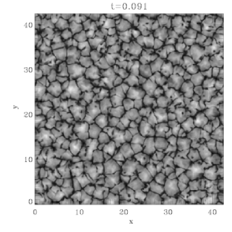
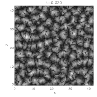
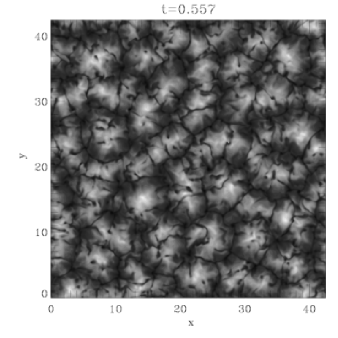
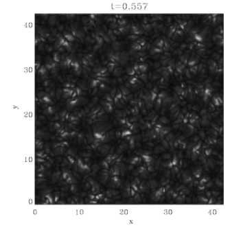
Figure 3: From left to right and top to bottom, time-evolution of temperature maps at $z=0.63$. The size of the visible mesoscale pattern increases until a quasi-steady state is reached (bottom-left image). Bottom-right picture: same as bottom-left image, for a surface layer ($z=0.99$), showing the differences between in-depth mesoscale dynamics and the smaller-scale flow in the upper thermal boundary layer.

3.2 Convective origin of mesoscales

After the linear growth, saturation of the velocity amplitude at $k\sim 45$ occurs. At that time, this mode is the scale of energy injection. Larger scales are also highly linearly unstable for $\mathrm{R}=3\leavevmode\nobreak\ 10^{5}$ and we observe that they continue to grow. However, in the nonlinear regime, energy transfer to smaller scales limits this growth. To show this, we take the horizontal Fourier transform of the momentum equation and extract its solenoidal part by applying the projection operator $\displaystyle{\mathcal{P}\left[\@vec{v}\right]\,=\,\@vec{v}-\@vec{\nabla}\!\Delta^{-1}\@vec{\nabla}\!\cdot\!{\@vec{v}}\,=\,\@vec{v}^{s}}$, denoted by $\mathcal{\widehat{P}}$ when acting on horizontally Fourier-transformed fields. Taking the dot product with the complex conjugate of the solenoidal part of momentum $\widehat{(\rho\@vec{v})^{s}}^{*}\!\!\!{}_{\@vec{k}}(z)$, integrating over depth $z$ and angles $\Omega_{\@vec{k}}$ in the horizontal spectral plane, we obtain a time-evolution equation for the solenoidal part $E^{s}(k,z)$ of $E(k,z)$, integrated vertically:

$$\partial_{t}\int_{0}^{1}\!\!\!E^{s}(k,z)\,\mbox{d}z=T(k)+F(k)+D(k),$$ (2)

$$T(k)=\displaystyle{-2\,\mathrm{Re}\left[\int_{0}^{1}\!\!\!\int_{\Omega_{\@vec{k}}}\!\!\!\widehat{(\rho\@vec{v})^{s}}^{*}\!\!\!{}_{\@vec{k}}\cdot\widehat{\mathcal{P}}\left[\widehat{\@vec{\nabla}\!\cdot\!{\left(\rho\@vec{v}\@vec{v}\right)}}_{\@vec{k}}\right]k\,\mbox{d}\Omega_{\@vec{k}}\,\mbox{d}z\right]},$$ (3)

$$F(k)=\displaystyle{2\,\mathrm{Re}\left[\int_{0}^{1}\!\!\!\int_{\Omega_{\@vec{k}}}\!\!\!\widehat{(\rho\@vec{v})^{s}}^{*}\!\!\!{}_{\@vec{k}}\cdot\widehat{\mathcal{P}}\left[\widehat{\rho\@vec{g}}_{\@vec{k}}\right]k\,\mbox{d}\Omega_{\@vec{k}}\,\mbox{d}z\right]}.$$ (4)

$T(k)$ represents nonlinear transfers, $F(k)$ is the forcing by buoyancy and $D(k)$, which has a similar definition, represents viscous dissipation. In Fig. 4, we plot these quantities averaged over a time interval during which $k>12$ modes are steady, while modes with smaller $k$ develop.

Figure 4: Depth-integrated spectral transfer $T(k)$, buoyancy forcing $F(k)$, dissipation $D(k)$ and net power injected in $\int E^{s}(k,z)\,\mbox{d}z$ following Eq. (2). An average between $t=0.14$ and $t=0.20$ has been taken to outline the mean growth of $k<12$ modes during this period owing to $F(k)$ (note especially that $T(k)<0$ for these scales). The maximum over $k$ of the depth-integrated spectrum has been used for normalizing.

We observe that $F(k)$ is the basic energy supply on large scales, as in the linear convective instability mechanism. Nonlinear transfer $T(k)$ is always negative for modes with $7\leq k\leq 11$, which have a small but positive net energy growth. Therefore large scales do not come out of nonlinear interactions but have a convective origin. This effect could also be observed using the energy equation: as in linear convection, energy is injected in large scales via the advection of the horizontally averaged entropy profile, while nonlinear transfers and diffusion only remove energy from them.

Note finally that the mesoscale pattern of Fig. 3 is expected to expand slightly on a much longer time scale that can not be achieved numerically. Also, the dominant scales may depend on the Rayleigh number, as they result from a balance between buoyancy and nonlinear transfers. These mesocells are very probably the same as those observed by Cattaneo et al. (2001) in Boussinesq simulations with $A=20$. Their size is comparable in both experiments. We therefore confirm these results for a compressible fluid, in a larger aspect ratio box with no initial symmetry, but interpret them quite differently.

4 Discussion

4.1 Relations with solar photospheric convection

We now discuss the relevance of our results to the Sun. First, an estimate of the size (in km) of the typical structures of our simulation can be computed to clarify the comparison with observations. Identifying the thermal boundary layer thickness with the typical vertical extent of solar granulation ($\sim 150$ km), we find our mesocells to be 6 000 km wide.

This numerical experiment represents a highly idealized model of photospheric convection, even though it integrates density stratification. Differences with observations or with more realistic simulations (Stein & Nordlund 1998) are therefore clearly expected. The most important one is the prominent peak at mesoscales in our power spectrum (Fig. 1), which might be due to boundary condition effects or to the absence of radiative transfer in our simulations. As noted by Cattaneo et al. (2001), granulation is directly related to the formation of a thermal boundary layer, so that changes in boundary conditions might have a strong impact on the contrast between mesogranular and granular flows. Also, in radiative convection simulations by Stein & Nordlund (2000) with an open bottom boundary, the dominant scale visually increases continuously with depth, which does not happen in our experiment. Besides, the absence of radiative transfer in our simulations makes it impossible to define a $\tau=1$ surface. Actually, the intensity map presented by Rieutord et al. (2002) does not exhibit clear mesoscale intensity modulation whereas temperature maps at fixed depth do. Since the $\tau=1$ surface does not correspond to a fixed depth, mesoscale convective flows may be present in the subsurface layers and be partly hidden this way.

Besides, various observations suggest some mesoscale organization. Oda (1984) has reported some clustering of granules around brighter granules distributed on mesoscales. In our simulation (Fig. 3), the imprint of mesoscales is very clear at the surface and clustering of smaller granules also occurs around bright spots corresponding to mesoscale upflows. Finally, a distribution of inter-network magnetic fields at the scale of mesogranulation has been found recently (Domínguez Cerdeña 2003; Roudier & Muller 2004), which might also be related to strong convective mesoscale plumes.

4.2 Very large scales

A final word must be said about very large-scale flows. According to the previous estimates, the horizontal size of our box is 35 000 km, which does not leave much room for supergranules. We do not obtain a second peak at small $k$ in the spectra, so there is strictly speaking no supergranulation in our simulation. This may be because we do not have the necessary physical ingredients in the model, because our box is not large or deep enough, or because our run is too short. However, noticeable positive nonlinear transfer occurs at the smallest $k$ (Fig. 4) and we observed weak horizontally divergent large-scale flows of still unclear origin. When subjected to horizontal strains, strong mesoscale vertical vortices resulting from angular momentum conservation in sinking plumes (Toomre et al. 1990) might help creating horizontal vorticity on large scales.

5 Conclusions

The results of our simulations of large-scale convection in a compressible polytropic atmosphere show that the dominant convective mode is found at mesoscales. We observe that large aspect ratio simulations are necessary to study the convective dynamics of these structures, since the integral scale is $L_{\mathrm{int}}\sim 7$ in the final quasi-steady state. A slow evolution is expected on longer time scales, which are unfortunately numerically out of reach. Some similarities with solar observations are found. If this kind of model is relevant to study the solar photosphere, our results suggest that mesoscale convection may be powerful below the Sun’s surface. This would help to explain the coexistence of two apparently distinct granular and mesogranular scales. Supergranulation is not found in this experiment.