UNIVERSE DRIVEN BY THE VACUUM OF SCALAR FIELD: VFD MODEL.

Abstract

It is shown that in the Vacuum Fluctuations Domination model (VFD), where vacuum fluctuations of scalar fields dominates under matter and radiation throughout the all history of the Universe expansion (gr-qc/0604020, gr-qc/0610148), acceleration parameter evolves monotonically from the zero to the present day negative value. That is according to this model the Universe has no decelerating past and conventional radiation domination and matter domination epochs are absent. Predictions of accelerating parameter for $z\sim 0-2$ is compared with that follows from the SN type Ia data.

Fast progress in accumulating and handling of the astrophysical data about the Universe expansion [1, 2, 3, 4, 5, 6] clears the way to testing of different models of the Universe evolution. Although, the $\Lambda\mbox{CMD}$ model is able to explain the observational data [7], it is necessary to provide a deeper insight into the cosmological constant problem [8, 9, 10, 11, 12, 13, 14, 15]. Among numerous approaches to the cosmological constant problem, the quantum field theory (QFT) approach may suggest some solutions.

It is well known that the covariant removing of all divergent terms from the energy-momentum tensor by some regularization procedure leads to the vacuum energy density $\rho_{vac}\sim 1/L^{4}$, where $L$ is the radius of the Universe curvature [16]. This quantity is too small to explain the observed Universe acceleration if one may identify $L$ with the size of a present day Universe.

On the other hand, the direct ultraviolet momentum (UV) cut-off for evaluation of the vacuum energy provides the enormous quantity $\rho_{vac}\sim M_{p}^{4}$, where $M_{p}$ is the Planck mass.

In our previous works [18, 19], the accelerated expansion of Universe was attributed to the back-reaction of vacuum fluctuations of massless scalar fields. It was found, that the use of UV cut-off at the Planck level in the equation of motion for the Universe scale factor instead of that in the Friedman equation allows explaining the observable value of Universe acceleration. In our approach, the effective density of dark energy is proportional to the Hubble constant squared $\rho_{vac}\sim H^{2}\kappa_{max}^{2}\sim H^{2}M_{p}^{2}$, as it occurs in the holographic dark energy models [20, 21, 22, 23, 24, 25] (here $\kappa_{max}$ denotes the UV cut-off of the present day physical momentums).

Below our previous model is summarized and compared with the SN Ia data and gamma ray busts data.

Let us write down the system of Friedman– Lemaître equations for the Universe scale factor $a$, the density of a matter $\rho$ and the pressure $p$:

$$-\frac{1}{2}M_{p}^{2}\left(a^{\prime 2}+{\mathcal{K}}a^{2}\right)+\rho a^{4}+\frac{1}{6}M_{p}^{2}\Lambda a^{4}=0,$$

$$M_{p}^{2}a^{\prime\prime}=-M_{p}^{2}\mathcal{K}a+(\rho-3p)a^{3}+\frac{2}{3}M_{p}^{2}a^{3}\Lambda,$$

$$\rho^{\prime}+3\frac{a^{\prime}}{a}(\rho+p)=0,$$ (1)

where the conformal time $\eta$ implying the metric $ds^{2}=a^{2}(\eta)(d\eta^{2}+d\sigma^{2})$ is used (the reason will be explained below), $\Lambda$ is the cosmological constant, $\mathcal{K}$ is the signature of space-time and the Planck mass $M_{p}$ should be read as $M_{p}=\sqrt{\frac{3}{4\pi G}}$.

The $\Lambda\mbox{CDM}$ model can be obtained by setting $p=0$, $\mathcal{K}=0$ and finally is reduced to the single equation

$$a^{\prime\prime}=2\frac{a^{\prime 2}}{a}-\frac{3}{2}a_{0}\mathcal{H}^{2}\Omega_{m},$$ (2)

where $a_{0}=a(0)$ is the present day scale factor (this moment corresponds to $\eta=0$ everywhere below), $\mathcal{H}=\frac{a^{\prime}}{a}\bigr{|}_{\small\eta=0}$ is the conformal Hubble constant and the constant $\Omega_{m}$ is connected with the matter density $\frac{1}{2}\Omega_{m}M_{p}^{2}\,\mathcal{H}^{2}a_{0}=\rho\,a^{3}=\rho_{0}a_{0}^{3}$.

Coming to the VFD model [18, 19] we set $\Lambda=0$, $p=0$, $\mathcal{K}=0$ and add a massless scalar field, which is characterized by the averaged pressure and the density:

$$\rho_{\phi}=\frac{1}{V}\int_{V}\left(\frac{\phi^{\prime 2}}{2a^{2}}+\frac{(\bm{\nabla}\phi)^{2}}{2a^{2}}\right)d^{3}\bm{r},$$

$$p_{\phi}=\frac{1}{V}\int_{V}\left(\frac{\phi^{\prime 2}}{2a^{2}}-\frac{(\bm{\nabla}\phi)^{2}}{6a^{2}}\right)d^{3}\bm{r},$$ (3)

where $V$ is some volume, which will be set to unity hereafter. The second step is to turn to the quasiclassical picture, where the scalar field $\hat{\phi}(\eta,\bm{r})$ is quantum. The resulting master equations for the VFD model are

$$-M_{p}^{2}\frac{a^{\prime 2}}{2}+\rho a^{4}+\int\left(\frac{a^{2}<0|{\hat{\phi}}^{\prime 2}|0>}{2}+\frac{a^{2}<0|(\bm{\nabla}{\hat{\phi}})^{2}|0>}{2}\right)d^{3}\bm{r}=const,$$

$$M_{p}^{2}a^{\prime\prime}=\rho a^{3}-\int\left(a<0|{\hat{\phi}}^{\prime 2}|0>-a<0|(\bm{\nabla}{\hat{\phi}})^{2}|0>\right)d^{3}\bm{r},~{}$$ (4)

$$\hat{\phi}^{\prime\prime}+2\frac{a^{\prime}}{a}\hat{\phi}^{\prime}-\Delta\hat{\phi}=0,~{}$$

where $<0|...|0>$ denotes a mean value over the vacuum state of scalar field. The first equation is the integral of motion for two last equations. However, it should be noted that it is not the Friedman equation because the constant on the right hand side is not zero. The point is that some renormalization is needed to avoid the cosmological constant problem, i.e. the huge QFT vacuum energy in the Friedman equation. Instead of determining the renormalization constant, one can consider two last equation and fix the constant assigning the initial condition for the equations. It is very important, that in conformal time a renormalization is not required for the second equation. The reason is that the equation contains exact difference of the kinetic and potential energies of the field oscillations. In the Minkowski space-time this difference is exactly zero by virtue of the virial theorem for an oscillator, which states that the kinetic energy is equal to the potential one in the virial equilibrium. In the expanding Universe this difference is proportional to the Hubble constant squared.

Scalar field can be decomposed in a complete set of the modes $\phi(\bm{r})=\sum_{\bm{k}}\phi_{\bm{k}}e^{i{\bm{k}}\bm{r}}$ and quantization of the modes consists in postulating [16]

$$\hat{\phi}_{\bm{k}}=\hat{\mbox{a}}^{+}_{-\bm{k}}\chi_{k}^{*}(\eta)+\hat{\mbox{a}}_{\bm{k}}\chi_{k}(\eta),$$ (5)

where complex functions $\chi_{k}(\eta)$ satisfy the relations:

$$\chi^{\prime\prime}_{k}+k^{2}\chi_{k}+2\frac{a^{\prime}}{a}{\chi^{\prime}}_{k}=0,$$

$$a^{2}(\eta)(\chi_{k}\,{\chi_{k}^{\prime}}^{*}-\chi_{k}^{*}\,\chi_{k}^{\prime})=i.$$ (6)

The adiabatic approximation

$$\chi_{k}(\eta)=\frac{\exp\left({-i\int_{0}^{\eta}\sqrt{k^{2}-\frac{a^{\prime\prime}(\tau)}{a(\tau)}}\,d\tau}\right)}{\sqrt{2}a(\eta)\sqrt[4]{k^{2}-\frac{a^{\prime\prime}(\eta)}{a(\eta)}}}$$ (7)

allows calculating the difference of the kinetic and potential energies of field oscillators up to the second-order terms:

$$\int\left(a<0|{\hat{\phi}}^{\prime 2}|0>-a<0|(\bm{\nabla}{\hat{\phi}})^{2}|0>\right)d^{3}\bm{r}=~{}~{}~{}~{}~{}~{}~{}~{}~{}~{}~{}~{}~{}~{}~{}~{}~{}~{}~{}~{}~{}~{}~{}~{}~{}~{}~{}~{}~{}~{}~{}~{}~{}~{}~{}~{}~{}~{}$$

$$\sum_{\bm{k}}a<0|\hat{\phi}^{\prime}_{\bm{k}}\hat{\phi}^{\prime}_{-{\bm{k}}}|0>-k^{2}a<0|\hat{\phi}_{\bm{k}}\hat{\phi}_{-{\bm{k}}}|0>=\sum_{\bm{k}}a({\chi_{k}^{\prime}}^{*}\chi_{k}^{\prime}-k^{2}\chi_{k}^{*}\chi_{k})\approx$$

$$\frac{1}{2}\left(-\frac{a^{\prime\prime}}{a^{2}}+\frac{{a^{\prime}}^{2}}{a^{3}}\right)\sum_{\bm{k}}\frac{1}{k}+O({a^{\prime}}^{3})+O(a^{\prime}a^{\prime\prime})+O(a^{\prime\prime\prime}),~{}~{}~{}~{}~{}~{}$$ (8)

where we imply that $a^{\prime}$ is the first-order quantity, $a^{\prime\prime}$ is the second-order one, $a^{\prime\prime\prime}$ is the third-order one and so on.

Using (8) in (4) leads to the master equation of VFD model in the form:

$$M_{p}^{2}a^{\prime\prime}=\frac{1}{2}\Omega_{m}M_{p}^{2}\mathcal{H}^{2}a_{0}+\frac{1}{2}\left(\frac{a^{\prime\prime}}{a^{2}}-\frac{{a^{\prime}}^{2}}{a^{3}}\right)\sum_{\bm{k}}\frac{1}{k}.$$ (9)

Eq. (9) can be integrated up to the equation

$$a^{\prime^{2}}=a_{0}^{2}\mathcal{H}^{2}{\frac{S_{0}-1-\Omega_{m}\left(a/a_{0}-1\right)}{S_{0}a_{0}^{2}/a^{2}-1}},$$ (10)

where the parameter $S_{0}$, from the one hand, is determined by the UV cut-off $\kappa_{max}$ of the physical momentums $\kappa=k/a_{0}$

$$S_{0}=\frac{1}{2M_{p}^{2}a_{0}^{2}}\sum_{\bm{k}}\frac{1}{k}=\frac{1}{M_{p}^{2}a_{0}^{2}(2\pi)^{3}}\int\frac{d^{3}\bm{k}}{2k}=\frac{\kappa_{max}^{2}}{8\pi^{2}M_{p}^{2}}$$

and, from the other hand, is connected with the present day deceleration parameter $q_{0}$ as $S_{0}=\frac{2q_{0}-2+\Omega_{m}}{2q_{0}}$. It was shown [18, 19] that the ultraviolet (UV) cut-off of the present day physical momentums $k/a_{0}$ in the sum $\sum_{\bm{k}}\frac{1}{k}$ at the Planck level $\kappa_{max}=k_{max}/a_{0}\sim M_{p}$ can explain the observed value of Universe acceleration. In principle, the exact value of UV cut-off has to result from the Planck scale physics.

A validity range of Eqs. (9), (10) is defined by the next terms in the expansion (8). According to Refs. [18, 19], the next terms contain additional multiplier $a^{\prime}/(ak_{max})$ as compared with the main term, where $k_{max}$ is the UV cut-off $k_{max}/a_{0}\sim M_{p}$ [18, 19]. Thus Eqs. (9), (10) are valid if $\frac{a^{\prime}}{a}\ll M_{p}a_{0}$, or $\dot{a}\ll M_{p}a_{0}$.

Eq. (10) can also be rewritten in a cosmic time $dt=a\,d\eta$

$$H^{2}=\left(\frac{\dot{a}}{a}\right)^{2}=H_{0}^{2}\frac{(S_{0}+\Omega_{m}-1)a_{0}^{4}a^{-4}-\Omega_{m}a_{0}^{3}a^{-3}}{S_{0}a_{0}^{2}a^{-2}-1},$$ (11)

which gives $a(t)\approx a_{0}H_{0}\sqrt{\frac{S_{0}+\Omega_{m}-1}{S_{0}}}\,t$ in the vicinity of $t=0$ (i.e. in the conformal time $a(\eta)=\mathcal{H}\sqrt{\frac{S_{0}+\Omega_{m}-1}{S_{0}}}\exp\left(\mathcal{H}\sqrt{\frac{S_{0}+\Omega_{m}-1}{S_{0}}}\,\eta\right)$). During the further evolution deceleration parameter

$$q(z)=-\frac{\ddot{a}a}{\dot{a}^{2}}=\frac{1+z}{H}\,\frac{dH(z)}{dz}-1=~{}~{}~{}~{}~{}~{}~{}~{}~{}~{}~{}~{}~{}~{}~{}~{}~{}~{}~{}~{}~{}~{}~{}~{}~{}~{}~{}~{}~{}~{}~{}~{}~{}~{}~{}~{}$$

$$\frac{q_{0}\left(\Omega_{m}(2q_{0}+\Omega_{m}-2)z^{2}+2\left(\Omega_{m}^{2}-3\Omega_{m}+2\right)z+(\Omega_{m}-2)^{2}\right)}{(\Omega_{m}+z(z+2)(2q_{0}+\Omega_{m}-2)-2)(\Omega_{m}+z(2q_{0}\Omega_{m}+\Omega_{m}-2)-2)},$$ (12)

comes from zero to the present day negative value at small red shifts $z=a_{0}/a-1$ as it is shown in Figs. 1,2.

The parameter $\Omega_{m}$ amounts 0.27 for both models and $q_{0}=-0.8$ for the VFD model. These values are chosen to fit the curves within a thin waist of the experimental data channel near z=0.2.

It is interesting that VFD model is highly insensitive to the dark matter content. We see that two curves corresponding to the $\Omega_{m}=0.27$ and $\Omega_{m}=0.04$ (pure baryonic matter!) almost coincide.

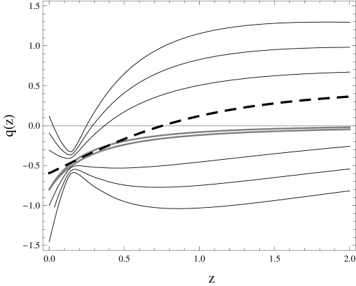
Figure 1: VFD curves (bold grey, $\Omega_{m}=0.27$ and $\Omega_{m}$=0.04) of the acceleration parameter evolution and that of $\Lambda{CDM}$ (dashed) put on the $1\sigma$, $2\sigma$, $3\sigma$ error channels (thin lines) of the reconstruction of the deceleration parameter [26] from the 115 SN Ia data.

It should be noted that in the case of $S_{0}=0$ our model turns formally into conventional model of the flat Universe filled with a dust and a relativistic matter. However, “matter domination epoch” and “radiation domination epoch” are in the non physical region after Big Rip, where the Hubble constant becomes infinite at some finite $a$ and $t$, when denominator in Eq. (11) tends to zero.

To summarize, we have considered the VFD model offered in our previous works [18, 19]. In this model, the Universe acceleration results from the vacuum fluctuations of fundamental scalar fields.

Main feature of the VFD model that it does not predict the change from a deceleration to an acceleration in the past. If the father observations will insist on such a change, some modification of VFD should be required, because it has no tuning parameters. Some possibility of such a modification is a theory based on the truncation of physical momentums $k/a(\eta)\sim M_{p}$ rather than that of static momentums $k\sim a_{0}M_{p}$. This would require a consideration in a system of reference, in which Universe looks like the Hoyle-Narlikar one [27, 28].

Another feature of the VFD model is that in principle the dark matter is not needed.

The authors are grateful to Yungui Gong and Anzhong Wang for kindly presented the deceleration parameter reconstruction data.

References

[1] S. Perlmutter et al.,
Astrophys. J.517, 565 (1999).
[2] P.M. Garnavich
et al., Astrophys. J.493, L53 (1998).
[3] A.G. Riess et al., Astron. J.116, 1009 (1998).
[4] C.L. Bennett et al., Astrophys. J. Supp. Ser.148, 1 (2003).
[5] D.J. Eisenstein et al., Astrophys. J.633, 560 (2005).
[6] A. G. Riess et al, astro-ph/0611572.
[7] V. Sahni and A. Starobinsky,
astro-ph/0610026.
[8] S. Weinberg, Review of Modern Physics61, 1 (1989).
[9] S.M. Carroll, Living Rev. Relativity4, 1 (2001).
[10] T. Padmanabhan, Phys. Rep.380, 235 (2003).
[11] J. R. Ellis, Phil. Trans. Roy. Soc. Lon. A361, 2607 (2003).
[12] P. J. Steinhard, Phil. Trans. Roy. Soc. Lon. A361, 2497 (2003).
[13] C. Armendariz-Picon, V. Mukhanov and P. J. Steinhardt, Phys. Rev. D63, 103510 (2001).
[14] Copeland E J, Sami M and Tsujikawa S,
hep-th/0603057.
[15] S. Räsänen, astro-ph/0607626.
[16] N.D. Birrell and P.C.W. Davis, Quantum Fields in Curved
Space
(Cambridge Univ. Press, 1982).
[17]
V. K. Onemli, R. P. Woodard, Phys.Rev. D70, 107301 (2004).
[18] S.L. Cherkas and V.L. Kalashnikov,
gr-qc/0604020.
[19] S.L. Cherkas and V.L. Kalashnikov, JCAP0701,
028 (2007),
gr-qc/0610148.
[20] A. G. Cohen, D. B. Kaplan and A. E. Nelson,
Phys.Rev.Lett.82, 4971 (1999).
[21] M. Li, Phys.Lett. B603, 1 (2004).
[22] R. Brustein and A. Yarom, JHEP0501,
046 (2005).
[23] T. Padmanabhan, Class.Quant.Grav.22,
L107 (2005).
[24] E. Elizalde, S. Nojiri, S.D. Odintsov and P. Wang, Phys.Rev. D71, 103504 (2005).
[25] A.E. Shalyt-Margolin, hep-th/0605236.
[26] Y. Gong and A. Wang, Phys.Rev. D73,
083506 (2006), astro-ph/0601453; astro-ph/0612196.
[27] F. Hoyle and J. V Narlikar, Proc. Roy. Soc. A282,
191 (1964).
[28] J. V. Narlikar and A. K. Kembhavi, Non-Standard
Cosmologies. in: The fundamentals of Cosmic Physics (Gordon and
Bridge, 1980).