The Co-Formation of Spheroids and Quasars Traced in their Clustering

Abstract

We compare observed clustering of quasars and galaxies as a function of redshift, mass, luminosity, and color/morphology, to constrain models of quasar fueling and the co-evolution of spheroids and supermassive black holes (BHs). High redshift quasars are shown to be drawn from the progenitors of local early-type galaxies, with the characteristic quasar luminosity $L_{\ast}$ at a given redshift reflecting a characteristic mass of the “active” BH/host population at that epoch. In detail, the empirically calculated clustering of quasar “remnants” (knowing the observed clustering of the original quasars) as a function of stellar mass and/or luminosity is identical to that observed for early-type populations. However, at a given redshift, the active quasars cluster as an “intermediate” population, reflecting neither “typical” late nor early-type galaxies at that redshift. Comparing with the age of elliptical stellar populations as a function of mass reveals that this “intermediate” population represents those ellipticals undergoing (or terminating) their final significant star formation activity at the given epoch. Assuming that quasar triggering is associated with the formation/termination epoch of ellipticals predicts quasar clustering at all observed redshifts without any model dependence or assumptions about quasar light curves, lifetimes, or accretion rates. This is not true for spiral/disk populations or the quasar halos (by any definition of their ages); i.e. quasars do not generically trace star formation or halo assembly/growth processes. Interestingly, however, quasar clustering at all redshifts is consistent with a constant host halo mass $\sim 4\times 10^{12}\,h^{-1}\,M_{\sun}$, similar to the local “group scale.” The observations support scenarios in which major mergers dominate the bright, high-redshift quasar population. We demonstrate that future observation of quasar clustering as a function of luminosity can be used to constrain different fueling mechanisms which may dominate AGN populations at lower luminosity and/or redshift. We also show that clustering measurements at $z=3-6$ will be sensitive to the efficiency of feedback or “quenching” at these redshifts.

1. Introduction

In recent years, it has become clear that essentially all galaxies harbor supermassive black holes (BHs) (e.g., Kormendy & Richstone, 1995), the masses of which are correlated with many properties of their host spheroids, including luminosity, mass (Magorrian et al., 1998), velocity dispersion (Ferrarese & Merritt, 2000; Gebhardt et al., 2000), concentration and Sersic index (Graham et al., 2001). Further, comparison of the relic BH mass density and quasar luminosity functions (QLFs; Soltan, 1982; Salucci et al., 1999; Yu & Tremaine, 2002; Marconi et al., 2004; Shankar et al., 2004; Hopkins et al., 2007b), the cosmic X-ray background (Elvis et al., 2002; Ueda et al., 2003; Cao, 2005; Hopkins et al., 2007b), and relic BH Eddington ratios (Hopkins, Hernquist, & Narayan, 2005) demonstrates that the growth of BHs is dominated by a short-lived phase of high accretion rate, bright quasar activity. This, together with the similarity between the cosmic star formation history (e.g., Hopkins & Beacom, 2006) and quasar accretion history (e.g., Merloni et al., 2004; Hopkins et al., 2007b), reveals that quasar activity (with associated BH growth) and galaxy formation are linked.

A number of theoretical models have been proposed to explain the evolution of these populations with redshift, and their correlations with one another (Kauffmann & Haehnelt, 2000; Somerville et al., 2001; Wyithe & Loeb, 2003; Granato et al., 2004; Scannapieco & Oh, 2004; Baugh et al., 2005; Monaco & Fontanot, 2005; Croton et al., 2006; Hopkins et al., 2006b, c, 2007a; Bower et al., 2006; De Lucia et al., 2006; Malbon et al., 2006). In many of these models, the merger hypothesis (Toomre, 1977) provides a physical mechanism linking galaxy star formation, morphology, and black hole evolution. According to this picture, gas-rich galaxy mergers channel large amounts of gas to galaxy centers (e.g., Barnes & Hernquist, 1991, 1996), fueling powerful starbursts (e.g., Mihos & Hernquist, 1996) and buried BH growth (Sanders et al., 1988) until the BH grows large enough that feedback from accretion rapidly unbinds and heats the surrounding gas (Silk & Rees, 1998), briefly revealing a bright, optical quasar (Hopkins et al., 2005a). As gas densities and corresponding accretion rates rapidly decline, an inactive “dead” BH is left in an elliptical galaxy satisfying observed correlations between BH and spheroid mass. Major mergers rapidly and efficiently exhaust the cold gas reservoirs of the progenitor systems, allowing the remnant to rapidly redden with a low specific star formation rate, with the process potentially accelerated by the expulsion of gas by the quasar (Springel et al., 2005a).

Recent hydrodynamical simulations, incorporating star formation, supernova feedback, and BH growth and feedback (Springel et al., 2005b) make it possible to study these processes dynamically and have lent support to this general scenario. Mergers with BH feedback yield remnants resembling observed ellipticals in their correlations with BH properties (Di Matteo et al., 2005), scaling relations (Robertson et al., 2006b), colors (Springel et al., 2005a), and morphological and kinematic properties (Cox et al., 2006). The quasar activity excited through such mergers can account for the QLF and a wide range of quasar properties at a number of frequencies (Hopkins et al., 2005a, 2006b), and with such a detailed model to “map” between merger, quasar, and remnant galaxy populations it is possible to show that the buildup and statistics of the quasar, red galaxy, and merger mass and luminosity functions are consistent and can be used to predict one another (Hopkins et al., 2006c, 2007a, e).

However, it is by no means clear whether this is, in fact, the dominant mechanism for the triggering of quasars and buildup of early-type populations. For example, the association between BH and stellar mass discussed above leads some models to tie quasar activity directly to star formation (e.g., Granato et al., 2004), implying it will evolve in a manner tracing star-forming galaxies, with this evolution and the corresponding downsizing effect roughly independent of mergers and morphological galaxy segregation at redshifts $z\lesssim 2$. Others invoke post-starburst AGN feedback to suppress star formation on long timescales and at relatively low accretion rates through, e.g., “radio-mode” feedback (Croton et al., 2006). In this specific case, the “radio-mode” is associated with low-luminosity activity after a quasar phase builds a massive BH (i.e. quasar “relics”), but it is possible to construct scenarios (e.g., Ciotti & Ostriker, 2001; Binney, 2004) in which the same task is accomplished by cyclic, potentially “quasar-like” (i.e. high Eddington ratio) bursts of activity, or in which the “radio-mode” might be directly associated with an optically luminous “quasar mode,” either of which would imply quasars should trace the established “old” red galaxy population at each redshift. In several models, a distinction between “hot” and “cold” accretion modes (Birnboim & Dekel, 2003; Kereš et al., 2005; Dekel & Birnboim, 2006), in which new gas cannot cool into a galactic disk above a critical dark matter halo mass, determines the formation of red galaxy populations, essentially independent of quasar triggering (e.g., Cattaneo et al., 2006, but see also Binney 2004).

At low luminosities, ($M_{B}\gtrsim-23$, important at $z\lesssim 0.5$), models predict that stochastic, high-Eddington ratio “Seyfert” activity triggered in gas-rich, disk-dominated systems will contribute increasingly to the AGN luminosity function (Hopkins & Hernquist, 2006), with enhancements to these fueling mechanisms from bar instabilities and galaxy harassment. Indeed, the morphological makeup of low-luminosity, low-redshift Seyferts appears to support this, with increasing dominance of unperturbed disks at low luminosities seen locally (e.g., Kauffmann et al., 2003b; Dong & De Robertis, 2006) and at low redshift $z\sim 0-1$ (Sánchez et al., 2004; Pierce et al., 2006). At high luminosities (even at these redshifts), however, the quasar populations are increasingly dominated by ellipticals and merger remnants, particularly those with young stellar populations suggesting recent starburst activity (Kauffmann et al., 2003b; Sánchez et al., 2004; Vanden Berk et al., 2006; Best et al., 2005; Dong & De Robertis, 2006), and even clear merger remnants (Sánchez et al., 2004). Still, some models extend the observed fueling in disk systems to high redshift quasars, invoking disk instabilities in very gas-rich high redshift disks as a primary triggering mechanism (Kauffmann & Haehnelt, 2000).

Clearly, observations which can break the degeneracies between these quasar fueling models are of great interest. Unfortunately, comparison of the quasar and galaxy or host luminosity functions, while important, suffers from a number of degeneracies and can be “tuned” in most semi-analytic models. Direct observations of host morphologies, while an ideal tool for this study, are difficult at high redshift and highly incomplete, especially for bright quasars which dominate their host galaxy light in all observed wavebands. However, the clustering of these populations may represent a robust test of their potential correlations, which does not depend sensitively on sample selection. Critically, considering the clustering of quasars and their potential hosts is not highly model-dependent in the way of, e.g., mapping between their luminosity functions or modeling their triggering rates in an a priori fashion.

In recent years, wide-field surveys such as the Two Degree Field (2dF) QSO Redshift Survey (2QZ; Boyle et al., 2000) and the Sloan Digital Sky Survey (SDSS; York et al., 2000) have enabled tight measurements of quasar clustering to redshifts $z\sim 3$, and a detailed breakdown of galaxy clustering as a function of galaxy mass, luminosity, color, and morphology (e.g., Norberg et al., 2002; Zehavi et al., 2002; Li et al., 2006). These observations allow us to consider the possible triggering mechanisms of quasars in a robust, empirical manner, and answer several key questions. Which local populations have the appropriate clustering to be the descendants of high-redshift quasars? How is the quasar epoch of these populations related to galaxy formation? And, to the extent that quasars are associated with spheroid formation, are bright quasar populations dominated by quasars triggered in formation “events”?

In this paper, we investigate the link between quasar activity and galaxy formation by comparing the observed clustering of quasar and galaxy populations as a function of mass, luminosity, color, and redshift. In § 2, we compare the clustering of quasars and local galaxies to determine which galaxy populations “descend” from high-redshift quasar progenitors. In § 3 we consider the clustering of quasars as a function of luminosity and redshift, checking the robustness of our results and presenting tests for the dominance of different AGN fueling mechanisms at low luminosities. § 4 compares the clustering of quasars as a function of redshift with that of different galaxy populations at the same redshift, ruling out several classes of fueling models. § 5 further considers the age as a function of stellar and BH mass of these galaxy populations, and uses this to predict quasar clustering as a function of redshift for different host populations. In § 6, we use these comparisons to predict quasar clustering at high redshifts, presenting observational tests to determine the efficiency of high-redshift quasar feedback. Finally, in § 7 we discuss our results and conclusions, and their implications for various models of quasar triggering and BH-spheroid co-evolution.

Throughout, we adopt a WMAP1 $(\Omega_{\rm M},\,\Omega_{\Lambda},\,h,\,\sigma_{8},\,n_{s})=(0.27,\,0.73,\,0.71,\,0.84,\,0.96)$ cosmology (Spergel et al., 2003), and normalize all observations and models shown to this cosmology. Although the exact choice of cosmology may systematically shift the inferred bias and halo masses (primarily scaling with $\sigma_{8}$), our comparisons (i.e. relative biases) are unchanged, and repeating our calculations for a “concordance” $(0.3,\,0.7,\,0.7,\,0.9,\,1.0)$ cosmology or the WMAP3 results of Spergel et al. (2006) has little effect on our conclusions. All magnitudes are in the Vega system.

2. Using Clustering to Determine the Parent Population of Quasars/Ellipticals

At a given redshift $z_{i}$, quasars are being triggered in some “parent” halo population. These halos, and by consequence the quasars they host, cluster with some bias/amplitude $b(z_{i})$. The halos will subsequently evolve via gravitational clustering, which in linear theory predicts their subsequent clustering at any later redshift $z_{f}$ will be given by

$$b(z_{f})=1+\frac{D(z_{i})}{D(z_{f})}\,{\Bigl{[}}b(z_{i})-1{\Bigr{]}}$$ (1)

(Fry, 1996; Mo & White, 1996; Croom et al., 2001), where $D(z)$ is the linear growth factor. Thus, at $z=0$, the halos which hosted the quasars at $z_{i}$ will have a bias of $b(0)=1+D(z_{i})\,[b(z_{i})-1]$.

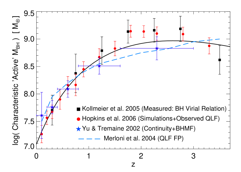
The quasar luminosity function at a given redshift has a characteristic luminosity $L_{\ast}$. Given that quasars (at least those with $L\gtrsim L_{\ast}$) are typically observed to have high Eddington ratios $\lambda\equiv L/L_{\rm Edd}\approx 0.3-0.5$ (Heckman et al., 2004; Vestergaard, 2004; McLure & Dunlop, 2004; Kollmeier et al., 2005), this $L_{\ast}$ reflects the characteristic mass of “active” BHs at that redshift, $M_{\rm BH}\approx 3.0\,\lambda^{-1}\times 10^{8}\,M_{\sun}\,(L_{\ast}/10^{13}\,L_{\sun})$. Direct observations of quasar Eddington ratios/BH masses (McLure & Dunlop, 2004; Kollmeier et al., 2005), limits from the X-ray background (Elvis et al., 2002; Cao, 2005) and BH mass functions (Soltan, 1982; Yu & Tremaine, 2002; Marconi et al., 2004; Shankar et al., 2004; Hopkins et al., 2007b), radio luminosity functions (Merloni, 2004; McLure et al., 2004), and “relic” low-luminosity Eddington ratios (Hopkins, Hernquist, & Narayan, 2005) all rule out the possibility that these BHs subsequently gain significant mass ($\gtrsim 10-20\%$ growth) after their brief “active” phase, so the $M_{\rm BH}$ above is equivalent (within its errors) to the $z=0$ BH mass of these objects. Since the relationship between BH mass and host luminosity or mass is well-determined at $z=0$ ($M_{\rm BH}=\mu\,M_{\rm gal}$ with $\mu\approx 0.001$; Marconi & Hunt 2003, Häring & Rix 2004), knowing $M_{\rm BH}(z=0)$ of a population implies, with little uncertainty, its $z=0$ host mass $M_{\rm gal}$ or luminosity.

In Figure 1, we consider the clustering of quasars as a function of redshift, evolved to $z=0$. At each redshift where the quasar clustering $b(z)$ is measured, we also know the characteristic luminosity $L_{\ast}$. Here we adopt the bolometric $L_{\ast}$ determined in the observational compilation of Hopkins et al. (2007b),

$$\log(L_{\ast}/L_{\sun})=k_{0}+k_{1}\,\xi+k_{2}\,\xi^{2}+k_{3}\,\xi^{3},$$ (2)

$$\xi\equiv\log{{\Bigl{(}}\frac{1+z}{1+z_{\rm ref}}{\Bigr{)}}}\ \ \ \ \ \ [z_{\rm ref}=2],$$ (3)

($k_{0}=13.036$; $k_{1}=0.632$; $k_{2}=-11.76$; $k_{3}=-14.25$), but for our purposes this is identical to adopting the $B$-band or X-ray $L_{\ast}$ from Ueda et al. (2003); Croom et al. (2004); Hasinger et al. (2005); Richards et al. (2006a) and converting it to a bolometric $L_{\ast}$ with a typical bolometric correction from Marconi et al. (2004); Richards et al. (2006b); Hopkins et al. (2007b). Given the conversions above, we consider the implied characteristic BH mass and, assuming little subsequent BH growth, the corresponding $z=0$ stellar mass or luminosity in a given band (here from the $M_{\rm BH}-L_{\rm host}$ relations of Marconi & Hunt, 2003). Knowing how the bias of these halos evolves to $z=0$ (Equation 1), we plot the bias as a function of stellar mass, at $z=0$, of the evolved quasar “parent” population. We compare this with observed bias as a function of stellar mass or luminosity for both early and late-type galaxies. Note that the lowest and highest-redshift bins ($z\sim 0.5$ and $z\sim 2.5$, respectively) in the Myers et al. (2007a) quasar clustering measurements are significantly affected by catastrophic redshift errors (owing to their considering all photometrically classified quasars, as opposed to just spectroscopically confirmed quasars); we follow their suggestion and decrease (increase) the clustering amplitude in the lowest (highest) redshift bin by $\sim 20\%$; excluding these points entirely, however, has no effect on our conclusions.

For reference, we show the characteristic $M_{\rm BH}$ corresponding to $L_{\ast}$ in the QLF (as defined above) as a function of redshift in Figure 2. Whether we adopt a direct conversion from the observed $L_{\ast}$ (Equation (3)) with observed Eddington ratios, as above, or invoke any of several empirical models for the QLF Eddington ratio distribution, we obtain a similar $M_{\rm BH}$. The figure illustrates the inherent factor $\lesssim 2$ systematic uncertainty in the appropriate Eddington ratios and bolometric corrections used in our conversions. These uncertainties, however, are at most comparable to the uncertainties in quasar clustering measurements. Because of this, our conclusions and comparisons are not sensitive to the exact method we use to estimate the $M_{\rm BH}$ corresponding to $L_{\ast}$ at a given redshift.

Figure 1.— Evolved clustering of quasar “descendents” (colored points) as a function of mass or luminosity, compared to clustering of early type (solid black points) and late type (open black points) galaxies of the same mass/luminosity. The measured clustering of quasars at a given $z$ (samples as labeled) is evolved in linear theory to the given observed redshift, and plotted as of function of the relic host galaxy mass/luminosity. Galaxy clustering is shown at $z=0$ from Li et al. (2006, color and morphologically-selected early types as squares and circles, respectively), Zehavi et al. (2005, color-selected; stars), Percival et al. (2006, SDSS LRGs; triangles), Norberg et al. (2002, diamonds); at $z=0.1-0.4$ from Shepherd et al. (2001, stars) and Brown et al. (2003, and references therein; diamond); at $z=0.4-0.8$ from Meneux et al. (2006, square), Phleps et al. (2005, circle), and Brown et al. (2003, and references therein; diamonds); and at $z=0.8-1.5$ from Meneux et al. (2006, square), and Coil et al. (2004, circles). Fitted lines show the best-fit bias of early type galaxies at each $z$ as a function of mass/luminosity (Norberg et al., 2001; Tegmark et al., 2004; Li et al., 2006).

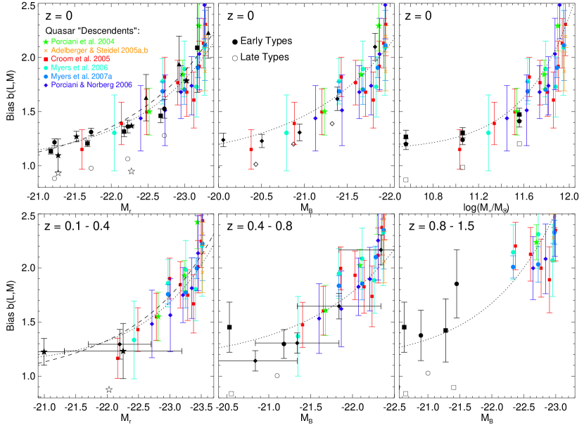
The comparison in Figure 1 is possible at any redshift, not simply $z=0$. We repeat our methodology above at several $z_{\rm obs}=0-1$, evolving the bias to $b(z_{\rm obs})$. The agreement with red galaxy clustering observed as a function of mass at each $z_{\rm obs}$ is good, at all $z\lesssim 1$. At higher redshifts, small fields in galaxy surveys limit one’s ability to measure clustering as a bivariate function of luminosity and color/morphology at the highest luminosities, where the relics of $z\sim 2-3$ quasars are expected.

Figure 2.— Characteristic “active” mass of BHs at a given redshift, i.e. the BH mass corresponding to (dominant at) $L_{\ast}$ in the QLF. Black squares adopt the virial relation BH mass determinations of Kollmeier et al. (2005). Red circles fit the observed QLF at each redshift (Hopkins et al., 2007b) to quasar light curve models (Hopkins et al., 2006b). Blue stars adopt the simplified continuity model from Yu & Tremaine (2002) and Marconi et al. (2004) given the Ueda et al. (2003) QLF. Blue dashed line (Merloni, 2004) and derives the active mass distribution from the radio and X-ray “black hole fundamental plane.” Black solid line is a fitted relation (Equations (3) & (8)). The “active” BH mass is well-defined. Adopting different estimators does not significantly alter our conclusions or comparisons in Figures 1 & 11.

3. Clustering as Function of Luminosity and Different AGN Fueling Mechanisms

The comparison in Figure 1 has one important caveat. We assumed that measurements of quasar clustering at a given redshift are representative of a “characteristic” active mass $M_{\rm BH}\propto L_{\ast}$ of the QLF. In other words, quasar clustering should be a weak function of the exact quasar luminosity, at least near $L_{\ast}$. If this were not true, our comparison would break down on two levels. First, it would be sensitive to the exact luminosity distribution of observed quasars. Second, if quasars of slightly different luminosities at the same redshift represented different BH/host masses (consequently making quasar clustering a strong function of quasar luminosity), there would be no well-defined “characteristic” active mass at that redshift.

Fortunately, Lidz et al. (2006) considered this question in detail, and demonstrated that realistic quasar light curve and lifetime models like those of Hopkins et al. (2006b) indeed predict a relatively flat quasar bias as a function of luminosity, in contrast to more naive models which assume a one-to-one correlation between observed quasar luminosity, BH mass, and host stellar/halo mass. This appears to be increasingly confirmed by direct observations, with Adelberger & Steidel (2005a); Croom et al. (2005); Myers et al. (2006, 2007a); Porciani & Norberg (2006); Coil et al. (2006b) finding no evidence for a significant dependence of quasar clustering on luminosity.

Figure 3 explicitly considers the dependence of bias on luminosity and its possible effects on our conclusions. We plot, at each of several redshifts, the observed bias of quasars as a function of luminosity. For the sake of direct comparison, all observations are converted to a bolometric luminosity with the bolometric corrections from Hopkins et al. (2007b). The QLF break luminosity $L_{\ast}$ at each redshift, estimated in Hopkins et al. (2007b), is also shown. The first thing to note is that the quasar observations with which we compare generally sample the QLF very near $L_{\ast}$, so regardless of the dependence of bias on luminosity, our conclusions are not changed. We have, for example, recalculated the results of § 2 assuming that the characteristic mass of active BHs is given by $M_{\rm Edd}({\langle}L_{\rm obs}{\rangle})$, where ${\langle}L_{\rm obs}{\rangle}$ is the mean (or median) observed quasar luminosity in each clustering sample in Figure 1, and find it makes no difference (changing the comparisons by $\ll 1\sigma$).

Figure 3.— Quasar bias as a function of quasar luminosity at each of several redshifts. Points show quasar observations from Figure 1 (same style). Open black points add the local ($z\lesssim 0.3$) observations of Constantin & Vogeley (2006, SDSS LLAGN (LINERS+Seyferts); squares), Wake et al. (2004, SDSS; star), and Grazian et al. (2004, AERQS; diamond), and the $z\sim 1$ cross-correlation measurements of Coil et al. (2006b, SDSS+DEEP2; circles). Blue dotted line shows $L_{\ast}(z)$. These are compared to various models described in the text (curves, as labeled). Models in black adopt the feedback-regulated quasar light curve/lifetime models from Hopkins et al. (2006a), others consider more simplified “light bulb” model light curves.

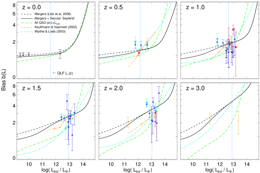
We compare the observations with various theoretical models in Figure 3. The models of Hopkins et al. (2005b) define the conditional quasar lifetime; i.e. time a quasar with a given final (relic) BH mass (or equivalently, peak quasar luminosity) spends over its lifetime in various luminosity intervals, $t_{Q}(L\,|\,M_{\rm BH})$. Since this is much less than the Hubble time at all redshifts of interest, the observed QLF ($\phi_{Q}[L]$) is given by the convolution of $t_{Q}(L\,|\,M_{\rm BH})$ with the rate at which quasars of a given relic mass $M_{\rm BH}$ are “triggered” or “turned on,”

$$\phi_{Q}(L)=\int t_{Q}(L\,|\,M_{\rm BH})\,\dot{\phi}(M_{\rm BH})\,{\rm d}\log{M_{\rm BH}},$$ (4)

where $\dot{\phi}(M_{\rm BH})$ is the rate of triggering, i.e. number of quasars formed or triggered per unit time per unit volume per logarithmic interval in relic mass. The integrand here defines the relative contribution to a given observed luminosity interval from each interval in $M_{\rm BH}$. Given the BH-host mass relation, we can convert this to the relative contribution from hosts of different masses $M_{\rm gal}$ (i.e. ${\rm d}\phi_{Q}(L)/{\rm d}\log{M_{\rm gal}}$). In detail, we assume $P(M_{\rm BH}\,|\,M_{\rm gal})$ is distributed as a lognormal about the mean correlation, with a dispersion of $0.3$ dex taken from observations (Marconi & Hunt, 2003; Häring & Rix, 2004; Novak et al., 2006) and hydrodynamical simulations (Di Matteo et al., 2005; Robertson et al., 2006a). Calculating the bias for a given relic $M_{\rm BH}$ or $M_{\rm gal}$ and observed redshift as in § 2, we can integrate over these contributions to determine the appropriately weighted mean bias as a function of observed quasar luminosity,

$${\langle}b{\rangle}(L,\,z)=\frac{1}{\phi_{Q}(L)}\,\int b(M_{\rm gal},\,z)\,\frac{{\rm d}\phi_{Q}(L)}{{\rm d}\log{M_{\rm gal}}}\,{\rm d}\log{M_{\rm gal}}.$$ (5)

Although binning by both luminosity and redshift greatly reduces the size of observed samples and increases their errors, the observations in Figure 3 confirm the predictions of Lidz et al. (2006) to the extent that they currently probe. To contrast, we construct an alternative “straw-man” model. Specifically, we compare with the naive expectation, if all quasars were at the same Eddington ratio (so-called “light-bulb” models), i.e. if there was a one-to-one correlation between observed luminosity and BH mass (and correspondingly, host mass), which produces a much steeper trend of bias as a function of luminosity and is significantly disfavored ($>4.5\,\sigma$; although from any individual sample the significance is only $\sim 2\,\sigma$). We also compare the predicted clustering as a function of luminosity from the semi-analytic models of Kauffmann & Haehnelt (2002) and Wyithe & Loeb (2003), which adopt idealized, strongly peaked/decaying exponential quasar light curves (i.e. Eddington-limited growth to a peak luminosity, then subsequent $L\propto\exp{(-t/t_{Q})}$) and therefore yield similar predictions to the constant Eddington ratio “light bulb” model (and are likewise disfavored at $>4\,\sigma$).

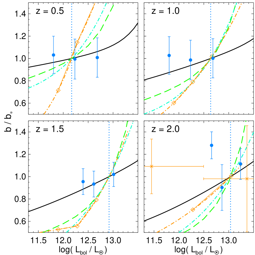
Figure 4 highlights the dependence of bias on luminosity in the observations and models by plotting the relative bias $b/b_{\ast}$ (where $b_{\ast}\equiv b(L_{\ast})$) near the QLF $L_{\ast}$, more clearly demonstrating the observational indication of a weak dependence. Alternatively, we can fit each observed sample binned by luminosity at a given redshift to a “slope,”

$$\frac{b}{b_{\ast}}=1+\frac{{\rm d}(b/b_{\ast})}{{\rm d}\log{L}}\,\log{(L/L_{\ast})},$$ (6)

the results of which are shown in Figure 5 as a function of redshift, compared to the slope (evaluated at $L_{\ast}$) predicted by the various models. At all redshifts, the observations are consistent with no dependence of clustering on luminosity, and strongly disfavor the “light-bulb” class of models (again, at $\sim 4\,\sigma$ at $z\sim 1.5-2$). This confirms the conclusions of these studies individually, particularly the most recent observations from Myers et al. (2007a) and the largest luminosity baseline observations from Adelberger & Steidel (2005a). The weak dependence predicted by the models of Hopkins et al. (2006b); Lidz et al. (2006) provides a considerably improved fit, although even it may be marginally too steep relative to the observations.

Galaxy clustering (and therefore, presumably, host halo mass) appear to be much more strongly correlated with galaxy luminosity or stellar mass (Figure 1) than with quasar luminosity (at a given redshift); i.e. the weak dependence of bias on quasar luminosity appears to be driven by variation in Eddington ratios at a characteristic “active” mass. This is also supported by comparison of quasar luminosity functions and number counts, in a semi-analytic context (Volonteri et al., 2006). We note that this is completely consistent with observations that find similar high Eddington ratios for all bright quasars, as these are confined to $L\gtrsim L_{\ast}$, (and indeed the Hopkins et al. (2006b); Lidz et al. (2006) model predictions do, at these highest luminosities, reproduce this and imply a steep trend of bias with luminosity). However, the relatively weak trend in clustering near and below $L_{\ast}$ makes our conclusions throughout considerably more robust, so long as the observed quasar sample resolves $L_{\ast}$ (true for all plotted points).

Figure 4.— As Figure 3, but showing the relative quasar bias $b/b_{\ast}$ ($b_{\ast}\equiv b(L_{\ast})$) as a function of luminosity near $L_{\ast}$ for the models and most well-constrained (Myers et al., 2007a) and largest luminosity baseline (Adelberger & Steidel, 2005a) observations, to highlight the luminosity dependence and differences between the models.

Figure 5.— The best-fit dependence of quasar bias on luminosity (${\rm d}(b/b_{\ast})/{\rm d}\log{L}$) from the observations in Figures 3 & 4 (points), compared to the dependence expected from the models (calculated at $L_{\ast}$). The observations favor little or no dependence of clustering on luminosity.

Despite the detail of the models involved, the predictions in Figure 3 are all simplified in that they model only one mechanism for quasar fueling. However, Hopkins & Hernquist (2006) (among others) predict that at low luminosities, contributions from smaller BHs in non-merging disk bulges, triggered by disk and bar instabilities, stochastic accretion, harassment, or other perturbations, are expected to dominate the “Seyfert” population. We therefore repeat our calculation, but allow different fueling mechanisms in different hosts to contribute to different quasar luminosities, according to the models of Hopkins & Hernquist (2006) and Lidz et al. (2006). Because the “Seyferts” in this particular model (Hopkins & Hernquist, 2006) are generally less massive systems at high Eddington ratio in blue, star-forming galaxies, they are less biased than merger remnants of similar observed luminosity.

The inclusion of these populations in Figure 3 does not change our conclusions near $L\sim L_{\ast}$. However it does introduce a feature, generally a sharp decrease in observed bias, at the luminosity where these secular fueling mechanisms begin to dominate the AGN population. This luminosity is typically quite low, $L\sim 10^{11}-10^{12}\,L_{\sun}$ (corresponding roughly to luminosities below the classical Seyfert-quasar division of $M_{B}=-23$). The only redshift at which the clustering of such very low-luminosity AGN has been measured is $z\lesssim 0.2$, by which point massive, gas-rich mergers are sufficiently rare that the predicted “Seyfert” population from Hopkins & Hernquist (2006) dominates the merger-triggered quasar population at all luminosities, erasing the feature indicative of a change in the characteristic host population. However, it is possible that deeper clustering observations at $z\sim 1-2$ will eventually probe these luminosities, and test this prediction.

Realistically, the luminosities of interest are sufficiently low that X-ray surveys present the most viable current probe, but with the small $\lesssim 1\,{\rm deg}^{2}$ field sizes typical of most surveys, the quasar autocorrelation function cannot be constrained to the necessary accuracy to distinguish the models. However, as proposed in Kauffmann & Haehnelt (2002), the AGN-galaxy cross-correlation presents a possible solution. For example, there are sufficient galaxies at $z\sim 1$ in the fields of surveys like e.g. DEEP2 or COMBO-17 (with field sizes $\sim 3.5\,{\rm deg}^{2}$ and $\sim 0.8\,{\rm deg}^{2}$, respectively) that the accuracy of cross-correlation measurements is limited by the number of AGN; considering the hard X-ray selected AGN samples in the CDF-N or CDF-S (with field sizes $\sim 0.01-0.5\,{\rm deg}^{2}$) from $z\sim 0.8-1.6$ would represent a factor $\sim 2-3$ increase in the number density of AGN over the Coil et al. (2006b) sample in Figure 3, while extending the AGN luminosities to a depth of $\sim 3\times 10^{9}\,L_{\sun}$ ($\sim 10^{42}\,{\rm erg\,s^{-1}\,cm^{-2}}$). The measurement of the cross-correlation between observed galaxies in these fields and deep X-ray selected faint AGN at $z\gtrsim 0.5$ does, therefore, present a realistic means to test the differences in these models at low luminosities. The observation of a feature as shown in Figure 3 should correspond to a characteristic transition in the quasar host/fueling populations.

4. Clustering of Different Populations

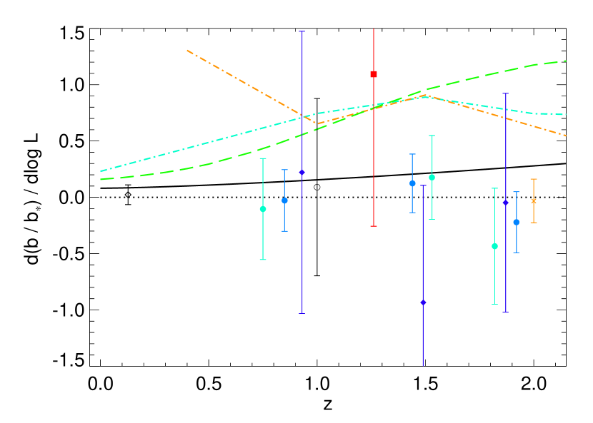
In Figure 6 we compare the observed quasar bias and correlation length as a function of redshift with the expected clustering of quasar hosts, i.e. evolving the observed bias of BH (quasar “relic”) hosts up from $z=0$. A $z=0$ elliptical galaxy or spheroid of stellar mass $M_{\rm gal}$ has a bias $b(M,\,z=0)$ shown in Figure 1, and a BH of mass $M_{\rm BH}\approx 0.001\,M_{\rm gal}$. For convenience, we adopt the analytic fit to $b(M_{\rm gal},\,z=0)$ in Li et al. (2006),

$$b(M_{\rm gal},\,z=0)/b_{\ast}=0.896+0.097\,(M_{\rm gal}/M_{\ast}),$$ (7)

where here $M_{\ast}=1.02\times 10^{11}\,M_{\sun}$ is the Schechter function “break” mass (Bell et al., 2003) and $b_{\ast}=1.2$ for red galaxies (Zehavi et al., 2005; Li et al., 2006). The progenitors of these systems therefore represent the “characteristic” active systems when the QLF characteristic luminosity $L_{\ast}(z)$ is given by $L_{\ast}(z)\approx\lambda\,L_{\rm Edd}(0.001\,M_{\rm gal})$, i.e. when these BHs dominated the $\sim L_{\ast}$ quasar population and assembled most of their mass. Evolving the local observed bias of the $z=0$ spheroids, $b(M_{\rm gal},\,z=0)$, to this redshift with Equation (1) yields the expected bias that the quasar hosts (and therefore quasars themselves) at this redshift should have, $b_{Q}(z)$. For future comparison, this is approximately given by

$$b_{Q}(z)\approx 1+0.014\,D(z)^{-1}\,10^{5.70\,x-2.30\,x^{2}-3.35\,x^{3}},$$ (8)

where $x\equiv\log{(1+z)}$ and $D(z)$ is again the linear growth factor. This expectation is plotted, with the $\sim 1\sigma$ combined uncertainties from errors in the measured QLF $L_{\ast}$ and local bias $b(M_{\rm gal},\,z=0)$, comparable to the inherent factor $\lesssim 2$ systematic uncertainty in the appropriate Eddington ratios and bolometric corrections. We also plot the corresponding correlation length $r_{0}$; because measurements of this quantity are covariant with the fitted correlation function slope $\gamma$, we renormalize the models and observations to

$$r_{0}^{\prime}\equiv 8\,h^{-1}\,{\rm Mpc}\,{\Bigl{(}}\frac{r_{0,\,\rm fit}}{8\,h^{-1}\,{\rm Mpc}}{\Bigr{)}}^{{\gamma}/{1.8}}.$$ (9)

This is similar to the non-linear $\sigma_{8}^{\rm NL}$ parameter (standard deviation of galaxy count fluctuations in a sphere of radius $8\,h^{-1}\,{\rm Mpc}$, i.e. $\sigma_{8}$ measured for an evolved density field, see Peebles, 1980), and effectively compares the amplitude of clustering at $8\,h^{-1}\,{\rm Mpc}$ with a fiducial model with $\gamma=1.8$, minimizing the covariance.

Figure 6.— Clustering of quasars as a function of redshift (colored points in left panels, black in other panels; as in Figure 1), compared to different models of possible host populations. Upper and lower panels plot bias and comoving correlation length, respectively. Solid line inverts the comparison in Figure 1, i.e. uses the estimated local clustering of red galaxies to predict the quasar clustering assuming quasars are the progenitors of present ellipticals (long dashed lines show $\sim 1\,\sigma$ range from uncertainties in local bias and observed bright quasar Eddington ratios). Dotted lines correspond to halos of constant mass (as labeled). Center panel compares this with the observed clustering of early-type galaxies (at the characteristic red galaxy $M_{\ast}$ or $L_{\ast}$ at $z\lesssim 1$; at higher redshift $b(M_{\ast})$ is not longer well determined, so various passive galaxy surveys are considered). Right panels compare with late-type galaxies.

Figure 7.— As Figure 6 (upper left), but showing only single quasar clustering measurements to highlight the significance of these comparisons from any individual survey. The two 2dF results are not independent, but use different methods to derive the quasar bias.

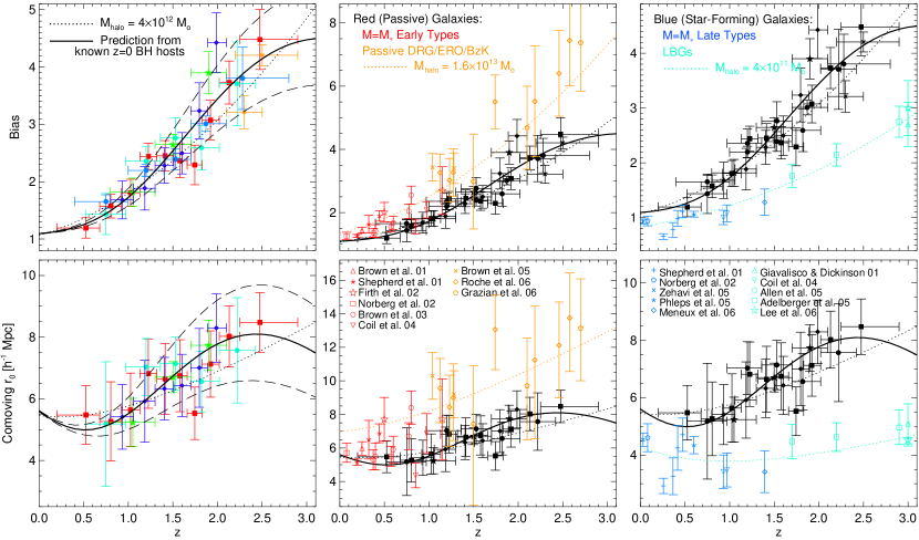
The expectation agrees well with observed quasar clustering as a function of redshift ($\chi^{2}/\nu=29.6/32$, with no free parameters). For comparison, we plot the expected clustering of halos of a fixed mass, $M_{\rm halo}\sim 4\times 10^{11}-10^{13}\,h^{-1}\,M_{\sun}$, determined in the context of linear collapse theory following Mo & White (1996), modified according to Sheth et al. (2001) and with the power spectrum calculated following Eisenstein & Hu (1999) for our adopted cosmology. As noted in most previous studies (e.g., Porciani et al., 2004; Croom et al., 2005), a constant host halo mass of a few $10^{12}\,h^{-1}\,M_{\sun}$ provides a surprisingly good fit to the trend with redshift. This empirical fit, is comparable to our expectation from elliptical populations (best-fit halo mass $3.86\times 10^{12}\,h^{-1}\,M_{\sun}$ with $\chi^{2}/\nu=28.9/31$; of course, the exact best-fit mass depends systematically on cosmology, but this conclusion is robust). There is at most a marginal trend for the halo mass to increase with redshift (for $M_{\rm halo}\propto(1+z)^{k}$, the best-fit $k=0.41\pm 0.45$; corresponding to a $\sim 50\%$ increase over the observed redshift range).

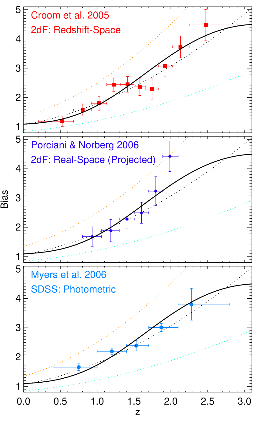
Note that the measurements shown are not all statistically independent, and the significance of this comparison will diminish if we consider any single quasar clustering measurement. Figure 7 demonstrates the same comparison, highlighting individual quasar bias measurements separately. However, the previous agreement and our conclusions are similar in all cases. As discussed by the authors, Porciani & Norberg (2006) find a somewhat higher clustering amplitude in their highest-redshift ($z\sim 2$) bin than Croom et al. (2005) studying the same sample (and higher than Myers et al. (2006) and Adelberger & Steidel (2005a) who study independent samples), but the significance of the Porciani & Norberg (2006) result is $\lesssim 2\,\sigma$.

That a constant halo mass fits the data as well as observed suggests that there may be a physical driver or triggering mechanism associated with these halos. It is suggestive that this corresponds to the “group scale;” i.e. minimum halo mass of small galaxy groups, in which galaxy-galaxy mergers are expected to proceed most efficiently. However, the redshift evolution of this threshold is not well-determined (but see Coil et al., 2006a, who find a similar “group scale” halo mass at $z=1$), nor is the rate or behavior of merging within such halos. An a priori theoretical model for the prevalence of quasars in halos of this mass is therefore outside the scope of this paper, but remains an important topic for future work.

Since it is also established, as discussed in § 2, that the characteristic mass of active BHs increases with redshift, this implies substantial evolution in the ratio of BH to host halo mass to $z\sim 2$. It is unclear how much of this may owe to evolution in the ratio of BH to host stellar mass: observational estimates imply some such evolution (e.g., Shields et al., 2005; Peng et al., 2006; Woo et al., 2006), but upper limits from evolution in stellar mass densities (Hopkins et al., 2006d) allow only a factor $\sim 2$ evolution by $z=2$. Therefore, there might also be at least some increase with redshift in the characteristic ratio of stellar to halo mass. Future constraints from halo occupation models or galaxy clustering at high redshifts will be valuable in breaking this degeneracy, and potentially provide important clues to galaxy assembly histories.

We contrast these predictions with two extremely simple models. In the first, quasar activity is an unbiased tracer of dark matter, i.e. $b(z)=1$. This does, after all, appear true at $z=0$ (Wake et al., 2004; Grazian et al., 2004; Constantin & Vogeley, 2006). This is immediately strongly ruled out: there is an unambiguous trend that higher-redshift quasars are more strongly biased (as noted in essentially all observed quasar correlation functions).

Next, we consider the possibility that quasars live in the same halos at all redshifts. This is equivalent to some “classical” interpretations of pure luminosity evolution in the QLF (e.g., Mathez, 1976); i.e. that quasars are cosmologically-long lived (although other observations demand a lifetime $\lesssim 10^{7}$ yrs; e.g. Martini, 2004, and references therein), and dim from $z=2$ to the present. It is also equivalent to saying that quasars are triggered, even for a short time, in the same objects over time (e.g., stochastically or by some cyclic mechanism). In this case, the quasar lifetime can still be short (with a low “duty cycle” $\delta\sim 10^{-3}$), although Eddington ratios must still tend to increase with redshift. Then, the halo bias evolves as Equation (1), from a $z=0$ value $b(0)\sim 1.0-1.2$ (Norberg et al., 2002). Although this model is qualitatively consistent with some quasar observations, it is not nearly sufficient to explain the evolution of clustering amplitude with redshift and is ruled out at very high ($>10\,\sigma$) significance. As noted in previous studies of quasar clustering (Croom et al., 2005), quasars at different redshifts must reside in different parent halo populations; quasars cannot, as a rule, be long lived or recurring/episodic/cyclic (although this does not apply to very low-accretion rate activity, perhaps associated with “radio modes”; see e.g. Hopkins, Hernquist, & Narayan 2005).

Rather than a uniform population of halos at all redshifts, what if quasars uniformly sample observed galaxy populations? It is, for example, easy to modify the above scenario slightly: quasars are cosmologically long-lived or uniformly cyclic/episodic, but only represent the present/extant population of BHs (equivalently, the present population of spheroids). In this case, quasar correlation functions should uniformly trace early-type correlations at all redshifts.

Figure 6 compares observed early-type/red galaxy clustering as a function of redshift with that measured for quasar populations. At low redshifts $z\lesssim 1$, both mass functions and clustering as a function of mass/luminosity are reasonably well-determined, so we plot clustering at the characteristic early-type (Schechter function) $M_{\ast}$ or $L_{\ast}$. At higher redshift, caution should be used, since this characteristic mass/luminosity is not well determined, and so we can only plot clustering of observed massive red galaxies (which, given the observed dependence of clustering amplitude on mass/luminosity and color, may bias these estimates to high $b(z)$ if surveys are not sufficiently deep to resolve $M_{\ast}$ or $L_{\ast}$). There is also the additional possibility that the poorly known redshift distribution of these objects may introduce artificial scatter in their clustering estimates. Bearing these caveats in mind, the clustering of quasars and red galaxies are inconsistent at high ($>6\sigma$) significance. Quasars do not uniformly trace the populations of spheroids/BHs which are “in place” at a given redshift. Note, however, that in this comparison the systematic errors almost certainly dominate the formal statistical uncertainties, so the real significance may be considerably lower.

An alternative possibility is that BH growth might uniformly trace star formation. In this case, quasar clustering should trace the star-forming galaxy population. Figure 6 compares observed late-type/blue/star-forming galaxy clustering as a function of redshift with that observed for quasar populations. Again, at $z\lesssim 1$ we plot clustering at the characteristic $M_{\ast}$ or $L_{\ast}$. At higher redshift we can only plot “combined” clustering of observed star-forming populations (generally selected as Lyman-break galaxies); again caution is warranted given the known dependence of clustering on galaxy mass/luminosity (for LBGs, see Allen et al., 2005). In any case, the clustering is again inconsistent at high ($>10\sigma$) significance. Quasars do not uniformly trace star-forming galaxies. This appears to be contrary to some previous claims (e.g., Adelberger & Steidel, 2005a); however, in most cases where quasars have been seen to cluster similarly to blue galaxies, either faint AGN populations (not $\sim L_{\ast}$ quasars) or bright ($\gg L_{\ast}$) blue galaxies were considered. Indeed, quasars do cluster in a manner similar to the brightest blue galaxies observed at several redshifts (e.g., Coil et al., 2006c; Allen et al., 2005, at $z\sim 1$ and $z\gtrsim 2$, respectively). This should not be surprising; since quasars require some cold gas supply for their fueling, they cannot be significantly more clustered than the most highly clustered (most luminous) population of galaxies with that cold gas. Again, this highlights the fact that the real systematic issues in this comparison probably make the significance considerably less than the formal $\sim 10\,\sigma$ seen here.

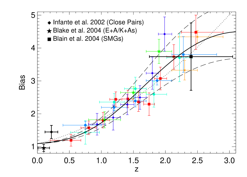
We would also like to compare quasar clustering directly to the clustering of gas-rich (luminous) mergers. Figure 8 attempts to do so, using available clustering measurements for likely major-merger populations. At low redshifts, Blake et al. (2004) have measured the clustering of a large, uniformly selected sample of post-starburst (E+A or K+A) elliptical galaxies in the SDSS, which from their colors, structural properties, and fading morphological disturbances (e.g., Goto, 2005, and references therein) are believed to be recent major merger remnants. Infante et al. (2002) have also measured the large-scale clustering of close galaxy pairs selected from the SDSS at low redshift. At high redshift, no such samples exist, but Blain et al. (2004) have estimated the clustering of a moderately large sample of spectroscopically identified sub-millimeter galaxies at $z\sim 2-3$, for which the similarity to local ULIRGs in high star formation rates, dust content, line profiles, and disturbed morphologies suggests they are systems undergoing major, gas-rich mergers (e.g., Pope et al., 2005, 2006; Chakrabarti et al., 2006, and references therein). The clustering of these populations is consistent at each redshift with observed quasar clustering (see also Hopkins et al., 2007a). This is contrary to the conclusions of Blain et al. (2004), but they compared their SMG clustering measurement with earlier quasar clustering data (Croom et al., 2002) below their median redshift $z\sim 2.5$. Figure 8 demonstrates that the dependence of quasar clustering on redshift is such that at the same redshifts, the two agree very well. However, given the very limited nature of the data, and the lack of a uniform selection criteria for ongoing or recent mergers at different redshifts, we cannot draw any strong conclusions from the direct merger-quasar clustering comparison alone.

Figure 8.— As Figure 6, but comparing observed quasar clustering (colored points) as a function of redshift to that various populations usually associated with galaxy mergers (black points): post-starburst (E+A/K+A) galaxies, close galaxy pairs, and sub-millimeter galaxies.

Although quasars do not appear to trace star-forming galaxies, Adelberger et al. (2005, and references therein) have shown that the star formation rates, clustering properties, and number densities of high-redshift LBGs suggest they are the progenitors of present-day ellipticals. To the extent that quasars are also the progenitors of ellipticals (but with a larger clustering amplitude at a given redshift compared to LBGs), this suggests a crude “straw-man” outline of an evolutionary sequence with time, from LBG to quasar to remnant elliptical galaxy. Knowing how the clustering properties of halos hosting LBGs with a given observed bias at some redshift $z_{\rm LBG}$ will subsequently evolve, we can determine the redshift $z_{Q}$ at which this matches observed quasar clustering properties. This offset, if LBGs and quasars are indeed subsequent progenitor “phases” in the sequence of evolution to present day ellipticals, defines the “duration” of the LBG “phase” or time between LBG and quasar “stages.”

Figure 9 considers this in detail. We show the observed clustering of quasars and LBGs from Figure 6, with curves illustrating the subsequent clustering evolution of the LBG host halos observed at $z=1$, $z=2$, and $z=3$. These correspond to the characteristic observed quasar clustering at $z=0.4$, $z=1.0$, and $z=1.3$, respectively. Thus, halos of the characteristic LBG host halo mass at $z=3$ will grow to the characteristic quasar host mass at $z=1.3$, and so on. We also show the physical time corresponding to this offset, calculated from the observed LBG clustering at various redshifts and the best-fit estimate of the LBG host mass $\sim 4\times 10^{11}\,h^{-1}\,M_{\sun}$, and this time divided by the Hubble time (age of the Universe) at the “quasar epoch” $z_{Q}$. Interestingly, this implies that objects characteristically spend $\sim 3-4$ Gyr ($\sim 1/2\,t_{H}$ at the redshifts of interest) in the “LBG phase.” This may reflect the time for dark matter halos to grow from the characteristic LBG mass, at which star formation and the conversion of mass to light appears to be most efficient (e.g., White & Rees, 1978) to the typical quasar host mass; but it is also possible that associated physical processes related to quasar fueling or the termination of star formation set this timescale. If quasars are triggered in major mergers, this rather large time offset (as opposed to the typical $\sim 100\,$Myr delay between starburst and quasar in major merger simulations, Di Matteo et al., 2005) implies that LBGs are themselves not primarily driven in major mergers. A similar conclusion was recently reached by Law et al. (2006) from direct analysis of LBG morphologies at $z\sim 2-3$. This conclusion and the LBG clustering in Figure 9 (Wechsler et al., 2001) are broadly consistent with the expectations of semi-analytic models (Somerville et al., 2001) which argue LBGs are driven largely by “collisional” minor merging.

Figure 9.— Upper: Clustering of quasars and star-forming galaxies, as in Figure 6. Solid green lines show the subsequent evolution of the clustering of the star-forming galaxy halos from $z=1,\,2,\,3$. Middle: Time delay between the star-forming or LBG phase and “quasar” epoch, defined as the time after the observed redshift of each LBG population at which its evolved clustering will match that of the observed quasar population. Points as in upper panel, with data from Ouchi et al. (2004, cyan inverted triangles) added at $z>4$. Dashed and dotted lines show time for halos of mass $\sim 4\times 10^{11}\,h^{-1}\,M_{\sun}$ (the typical LBG host mass) at each redshift to reach $\sim 4\times 10^{12}\,h^{-1}\,M_{\sun}$ (dotted) or the (weakly redshift-dependent) halo mass defined by our best-fit trend in the upper panel (solid). Lower: As the middle panel, but the time shown is as a fraction of the Hubble time at the “quasar” epoch.

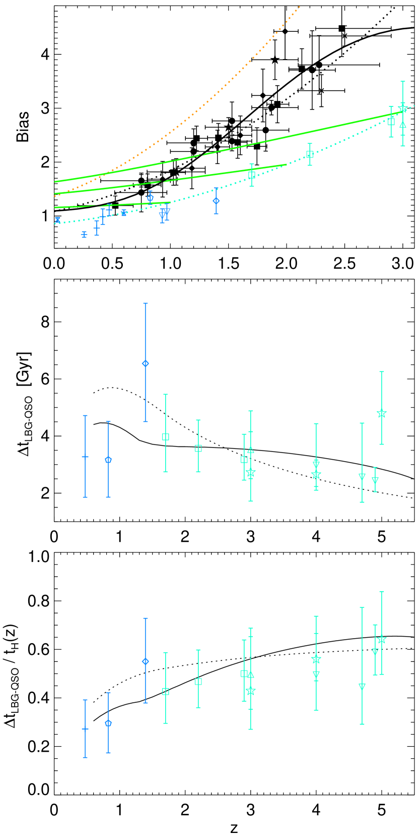
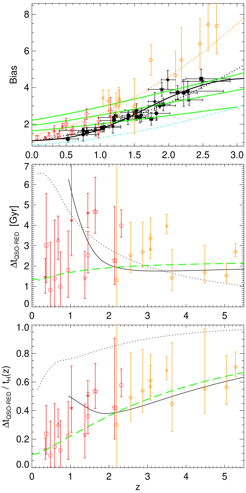
We can also use this approach to determine the time between the “quasar” and red/elliptical phases in this evolutionary sequence. Figure 10 shows this, in the style of Figure 9, where the redshift shown in the middle and lower panels refers to the redshift of the observed quasar population, and the time to the delay at which their evolved clustering matches that measured for the red galaxy population. Note that the continuous curves calculated in the middle and lower panels assume the red galaxy clustering is well-fitted by the plotted (upper panel) constant halo mass $\sim 1.6\times 10^{13}\,h^{-1}\,M_{\sun}$ curve; this is, in fact, not a very good approximation at low redshifts, hence these curves diverge below $z\sim 1-2$ from the times calculated from the actual red galaxy clustering measurements.

In the lower panels, we also plot the time for “burst-quenched” star formation history models adapted from Harker et al. (2006) to redden to a typical constant “red galaxy” threshold rest-frame color $U-B>0.35$. These model star formation histories assume a constant star formation rate until $1\,$Gyr before the “quasar epoch,” then a factor $5$ enhanced star formation rate for this $1\,$Gyr, at which point star formation ceases. Essentially, this yields a useful toy model for “quenching,” if indeed the triggering of quasars is associated with the formation of ellipticals or termination of star formation (the pre-quenching enhancement being an approximation to, e.g., merger-induced star formation enhancements), which Harker et al. (2006) demonstrate yields a reasonable approximation to the observed mean color, number density, and Balmer H$\delta_{\rm F}$ absorption strength evolution of red galaxies. The predicted time for such quenched star formation histories to redden to typical red galaxy colors agrees well with the time estimated from clustering here at all redshifts; i.e. the color and halo mass evolution of these systems are consistent with reasonable star formation histories in which quasar activity is associated with “quenching” or the termination of star formation.

Figure 10.— As Figure 9, but instead showing the time from the “quasar phase” to the “red galaxy” phase implied by the observed clustering of both populations. Green long-dashed lines in the middle and lower panels show the time required for the “burst-quenched” star formation history models from Harker et al. (2006) (which yield a good empirical approximation to the buildup and mean color evolution of red galaxies) to redden to a threshold $U-B>0.35$.

We have estimated the time offsets in Figures 9 & 10 from a direct comparison of the observed clustering. Instead, one might imagine adopting the implied halo mass ($\sim 4\times 10^{11}\,h^{-1}\,M_{\sun}$) at the “star-forming” phase and using extended Press-Schechter (EPS) theory to calculate the average time for a typical progenitor halo of this mass at each observed redshift to grow to the implied quasar host halo mass ($\sim 4\times 10^{12}\,h^{-1}\,M_{\sun}$). We discuss this in greater detail in § 5, and show that it has no effect on our conclusions. For the purposes here, adopting this methodology (specifically, calculating the evolution of the “main branch” progenitor halo mass with redshift following Neistein et al. (2006) in our adopted cosmology) systematically increases the inferred time delays (points) in Figure 9 by $\sim 1-2$ Gyr and those in Figure 10 by $\sim 0.5-1$ Gyr, but does not significantly change the plotted trends or comparisons.

So, this leaves us with the following suggested empirical picture of galaxy evolution. Galaxies form and experience a typical “star forming” or LBG epoch, with maximal efficiency around a characteristic halo mass of a few $\sim 10^{11}\,h^{-1}\,M_{\sun}$. Growth continues, presumably via normal accretion, minor mergers, and star formation, for roughly half a Hubble time, until systems have growth to a characteristic halo mass $\sim 4\times 10^{12}\,h^{-1}\,M_{\sun}$. At this point, some mechanism (for example, a major merger, as this may be the characteristic scale at which the host halo grows large enough to host multiple “large” star-forming systems) triggers a short-lived “quasar” phase, drives a morphological transformation from disk to spheroid, and terminates star formation. About $\sim 1-2$ Gyr after this, the host halos have grown to $\sim 10^{13}\,h^{-1}\,M_{\sun}$ and the spheroids have reddened sufficiently to join the typical “red galaxy” population. They then passively evolve (although they may experience some gas-poor or “dry” mergers) to $z=0$, satisfying observed correlations between BH and spheroid properties. Although individual BHs can, in principle, gain significant mass from “dry” mergers (see, e.g. Malbon et al., 2006), this cannot (by definition) add to the total mass budget of BHs, which must be built up via accretion. Note that this is only a rough conception outline of an “average” across populations and should not be taken too literally. Different systems will undergo these processes at different times, and (possibly) via different mechanisms. Still, this provides a potentially useful framework in which to interpret these observations.

5. Age-Mass Relations and Clustering

In Figure 11, we compare the mean age of BHs of a given $z=0$ mass with that of the stellar population of their hosts. At a given redshift, the characteristic QLF luminosity $L_{\ast}(z)$ and corresponding characteristic “active” mass $M_{\rm BH}$ from Figure 2 define the epoch of growth of BHs of that mass. The typical “age” of BHs of that mass will be the time since this epoch. In detail, Equation (4) relates the observed QLF to the rate at which BHs of a given relic mass are formed as a function of redshift. We adopt the fits to this equation given in Hopkins et al. (2007b), which use the model quasar lightcurves determined in Hopkins et al. (2006a, b) to calculate the time-averaged rate of formation of individual BHs as a function of mass and redshift, to estimate the median age (peak in rate of formation/creation of such BHs as a function of time) and $25-75\%$ interquartile range in “formation times.” This introduces some model dependence, but as discussed in § 2 a similar result is obtained using very different methodologies, including purely empirical, simplified models (Yu & Tremaine, 2002; Merloni, 2004; Marconi et al., 2004; Shankar et al., 2004), or direct calculation from observed Eddington ratio distributions (Vestergaard, 2004; McLure & Dunlop, 2004; Kollmeier et al., 2005).

In any case, we recover the well-known trend that the more massive BHs are formed at characteristically earlier times (Salucci et al., 1999; Yu & Tremaine, 2002; Ueda et al., 2003; Heckman et al., 2004; Hasinger et al., 2005; Merloni, 2004; Marconi et al., 2004; Shankar et al., 2004; McLure & Dunlop, 2004; Kollmeier et al., 2005). This is not surprising, as most massive BHs must be in place by $z\sim 2$ to power the brightest quasars, and these objects are generally “dead” by low redshift (with lower-mass objects dominating the local QLF, e.g. Heckman et al., 2004).

Figure 11.— Left: Upper panel shows the mean $z=0$ age (lookback time to the mean “formation epoch”) of BHs as a function of mass (black solid line, dashed lines show $25\%-75\%$ quartile ranges), compared to the stellar population age of their hosts. Ages of spheroids as a function of mass (with $M_{\rm BH}=\mu\,M_{\rm gal}$) are shown (colored points) from Nelan et al. (2005, NFPS; red squares), Gallazzi et al. (2006, SDSS; blue stars), Thomas et al. (2005, orange circles; “field” subsample). Errors show the dispersion in ages at a given mass. Lower panel uses this age to predict quasar clustering as a function of redshift; i.e. assuming the “quasar epoch” of spheroids of a given mass is associated with the termination of star formation (black lines, as labeled; colored points show observed quasar clustering as in Figure 6). Center: Same, for ages of host disks; ages from $\tau$-model fits of Bell & de Jong (2000, red) and Gavazzi et al. (2002, orange) (the offset between them owes to the choice of initial time in the $\tau$-model). Solid lines asumme $M_{\rm BH}\propto M_{\rm bulge}$, dotted $M_{\rm BH}\propto(M_{\rm disk}+M_{\rm bulge})$. Dashed lines re-calculate the age for a single-burst SFH. Lower panel is as lower left, assuming quasar activity is associated with the star formation epoch (as labeled). Right: Blue (solid) line shows the “all progenitor” age (DM “downsizing” from Neistein et al., 2006), red (dashed) the age of the main progenitor halo, and green (dotted) the time when halo crossed the “quenching” mass from Dekel & Birnboim (2006). Lower panel as lower left, assuming quasar age is equal to the halo age as labeled.

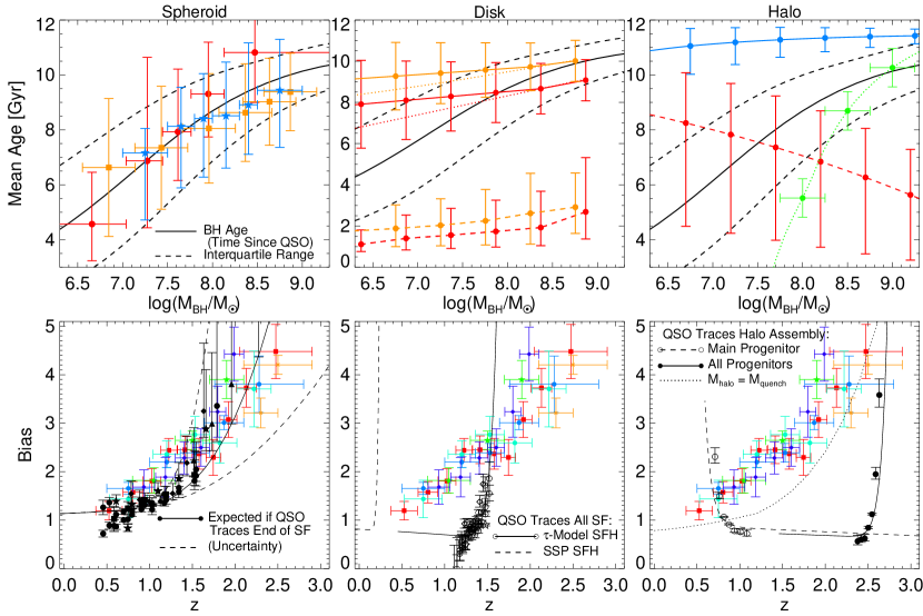
Given a BH mass, we can compare with the observationally determined age of the typical host galaxy (with $M_{\rm BH}=\mu\,M_{\rm gal}$). First, we consider early-type hosts, specifically the stellar ages of host spheroids of BHs at each mass $M_{\rm BH}$. The mean ages (and dispersion about that mean) of ellipticals as a function of stellar mass have been estimated in a number of studies, recently for example by Gallazzi et al. (2005, 2006), who fit SDSS spectra (line indices) and photometry for $\sim 175,000$ local galaxies to various realistic star formation histories, including a mix of continuous and/or starbursting histories while allowing mass, total metallicity, and abundance ratios to freely vary. They quote $r$-band light-weighted ages, which for our purposes are effectively equivalent to the ages determined by fitting a single stellar population (SSP) or “single burst” model to observed spectra, and indeed agree very well with best-fit SSP ages from similar SDSS samples (Clemens et al., 2006; Bernardi et al., 2006) and previous studies (Jørgensen, 1999; Trager et al., 2000; Kuntschner et al., 2001; Caldwell et al., 2003; Bernardi et al., 2005; Nelan et al., 2005; Thomas et al., 2005; Collobert et al., 2006, for a review see Renzini 2006) as a function of elliptical stellar mass. A similar result is also obtained independently by Treu et al. (2005) and di Serego Alighieri et al. (2006) from studies of the the fundamental plane evolution of early-type galaxies. Note that the error bars shown are the measured dispersions in the population about the mean age at a given mass, not the uncertainties in the mean ages themselves (which are smaller; $\sim 0.2$ Gyr statistical, $\sim 1$ Gyr systematic; see Nelan et al., 2005). The agreement between BH and host stellar ages is good at all masses; both the trend and dispersion (interquartile or $\pm 1\sigma$ range) about it are similar ($\chi^{2}/\nu\sim 8/17$ for a direct comparison).

If the age of its stellar populations is indicative of when the “quasar epoch” occurred in a given host, then, without making any assumptions about the masses of black holes or quasar Eddington ratios, we can use the mean age of stellar populations to predict quasar clustering. In this scenario, ellipticals of mass $M$, with mean age $t_{\rm host}$, would represent the population “lighting up” as quasars at a lookback time of $t_{\rm host}$, and so the quasar bias at that lookback time should be the local bias of ellipticals of mass $M$ (Equation 7), evolved to the appropriate lookback time $t_{\rm host}$ with Equation (1). Figure 11 compares this expectation with the observed quasar bias as a function of redshift. Despite the very simple nature of this model, which ignores both the range of ages at a given $M$ and, similarly, the range in host masses at a given time, the agreement is reasonable. Including the dispersion in ages, i.e. modeling the age distribution at each $M_{\rm BH}$ as a Gaussian with the observed scatter, improves the agreement and yields a nearly identical prediction of bias as a function of redshift to that in Figure 6 (solid black line).

We can of course repeat these exercises for other possible “host” populations. We next consider correlations with the star formation histories of late-type or star-forming host galaxies – i.e. the possibility that quasar activity is generically associated with star formation. The observed star formation histories are similarly estimated, generally by fitting to exponentially declining models ($\tau$-models; star formation rate $\dot{M}\propto\exp{[-(t-t_{i})/\tau]}$ since an initial cosmic time $t_{i}$). Specifically, we consider the fits of late-type ages as a function of stellar mass from Bell & de Jong (2000) and Gavazzi et al. (2002) (consistent with Jansen et al., 2000; Bell et al., 2000; Boselli et al., 2001; Kauffmann et al., 2003a; Pérez-González et al., 2003; Brinchmann et al., 2004; MacArthur et al., 2004; Gallazzi et al., 2005). The mass-weighted age is calculated from the model SFR (see Bell & de Jong, 2000, Equation 3). Bell & de Jong (2000) and Gavazzi et al. (2002) technically quote the age and metallicity as a function of $K$ and $H$ band absolute magnitudes, respectively, but given their quoted best-fit stellar population models at each luminosity, it is straightforward to calculate the corresponding mass-to-light ratios ($M/L_{K}$ and $M/L_{H}$) and convert the observed luminosities to total stellar masses. To convert to a corresponding BH mass, we consider first a uniform application of the local BH-host mass relation, i.e. assuming BH mass is correlated with total stellar mass, and second determining the mean bulge-to-disk ratio for a given total late-type stellar mass or luminosity (see Fukugita et al., 1998; Aller & Richstone, 2002; Hunt et al., 2004, for the appropriate mean $B/T$ for different masses/luminosities) and assuming BH mass is correlated with the bulge mass only. Because the trend of age as a function of stellar mass is weak, considering the total mass or bulge mass makes little difference in our comparison, and we subsequently consider the observationally preferred correlation between BH and bulge mass.

The mean age of a given population derived from different model star formation histories will, of course, be weighted differently. To show the systematic effects of such a choice, we roughly estimate the equivalent age from a single burst or SSP model. We calculate the $z=0$ observed $(B-V)$ color at each mass from the mean best-fit $\tau$ models, and then calculate the corresponding age for the same $(B-V)$ of a single burst model (of the same metallicity as a function of mass) from the models of Bruzual & Charlot (2003) with a Salpeter (1955) IMF. Although most of the observations above find this SSP approximation is not good for star-forming galaxies, it illustrates an important point. The SSP ages are weighted towards the youngest, bluest stellar populations – essentially functioning as an indicator of the most recent epoch of significant star formation, and are therefore quite young ($\lesssim 2\,$Gyr; similar to the typical time since recent low-level starbursting activity found in late-types with the more realistic star formation histories in Kauffmann et al., 2003a). However, the trend as a function of mass is unchanged and the overall agreement is worse. Therefore, while the systematic effects here are substantially larger than the measurement errors in mean age as a function of mass, they cannot remedy the poor agreement with the ages of BH populations.

We again use this age as a function of total/bulge mass, and the observed clustering of late-type galaxies from Figure 1 at $z=0$, to estimate what the quasar bias as a function of redshift should be, if these systems were the hosts of quasars and their quasar epoch were associated with the age of their stellar populations. The predictions are inconsistent with the observations at high significance ($>4.5\sigma$), regardless of the exact age adopted ($\tau$-model or SSP). In fact, the predicted clustering as a function of redshift is highly unphysical (owing to the fact that there is relatively little difference in ages, but strong difference in clustering amplitudes from the least to most massive disks). Ultimately, this demonstrates that the hypothesis that quasar activity generically traces star formation is unphysical. This is also supported by the fact that the integrated global star formation rate and quasar luminosity density evolve in a similar, but not identical manner from $z\sim 0-6$ (e.g., Merloni et al., 2004).

We next consider the the possibility that quasar activity traces pure dark matter assembly processes – i.e. that the buildup of BHs in quasar phases purely traces the formation of their host halos. Given the local BH-host stellar mass relation from Marconi & Hunt (2003), and the typical halo mass as a function of early-type hosted galaxy mass calibrated from weak lensing studies by Mandelbaum et al. (2006), we obtain the mean host halo mass as a function of BH mass (mean $M_{\rm halo}\sim 4\times 10^{4}\,M_{\rm BH}$; although the relation is weakly nonlinear). For our adopted cosmology, we then calculate the mean age (defined as the time at which half the present mass is assembled) of the main progenitor halo for $z=0$ halos of this mass. Error bars are taken from an ensemble of random EPS merger trees following Neistein et al. (2006). Knowing the mass of a halo at a given redshift, we calculate its clustering following Mo & White (1996) as in § 4, and use this combined with the mean ages to estimate the expected quasar clustering as a function of redshift if quasars were associated with this formation/assembly of the main progenitor halo. Although the exact age will depend on cosmology and the adopted “threshold” mass fraction at which we define halo “age,” the result is the same, namely we recover the well-known hierarchical trend in which the most massive objects are youngest, in contradiction with quasar/BH ages.

However, Neistein et al. (2006) have pointed out that the mean assembly time, considering all progenitor halos, can exhibit so-called “downsizing” behavior. We therefore follow their calculation of the mean age of all progenitors as a function of $z=0$ halo (and corresponding BH) mass, and also use this to estimate quasar clustering as a function of redshift. Again, although the systematic normalization depends somewhat on our definitions, it is clear that the recovered “downsizing” trend is, as the authors note, a subtle effect, and not nearly strong enough (inconsistent at $>10\sigma$) to explain the downsizing of BH growth. Again, the absolute value of the age obtained can be systematically shifted by changing our definition of halo “assembly time,” but the trend is not changed and significance of the disagreement with BH formation times is still high.

Certain feedback-regulated models predict that black hole mass should be correlated with halo circular velocity (as $M_{\rm BH}\propto v_{c}^{5}$ or $\propto v_{c}^{4}$; Silk & Rees, 1998; Wyithe & Loeb, 2003), rather than halo mass. To consider this, we have re-calculated the “all progenitor” and “main progenitor” ages, but instead adopted the time at which the appropriate power of the circular velocity ($v_{c}^{5}$ or $v_{c}^{4}$) reaches half the $z=0$ value. Because, for a given halo mass, $v_{c}$ is larger at higher redshift, this systematically shifts both ages to higher values, but the trends are similar. In each case the resulting ages disagree with the quasar/BH ages at even higher significance.

Alternatively, some models (Birnboim & Dekel, 2003; Binney, 2004; Kereš et al., 2005; Dekel & Birnboim, 2006) suggest that a qualitative change in halo properties occurs at a characteristic mass, above which gas is shock-heated and cannot cool efficiently, forming a quasi-static “hot accretion” mode in which quasar feedback can act efficiently. Although there is no necessary reason why quasar activity should be triggered by such a transition, its posited association with quasar feedback leads us to consider this possibility.

Knowing the mean $z=0$ halo mass for a given $M_{\rm BH}$, we plot the age at which the main progenitor halo mass surpassed the critical “quenching” mass defined as a function of redshift in Dekel & Birnboim (2006). Since this amounts to a nearly constant characteristic halo mass $\sim\times 10^{11}-10^{12}\,M_{\sun}$, the expected quasar clustering as a function of redshift is not unreasonable (see Figure 6; there is a systematic offset, but this is sensitive to the adopted cosmology). However, this model actually predicts too steep a trend of age with mass (inconsistent at $>6\sigma$). The ages of the most massive systems are reasonable (which, in comparison to the ages of ellipticals, has been widely discussed; Dekel & Birnboim, 2006; Croton et al., 2006; De Lucia et al., 2006), but the host halo of a typical $\sim 10^{8}\,M_{\sun}$ BH (i.e. Schechter $M_{\ast}$) crosses the threshold halo mass a mere $\sim 5$ Gyr ago, predicting, in this simple model, that these BHs should have been the characteristic active systems at $z\sim 0.5$ instead of the observed $z\sim 1.2-1.5$. At lower masses, the mean $z=0$ halos are only just at, or are still below, this critical halo mass. Given the scatter in the BH-host mass relations, there will be some BHs of these smaller masses living in larger halos which have already crossed the “quenching” mass, but the age distribution will still be one-sided and weighted to very young ages. To match the observed age trend, there must, in short, be some process which can trigger quasar activity at other halo masses before they cross the “quenching” threshold.

Figure 12.— Observed clustering of quasars, compared to that inferred from their $z=0$ early-type hosts if the termination of star formation is coincident with quasar activity (as lower left panel in Figure 11). Left: Our standard methodology is used to empirically evolve the clustering of local systems (black points) to the redshifts shown. Right: Instead, using the full EPS formalism and estimated $b(M_{\rm halo},\,z)$ to evolve the clustering of local systems. Differences owing to the choice of methodology are small at the halo masses of interest.

Finally, we note that in evolving the clustering of local systems “up” in redshift in the lower panels of Figure 11, there might be some ambiguity (if, for example, a given $z=0$ halo is assembled from many progenitor high-redshift halos with significantly different properties). The simple evolution predicted by Equation (1) is derived from pure gravitational motions, and therefore as applied moving “backwards” in time represents an effective “mean” bias of the progenitors of the $z=0$ system (see Fry, 1996). To the extent, however, that there is a dominant progenitor halo at a given redshift and many smaller halos which will be accreted by the “main” halo, it is the properties of the main progenitor which are of interest here.

We therefore consider a completely independent approach to empirically compare the clustering measurements shown, which attempts to capture these subtleties. Given a $z=0$ population, we can estimate its characteristic host halo mass either directly from the measurements of Mandelbaum et al. (2006), or indirectly by matching the observed bias (with bias as a function of halo mass calculated for the adopted cosmology following Mo & White (1996) and Sheth et al. (2001) as in § 4). Following Neistein et al. (2006), we then calculate the mass of the main progenitor halos of this $z=0$ mass, as a function of redshift (i.e. the highest-mass “branch” of the EPS merger tree at each redshift). At the redshift of interest (e.g. appropriate lookback time, for the comparisons in the lower panels of Figure 11), we then calculate the expected bias for halos of this main progenitor mass.

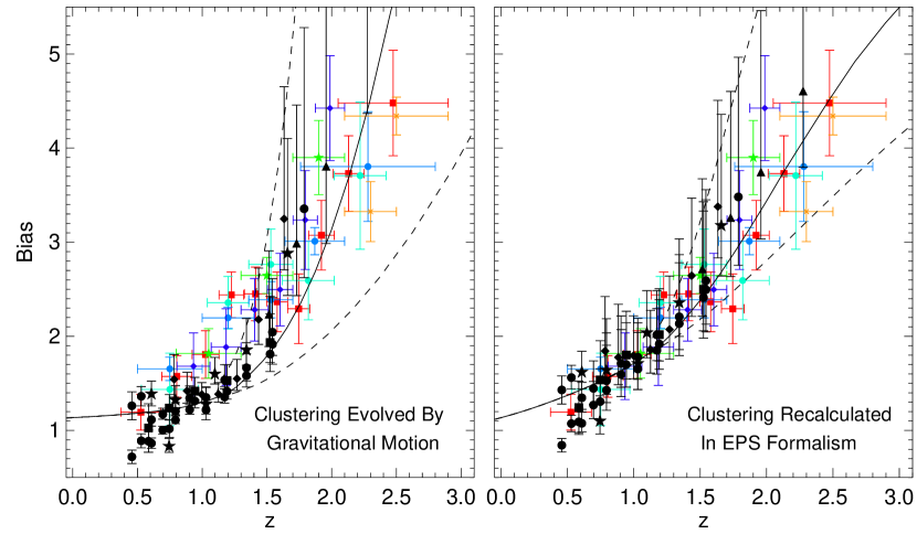
Figure 12 reproduces the lower-left comparison in Figure 11 (the expected clustering of elliptical progenitors at the times determined by their stellar population ages), using both our previously adopted methodology and this revised estimation. The latter method has the advantage, as noted above, of accounting for the difference between the main progenitor and smaller, accreted systems. The approach, however, suffers from certain inherent ambiguities in Press-Schechter theory. For example, the calculated evolution is not necessarily time-reversible, and the clustering properties are assumed to be a function of halo mass alone, which recent high-resolution numerical simulations suggest may not be correct (e.g., Gao & White, 2006; G. Harker et al., 2006; Wechsler et al., 2006). In particular, if quasars are triggered in mergers (i.e. have particularly recent halo assembly times for their post-merger halo masses), then they may represent especially biased regions of the density distribution. Unfortunately, it is not clear how to treat this in detail, as there remains considerable disagreement in the literature as to whether or not a significant “merger bias” exists (see, e.g. Kauffmann & Haehnelt, 2002; Percival et al., 2003; Furlanetto & Kamionkowski, 2006). Furthermore the distinction between galaxy-galaxy and halo-halo mergers (with the considerably longer timescale for most galaxy mergers) means that it is not even clear whether or not, after the galaxy merger, there would be a significant age bias. In any case, most studies suggest the effect is quite small: using the fitting formulae from Wechsler et al. (2002, 2006), we find that even in extreme cases (e.g. a $M\gg M_{\rm vir}$ halo merging at $z=0$ as opposed to an “average” assembly redshift $z_{f}\approx 6$) the result is that the “standard” EPS formalism underestimates the bias by $\approx 30\%$. For the estimated quasar host halo masses and redshifts of interest here, the maximal effect is $\lesssim 10\%$ at all $z=0-3$, much smaller than other systematic effects we have considered. This is consistent with Gao & White (2006) and Croton et al. (2007) who find that “assembly bias” is only important (beyond the $10\%$ level) for the most extreme halos or galaxies in their simulations.

In practice, Figure 12 demonstrates that, for the halo masses of interest here, the two methods yield very similar results. This is reassuring, and owes to the fact that the differences from the choice of methodology discussed above are important only at very high or very low halo masses, where for example the clustering of small halos which are destined to be accreted as substructure in clusters ($\gtrsim 10^{15}\,h^{-1}\,M_{\sun}$) will be very different from the clustering of similar-mass halos in field or void environments. Alternatively, one can think of the EPS approach as attempting to account for the possibility that bias is a non-monotonic function of mass (e.g. rising galaxy bias at very low luminosities, Norberg et al., 2002), which Figure 1 demonstrates is important only at masses well below those of interest here. To the extent that any “merger bias” is permanent or long-lived (as expected if the excess clustering is correlated with halo concentration or formation time), our “standard” methodology should account for it, as we simply evolve the clustering of the present hosts of quasar “relics” to earlier times according to gravitational motions. That the different seen is small provides a further reassurance that the effects of “merger bias” are probably not dramatic. Ultimately, we have re-calculated all the results herein adopting the more sophisticated (but more model-dependent and potentially more uncertain) EPS approach, and find that it marginally improves the significance of our conclusions but leaves them qualitatively unchanged.

6. Implications for High-Redshift Clustering

At $z\gtrsim 2-3$, comparing quasar and early-type clustering becomes more ambiguous. Above $z\sim 2$, the QLF “turns over”, and the density of bright quasars declines. Specifically, it appears that the characteristic quasar luminosity $L_{\ast}$ declines (Hopkins et al., 2007b, and references therein), at least from $z\sim 2$ to $z\sim 4.5$ above which the “break” $L_{\ast}$ can no longer be determined. One possible interpretation of this is an extension of our analysis for $z\lesssim 2$; i.e. one could assume that each “quasar” episode here signals the end of a BH’s growth, which will evolve passively to $z=0$. At $z=0$, the tightness of the local BH-host relations means the hosts must have the appropriate mass and lie within the appropriate halos, to within a factor $\sim 2$ of the observed scatter. Therefore, we can adopt the same approach as in § 4 to use the local observed clustering as a function of host properties to evolve back in time and predict quasar clustering as a function of redshift.

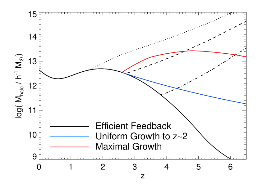
Figure 13 shows the bias and correlation length predicted by this approach, an extension of the model (Equation 8) we have considered at $z\lesssim 2$. Figure 14 also shows the typical host halo mass corresponding to the predicted clustering as a function of redshift (for our adopted cosmology); in this simple extension of the $z\lesssim 3$ case, the observed decline in the QLF $L_{\ast}$ traces a decline in the characteristic (although not most massive) quasar-hosting halo mass.

Figure 13.— Using the model in Figures 1 & 6 to predict the observable clustering of quasars at high redshifts $z\gtrsim 3$. Observed clustering is shown (points) as in Figure 1. Different lines show the effect of different observed-frame $i$-band flux limits, as labeled (note $i=20.2$ corresponds to the SDSS DR3 completeness limit; Richards et al., 2006a). Left panels assume efficient feedback at high redshifts; i.e. that BH growth “shuts down” after each quasar episode. Center panels assume all $z>2$ BHs grow with the observed QLF to the characteristic peak luminosities at $z\sim 2$, then shut down (“inefficient feedback”). Right panels assume quasar growth tracks host halo growth, even after a quasar episode, until $z=2$ (“maximal growth”). Future observations at $z\sim 4$ with moderately improved flux limits $m_{i}<22$ should be able to break the degeneracies between these models.

Figure 14.— Characteristic inferred quasar-hosting halo mass corresponding to the model clustering as a function of redshift shown in Figure 13, for our adopted cosmology. Dotted, dashed, and dot-dashed lines are for the appropriate flux limits as in Figure 13. The black, blue, and red lines show the left, center, and right models (“efficient feedback”, growth to typical $z\sim 2$ quasars, and “maximal” growth, respectively) from Figure 13 with effectively infinitely deep flux limits ($i<30$); all are identical below $z\sim 2.6$.

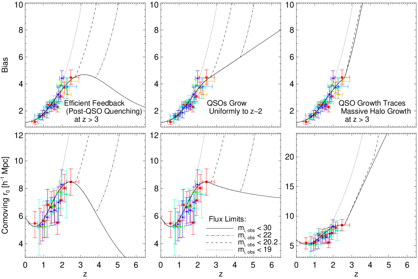
However, at high redshifts, flux limits may severely bias clustering measurements. Although at $L<L_{\ast}$, quasar clustering does not strongly depend on the quasar luminosity (see § 3), implying a well-defined characteristic active mass which we can adopt (see also Lidz et al., 2006), this is not necessarily true for $L>L_{\ast}$. In fact, Figure 3 shows (and observations may begin to see, e.g. Porciani & Norberg, 2006) a steepening of bias versus luminosity at $L>L_{\ast}$, reflecting the uniformly high observed quasar Eddington ratios (Vestergaard, 2004; McLure & Dunlop, 2004; Kollmeier et al., 2005) at high luminosities, which imply the bright end of the QLF ($L\gg L_{\ast}$) becomes predominantly a sequence in active BH mass. To the extent that BH mass traces host mass, then, these systems reside in more massive hosts and will be more strongly biased.

In order to estimate how this will change the observed clustering, we roughly approximate this effect as follows. For a given flux limit at a given redshift there is a reasonably well-defined survey depth, to a minimum luminosity $L_{\rm min}$. If this is sufficiently deep to resolve the QLF “break,” i.e. $L_{\rm min}<L_{\ast}$, then the weak observed dependence of clustering on luminosity means the observed clustering will trace that characteristic of $\sim L_{\ast}$ quasars – corresponding to characteristic $M_{\rm BH}$ active BHs and $M_{\rm gal}\approx M_{\rm BH}/\mu$ hosts (our fiducial model, and the case for all observations plotted in Figure 13). However, if the flux limit or redshift is sufficiently high such that $L_{\rm min}>L_{\ast}$, then the survey will not sample these characteristic host masses. In this case, we consider the bias as a function of luminosity plotted in Figure 3 from the models of Hopkins et al. (2006b); Lidz et al. (2006), evaluated at $L_{\rm min}$ at the given redshift. Qualitatively, for the nearly constant Eddington ratios observed at $L>L_{\ast}$, $L\propto M_{\rm BH}\propto M_{\rm gal}$, we expect $L_{\rm min}>L_{\ast}$ to correspond to an approximate minimum observed host mass, $M_{\rm min}\sim M_{\rm gal}(L_{\ast})\times(L_{\rm min}/L_{\ast})\sim M_{\rm Edd}(L_{\rm min})/\mu$. Since the QLF slope is steep at $L>L_{\ast}$, objects near $L_{\rm min}$ or $M_{\rm min}$ will dominate the observed sample, and so this amounts to calculating the clustering for this mass, instead of $M_{\rm gal}(L_{\ast})$, at the given redshift. We caution that this is a rough approximation to more realistic selection effects, but should give us some idea how flux limits will bias the observed clustering.

We consider several representative flux limits, in observed-frame $i$-band, typical of optical quasar surveys (e.g. the SDSS), in addition to the case with effectively infinite depth ($m_{i}<30$). We calculate $L_{\ast}$ at the appropriate rest-frame wavelengths as a function of redshift using the fits to $L_{\ast}$ from Hopkins et al. (2007b), spanning $z\sim 0-6$ and spanning the relevant rest-frame wavelength intervals. At the limits of most current optical surveys, $m_{i}<20.2$, the QLF break $L_{\ast}$ is only marginally resolved at $z\sim 2-3$, and so above this redshift surveys are systematically biased to more massive $L>L_{\ast}$ BHs and higher clustering amplitudes. However, a relatively modest improvement in depth to $m_{i}<22$ would allow unbiased clustering estimates to be extended to $z\sim 4$.

We have so far assumed BHs effectively “shut down” after their quasar epoch – i.e. “efficient feedback” even at high redshifts. Although the various observations discussed above (Eddington ratio distributions, quasar host measurements, HOD models, black hole mass functions, and our clustering comparison) demand this be true at $z\lesssim 2-3$, there are no such constraints at $z\gtrsim 3$. In other words, it is possible that the increase in the QLF from $z\sim 6$ to $z\sim 3$ traces the growth of the same populations of BHs, not the subsequent triggering and “shutdown” of different populations. If BHs at $z\sim 6$ continue to grow to $z\sim 2-3$ before “shutting down,” they must live in more massive $z=0$ host galaxies (to preserve the tight observed BH-host mass relation), and thus should have stronger clustering amplitudes. We therefore consider two representative simple models which bracket the range of possibilities for this growth and present simple tests for future clustering measurements to break the degeneracy between these models.

First, we assume that quasars grow with the QLF to $z\sim 2$ before “shutting down” (i.e. “inefficient feedback”). In such a case, $z\sim 6$ quasars grow either continuously or episodically with their host systems until the epoch where “downsizing” begins, and the QLF at all redshifts $z>2$ represents the same systems building up hierarchically. The $z=0$ relic masses (and therefore $z=0$ characteristic host masses, from which we calculate the “parent” halo clustering as a function of redshift) are then the same at all $z\geq 2$. This is also equivalent to a “pure density evolution” model for the high redshift QLF, as in Fan et al. (2001), in which the QLF break luminosity $L_{\ast}$ remains constant above $z\sim 2-3$ while the number density/normalization uniformly declines. Such a model is marginally disfavored by current measurements (Hopkins et al., 2007b), but constraints on $L_{\ast}$ at high redshifts are sufficiently weak that it remains a possibility.

The clustering as a function of redshift in this model behaves very differently from the previous model at high redshifts. If objects cannot grow after their quasar epoch even at high redshifts, then the subsequent decline of the QLF $L_{\ast}$ traces a decline in characteristic active masses, and the bias of active systems “turns over”; however, if all grow to the characteristic $L_{\ast}$ at $z\sim 2$, then these high redshift systems all represent similar $z=0$ masses by the time they “shut down,” and must be increasingly biased at higher redshifts.

Next, we consider a “maximal” growth model, in which we assume not only that the buildup of the QLF represents the continued growth of BHs until $z\sim 2$, but also that this growth proportionally tracks the typical growth of dark matter halos over this redshift range. We very crudely estimate the “typical growth” with the growth of an average high-redshift quasar “host” halo. Based on their space density and BH mass, Fan et al. (2001, 2003) estimate that typical $z\sim 5-6$ SDSS quasars represent $\sim 6\sigma$ overdensities. We therefore assume that quasars at a given redshift $z>2$, with a typical $L_{\ast}$ and corresponding $M_{\rm BH}$ at that redshift, will grow by the same proportional amount as a halo which represents a $6\sigma$ fluctuation (characteristic of halos hosting observed $z\sim 6$ quasars, Y. Li et al., 2006) from the observed redshift to $z=2$, after which growth “shuts down.” This then yields the $z=0$ BH mass, corresponding host mass, and evolved clustering. Note that, although similar, this is not the same as assuming quasars track $6\sigma$ overdensities at $z>2$, because to the extent that the QLF $L_{\ast}$ does not grow by the same proportionality, this model effectively allows “new” or different BHs/host halos to dominate the QLF at different redshifts. It simply mandates that they all grow at this rapid rate. For example, an observed $z\sim 6$ BH of $\sim 10^{8}\,M_{\sun}$ is assumed to reach a mass of $2\times 10^{9}\,M_{\sun}$ at $z=2$ (and then shuts down, so that this is also the mass at $z=0$), and a $\sim 10^{8}\,M_{\sun}$ observed quasar at $z=4$ will grow to $\sim 5\times 10^{8}\,M_{\sun}$. The choice of rate is arbitrary, we choose it as a reasonable upper limit. In any case, the predicted evolution of the bias as a function of redshift is extremely steep, so the exact values will be very sensitive to the growth model and adopted cosmology. The point we wish to illustrate is that this model generically predicts a steep bias evolution at $z>2$, which regardless of the details will be distinguishable if future quasar clustering measurements at $z=3-4$ can be extended to a depth of $m_{i}<22$.

Note that extending the depth of quasar surveys to $m_{i}<22$ will move further down the QLF and increase the density of quasars observed, meaning a smaller survey can be used to constrain the clustering to comparable accuracy as the SDSS or 2dF. Using the Hopkins et al. (2007b) QLF to estimate the relevant space density of quasars above the flux limit as a function of redshift and assuming the errors in clustering amplitude relative to those in Croom et al. (2005) scale as $N_{\rm qso}^{-1/2}$, we estimate that for the redshift interval $3.5<z<4.5$ ($3.75<z<4.25$) a field size of $\sim 25\,{\rm deg}^{2}$ ($50\,{\rm deg}^{2}$) would be sufficient to distinguish between the first two models (efficient high-redshift feedback and all high-redshift quasars growing to $z\sim 2$ luminosities) at $\sim 2.5-3\,\sigma$. The last model (“maximal evolution”) predicts an even more extreme departure in clustering properties, and could be distinguished or ruled out at $\sim 2.5-3\,\sigma$ by clustering observations from $2.75<z<3.25$ in just a $\sim 8-15\,{\rm deg}^{2}$ field.

7. Discussion/Conclusions

We compare the clustering of quasars and different galaxy populations as a function of morphology, mass, luminosity, and redshift, and demonstrate that these comparisons can be used to robustly rule out several classes of models for quasar triggering and the association between quasar and galaxy growth. In each case, the observations favor a model which associates quasars with the “formation event” of ellipticals, a strong prediction of theoretical models which argue that major, gas-rich mergers form ellipticals and trigger quasar activity (Hopkins et al., 2006b).

The predicted bias as a function of mass/luminosity for systems which once hosted quasars agrees well at all masses and luminosities with that observed for early-type populations. In other words, the clustering of an $M_{\rm gal}$ elliptical galaxy is exactly what we would expect if these galaxies, which typically contain $M_{\rm BH}=\mu\,M_{\rm gal}$ ($\mu\sim 0.001$ Magorrian et al., 1998; Marconi & Hunt, 2003; Häring & Rix, 2004) BHs, represented the dominant “hosts” of the quasar population for a brief period, setting $L_{\ast}$ at that redshift with an Eddington-limited $L_{\ast}=L_{\rm Edd}(M_{\rm BH})$ “epoch” of activity. In the most basic sense, this is a confirmation that ellipticals today were indeed the host population of high-redshift quasars (see also Porciani et al., 2004; Croom et al., 2005), with the appropriate corresponding BH masses. This should not be surprising, since the Soltan (1982) argument demonstrates that most BH mass must have been accumulated in bright, near-Eddington “quasar” epochs, and the tightness of the local BH-host mass relation (and similar BH mass-host property relations, see Novak et al., 2006) argues that BH growth must be tightly coupled to the host properties. However, there are additional non-trivial implications.

First, this implies that there really is a characteristic host and BH mass “active” at a given epoch, traced by the QLF $L_{\ast}$. This is an important prediction of certain theoretical models for quasar lightcurves (Hopkins et al., 2005c, d), and supported by other lines of observation above. Furthermore, this implies that the formation “epoch” for BHs of a given mass must be relatively short in time, as continually adding BHs of a given mass (at lower Eddington ratio or in radiatively inefficient states) to the population would dilute the agreement in Figure 1. Quasars are active in characteristically different parent halo populations at different redshifts – i.e. most systems cannot undergo multiple separate periods of quasar activity, at least at $z\lesssim 2$. We find further support for this by considering observed quasar clustering as a function of luminosity, which favors the predictions of Lidz et al. (2006), namely a relatively weak trend of bias as a function of luminosity. In fact, the combination of quasar clustering measurements as a function of luminosity and redshift supports at high significance previous suggestions of little or no luminosity dependence (e.g., Adelberger & Steidel, 2005a; Myers et al., 2006, 2007a), and is inconsistent with the predictions of simplified “light bulb” or exponential quasar light curve models (e.g., Kauffmann & Haehnelt, 2002; Wyithe & Loeb, 2003) at $>4-5\,\sigma$.

This relates to a subtle but important distinction: this implies that the halos of the dominant population of $M_{\rm gal}$ ellipticals are the same halos as those which hosted the corresponding quasar activity. A significant fraction of the $M_{\rm gal}$ early-type population cannot form from later collapsing halos, as this both requires the buildup of BHs of the same mass at a different time, ruled out by the observations above, and would dilute the clustering agreement.

Second, the clustering of late-type galaxies at a given luminosity or mass does not agree with the evolved clustering of quasars. This argues that it is specifically the progenitors of early-type galaxies which hosted quasars. Although this is not surprising, given that observations find it is specifically bulge mass/velocity dispersion which correlates with BH mass (Gebhardt et al., 2000; Ferrarese & Merritt, 2000; McLure & Dunlop, 2002; Häring & Rix, 2004), there still exist classes of models which would generically associate BH formation with galaxy formation, star formation, or halo virialization. Our comparison of observations rules out these scenarios.

We further invert our comparisons to predict quasar clustering as a function of redshift, and compare this with the observed clustering of red and blue galaxies at each redshift. Quasars do not trace a uniform/constant population with redshift – i.e. they are not cosmologically long-lived, as has been noted in many previous clustering studies (see Porciani et al., 2004; Martini, 2004; Croom et al., 2005). Further, quasars do not trace the clustering of “established” red or blue galaxy populations. This rules out models in which quasars are associated with cyclic (e.g., Ciotti & Ostriker, 2001; Binney, 2004) or radio “heating” modes over a Hubble time in red galaxies, as well as (at least the most straightforward implementations of) models which generically associate quasars with star formation (e.g., Granato et al., 2004) or disk instabilities in high-redshift, gas-rich disk systems (e.g., Kauffmann & Haehnelt, 2000).

Note, however, that this does not rule out the presence of these accretion modes at low luminosities and/or low redshifts. Many of the observations discussed above limit bright, high Eddington ratio quasar activity to a single, short-lived epoch. Long-lived accretion in a “radio-mode” is believed to be associated with particularly low Eddington ratio activity (Ho, 2002; White et al., 2006), perhaps an entirely different accretion state (Narayan & Yi, 1995; Marchesini et al., 2004; Jester, 2005; Pellegrini, 2005; Koerding et al., 2006), and not typical $L_{\ast}$ QLF activity. Models which invoke “radio mode” type accretion at low Eddington ratios in quasar “relics” (e.g., Croton et al., 2006; De Lucia et al., 2006) are therefore completely consistent with the clustering arguments herein. Other observations of black hole mass functions and quasar Eddington ratios (Yu & Tremaine, 2002; McLure & Dunlop, 2004; Kollmeier et al., 2005) also rule out “cyclic” models, insofar as they attempt to explain more luminous $\sim L_{\ast}$ quasar activity. However, theoretical models of stochastic, feedback-regulated accretion in gas-rich systems (Hopkins & Hernquist, 2006) predict that these fueling modes dominate at low redshift and at typical “Seyfert” luminosities at higher redshifts, even where mergers (Hopkins et al., 2006c, 2007a) may dominate the bright $\sim L_{\ast}$ quasar population. We demonstrate that the luminosities at which these “Seyfert” accretion modes may dominate are sufficiently low that they have no effect on our results. However, we make predictions for future measurements of clustering as a function of luminosity at moderate redshifts, which may be able to detect such changes in the characteristic host population and fueling mechanisms through the cross-correlation of galaxies and faint, X-ray selected AGN in deep fields at $z\sim 1$.

It is also important to distinguish the processes which may be associated with the initial formation of ellipticals from their subsequent evolution. Once morphologically transformed by a gas-rich merger, for example, mass can be moved “up” the red sequence (galaxies increased in mass) by gas-poor mergers, which will involve neither star formation nor quasar activity, but it cannot be added to the red sequence in this manner. As noted above, low-luminosity AGN or “radio mode” activity, or halo shock “quenching” may be of critical importance to suppressing cooling flows and further accretion in massive ellipticals. However, these do not appear to be associated with the initial formation of an elliptical or triggering of traditional, bright, high-redshift quasars.

It is interesting that, at all redshifts, quasars clustering is observed to be intermediate between blue and red galaxy clustering. To the extent that halos grow monotonically with time, intermediate clustering may imply intermediate halo mass and therefore, perhaps, an intermediate evolutionary stage – i.e. quasars are representative of an evolutionary state “between” blue and red galaxies. This is predicted in many theoretical models (Granato et al., 2004; Scannapieco & Oh, 2004; Springel et al., 2005a; Monaco & Fontanot, 2005; Hopkins et al., 2006b, 2007a), which posit that quasar feedback, or a merger-triggered quasar phase, is associated with (regardless of whether or not it directly causes) the formation of ellipticals and “transition” of galaxies to the red sequence. Quasars do appear to cluster similarly to likely “merger” populations (close pairs, post-starburst/E+A galaxies, and sub-millimeter galaxies) at both low ($z\lesssim 0.3$) and high ($z\sim 2-3$) redshifts, but more detailed measurements of these populations are needed. We confirm the finding from previous studies (Porciani et al., 2004; Croom et al., 2005; Porciani & Norberg, 2006; Myers et al., 2006, 2007a) that quasar clustering is consistent with a constant halo mass $\sim 4\times 10^{12}\,h^{-1}\,M_{\sun}$; interestingly, similar to the characteristic mass of small galaxy groups (at least at low redshift) in which galaxy-galaxy major mergers are expected to be most efficient. Further theoretical investigation of this, and the possibility that it may manifest in an excess of quasar clustering on small scales (e.g., Hennawi et al., 2006, but see also Myers et al. 2007b), are important subjects for future work. We calculate the implied time delay between the star-forming/LBG “phase” of evolution, quasar phase, and red galaxy phase, from the evolved clustering of halos of a given initial mass. Although this is just a “toy” model of self-similar halo evolution, suggestively, the time from quasar epoch to “red galaxy” epoch corresponds reasonably at all redshifts with the delay expected for stellar populations to redden to typical red galaxy colors after the termination or “shutdown” of star formation. We caution, however, that the systematic uncertainties in measurements of these clustering strengths (especially at high redshifts) remain a concern, and future studies which compare uniformly selected galaxy and quasar populations across a wide range of redshifts adopting consistent measurement methods are needed to make these conclusions robust.

We explore this further by considering the age of BHs (i.e. the time since the mean “formation” or quasar epoch for BHs of a given relic mass) as a function of mass, and comparing this with the age of their hosts. The mean stellar age (and dispersion in ages) of early-type BH hosts agrees well at all masses, implying that quasars are associated with the formation epoch of early-type galaxies. Specifically, these are light-weighted or single-burst ages of red galaxies, which tend to reflect the last significant epoch of star formation – i.e. quasars are associated with the last significant epoch (or potentially the termination) of star formation in elliptical hosts. This association can be used to accurately predict quasar clustering as a function of redshift in a purely empirical manner, without any assumptions about quasar light curves, lifetimes, or Eddington ratios.

A similar association does not hold for disk-dominated systems hosting BHs; i.e. again demonstrating that BH growth and quasar activity do not generically trace star formation. Likewise, such an association does not hold for dark matter halos, meaning that quasars do not generically trace halo formation/assembly (even accounting for the halo downsizing effects seen in Neistein et al., 2006). They also do not generically trace the crossing of host halos of the critical shock “quenching” mass in Birnboim & Dekel (2003); Kereš et al. (2005); Dekel & Birnboim (2006). Although our comparisons are consistent with the possibility that this halo mass does “quench” gas accretion (and thus quasar activity will not generally occur at higher masses), there must be a mechanism which can trigger quasars before they cross this threshold.

We emphasize that this does not imply that most of the stars in spheroids form in such a short-lived burst contemporaneous with their quasar epoch. Direct calculation of the inferred stellar population ages from line index and SED fitting (following Trager et al., 2000) for realistic star formation histories from the semi-analytic models of Somerville et al. (2001) and hydrodynamical merger simulations of Robertson et al. (2006b) suggests that the ages inferred for present early-type galaxies indeed reflect the epoch of the termination of star formation, even when $\gtrsim 95\%$ of stars are formed over a much longer timescale at significantly earlier times (in these cases, in quiescent star formation in disks). Indeed, most models (e.g., Hopkins et al., 2006e; Croton et al., 2006; De Lucia et al., 2006) predict that only a small fraction of stars in ellipticals were formed in merger-induced starbursts. This, combined with the lack of a general correlation between star formation in disks and quasar activity, supports the hypothesis that quasars trace the end of star formation in present spheroids, as predicted by models which associate quasar activity with mergers (or other mechanisms) that rapidly exhaust gas and transform (assemble) disks into spheroids.

Finally, we extend these empirical predictions of quasar clustering to high redshift, and show that the $z>2-3$ clustering of quasars is dramatically different depending on whether or not feedback is efficient at high redshift (i.e. whether or not $z>2$ quasars “shut down” after their quasar episode, as observations show they do at $z<2$). Present observations cannot distinguish these possibilities, but future quasar samples at $z\sim 3-4$ with flux limits $m_{i}\lesssim 22$ should be able to break the degeneracies.

Although there are non-negligible uncertainties in these conversions to characteristic host masses or luminosities, a number of different lines of evidence support their robustness. The conversion to a characteristic BH mass (and the lack of evolution to $z=0$) is determined by direct Eddington ratio observations (Heckman et al., 2004; Vestergaard, 2004; McLure & Dunlop, 2004; Kollmeier et al., 2005; Hopkins, Hernquist, & Narayan, 2005) and observed cosmic background constraints (Elvis et al., 2002; Ueda et al., 2003; Cao, 2005). If we instead adopt the simplest empirically inferred models of quasar lightcurves from matching the QLF and local BH mass function (Yu & Tremaine, 2002; Marconi et al., 2004; Shankar et al., 2004; Hopkins et al., 2007b), we come to an identical conclusion. Likewise for more sophisticated models which incorporate effects of different accretion states and compare radio, X-ray, and optical QLFs (Merloni, 2004), and theoretical models of quasar light curves from numerical hydrodynamic simulations of galaxy mergers which dynamically incorporate BH growth and feedback (Hopkins et al., 2006b). Whether we adopt the observed BH-host mass/luminosity relations, or those from simulations (Di Matteo et al., 2005; Robertson et al., 2006a; Hopkins et al., 2005a, b, c), we obtain an identical result. Adopting just the BH-host mass relation, and using the time since the quasar epoch to determine the observed $M/L$ (i.e. assuming this represents a stellar age and using the population synthesis models of Bruzual & Charlot (2003) to predict $M/L$ in a given band) also does not change this comparison.

Finally, direct construction of halo occupation (HOD) models from observed quasar clustering (Porciani et al., 2004; Porciani & Norberg, 2006; Adelberger & Steidel, 2005b; Croom et al., 2005) leads to the same conclusions regarding the luminosity $L_{\ast}$ reflecting the evolving characteristic mass of active quasars, their weak subsequent BH growth, and host properties at $z=0$. In other words, our uncertainties in this approach are most likely dominated by the substantial measurement errors in the bias $b(z)$ of quasar and galaxy populations, not by the systematics in our methodology. As such, future improved measurements of quasar clustering and bias at high redshifts, particularly as a function of luminosity (e.g. using the proximity effect; Faucher-Giguere et al. 2006), as well as improved galaxy clustering measurements which can resolve the clustering as a function of mass or luminosity at $z\gtrsim 1$, will strengthen the constraints herein and continue to inform models for quasar fueling and their associations with spheroid formation.

References

- Adelberger & Steidel (2005a) Adelberger, K. L., & Steidel, C. C. 2005a, ApJ, 630, 50
- Adelberger & Steidel (2005b) Adelberger, K. L., & Steidel, C. C. 2005b, ApJ, 627, L1
- Adelberger et al. (2005) Adelberger, K. L., Steidel, C. C., Pettini, M., Shapley, A. E., Reddy, N. A., & Erb, D. K. 2005, ApJ, 619, 697
- Allen et al. (2005) Allen, P. D., Moustakas, L. A., Dalton, G., MacDonald, E., Blake, C., Clewley, L., Heymans, C., & Wegner, G. 2005, MNRAS, 360, 1244
- Aller & Richstone (2002) Aller, M. C., & Richstone, D. 2002, AJ, 124, 3035
- Barnes & Hernquist (1991) Barnes, J. E. & Hernquist, L. 1991, ApJ, 370, L65
- Barnes & Hernquist (1996) Barnes, J. E. & Hernquist, L. 1996, ApJ, 471, 115
- Baugh et al. (2005) Baugh, C. M., Lacey, C. G., Frenk, C. S., Granato, G. L., Silva, L., Bressan, A., Benson, A. J., & Cole, S. 2005, MNRAS, 356, 1191
- Bell et al. (2000) Bell, E. F., Barnaby, D., Bower, R. G., de Jong, R. S., Harper, D. A., Hereld, M., Loewenstein, R. F., & Rauscher, B. J. 2000, MNRAS, 312, 470
- Bell & de Jong (2000) Bell, E. F., & de Jong, R. S. 2000, MNRAS, 312, 497
- Bell et al. (2003) Bell, E. F., McIntosh, D. H., Katz, N., & Weinberg, M. D. 2003, ApJS, 149, 289
- Bernardi et al. (2005) Bernardi, M., Sheth, R. K., Nichol, R. C., Schneider, D. P., & Brinkmann, J. 2005, AJ, 129, 61
- Bernardi et al. (2006) Bernardi, M., Nichol, R. C., Sheth, R. K., Miller, C. J., & Brinkmann, J. 2006, AJ, 131, 1288
- Best et al. (2005) Best, P. N., Kauffmann, G., Heckman, T. M., Brinchmann, J., Charlot, S., Ivezić, Ž., & White, S. D. M. 2005, MNRAS, 362, 25
- Binney (2004) Binney, J. 2004, MNRAS, 347, 1093
- Birnboim & Dekel (2003) Birnboim, Y., & Dekel, A. 2003, MNRAS, 345, 349
- Blain et al. (2004) Blain, A. W., Chapman, S. C., Smail, I., & Ivison, R. 2004, ApJ, 611, 725
- Blake et al. (2004) Blake, C., et al. 2004, MNRAS, 355, 713
- Boselli et al. (2001) Boselli, A., Gavazzi, G., Donas, J., & Scodeggio, M. 2001, AJ, 121, 753
- Bower et al. (2006) Bower, R. G., Benson, A. J., Malbon, R., Helly, J. C., Frenk, C. S., Baugh, C. M., Cole, S., & Lacey, C. G. 2006, MNRAS, 370, 645
- Boyle et al. (2000) Boyle, B. J., Shanks, T., Croom, S. M., Smith, R. J., Miller, L., Loaring, N., & Heymans, C. 2000, MNRAS, 317, 1014
- Brinchmann et al. (2004) Brinchmann, J., Charlot, S., White, S. D. M., Tremonti, C., Kauffmann, G., Heckman, T., & Brinkmann, J. 2004, MNRAS, 351, 1151
- Brown et al. (2001) Brown, M. J. I., Boyle, B. J., & Webster, R. L. 2001, AJ, 122, 26
- Brown et al. (2003) Brown, M. J. I., Dey, A., Jannuzi, B. T., Lauer, T. R., Tiede, G. P., & Mikles, V. J. 2003, ApJ, 597, 225
- Brown et al. (2005) Brown, M. J. I., Jannuzi, B. T., Dey, A., & Tiede, G. P. 2005, ApJ, 621, 41
- Bruzual & Charlot (2003) Bruzual, G., & Charlot, S. 2003, MNRAS, 344, 1000
- Caldwell et al. (2003) Caldwell, N., Rose, J. A., & Concannon, K. D. 2003, AJ, 125, 2891
- Cao (2005) Cao, X. 2005, ApJ, 631, L101
- Cattaneo et al. (2006) Cattaneo, A., Dekel, A., Devriendt, J., Guiderdoni, B., & Blaizot, J. 2006, MNRAS, 370, 1651
- Chakrabarti et al. (2006) Chakrabarti, S., Fenner, Y., Hernquist, L., Cox, T. J., & Hopkins, P. F. 2006, ApJ, in press [astro-ph/0610860]
- Ciotti & Ostriker (2001) Ciotti, L., & Ostriker, J. P. 2001, ApJ, 551, 131
- Clemens et al. (2006) Clemens, M. S., Bressan, A., Nikolic, B., Alexander, P., Annibali, F., & Rampazzo, R. 2006, MNRAS, 370, 702
- Coil et al. (2004) Coil, A. L., et al. 2004, ApJ, 609, 525
- Coil et al. (2006a) Coil, A. L., et al. 2006a, ApJ, 638, 668
- Coil et al. (2006b) Coil, A. L., Hennawi, J. F., Newman, J. A., Cooper, M. C., & Davis, M. 2006b, ApJ, in press [astro-ph/0607454]
- Coil et al. (2006c) Coil, A. L., Newman, J. A., Cooper, M. C., Davis, M., Faber, S. M., Koo, D. C., & Willmer, C. N. A. 2006c, ApJ, 644, 671
- Collobert et al. (2006) Collobert, M., Sarzi, M., Davies, R. L., Kuntschner, H., & Colless, M. 2006, MNRAS, 370, 1213
- Constantin & Vogeley (2006) Constantin, A., & Vogeley, M. S. 2006, ApJ, 650, 727
- Cox et al. (2006) Cox, T. J., Dutta, S. N., Di Matteo, T., Hernquist, L., Hopkins, P. F., Robertson, B., & Springel, V. 2006, ApJ, 650, 791
- Croom et al. (2001) Croom, S. M., Shanks, T., Boyle, B. J., Smith, R. J., Miller, L., Loaring, N. S., & Hoyle, F. 2001, MNRAS, 325, 483
- Croom et al. (2002) Croom, S. M., Boyle, B. J., Loaring, N. S., Miller, L., Outram, P. J., Shanks, T., & Smith, R. J. 2002, MNRAS, 335, 459
- Croom et al. (2004) Croom, S. M., Smith, R. J., Boyle, B. J., Shanks, T., Miller, L., Outram, P. J., & Loaring, N. S. 2004, MNRAS, 349, 1397
- Croom et al. (2005) Croom, S. M., et al. 2005, MNRAS, 356, 415
- Croton et al. (2006) Croton, D. J., et al. 2006, MNRAS, 365, 11
- Croton et al. (2007) Croton, D. J., Gao, L., & White, S. D. M. 2007, MNRAS, 374, 1303
- Dekel & Birnboim (2006) Dekel, A., & Birnboim, Y. 2006, MNRAS, 368, 2
- De Lucia et al. (2006) De Lucia, G. & Blaizot, J. 2006, MNRAS, in press [astro-ph/0606519]
- Di Matteo et al. (2005) Di Matteo, T., Springel, V., & Hernquist, L. 2005, Nature, 433, 604
- di Serego Alighieri et al. (2006) di Serego Alighieri, S., Lanzoni, B., & Jørgensen, I. 2006, ApJ, 647, L99
- Dong & De Robertis (2006) Dong, X. Y., & De Robertis, M. M. 2006, AJ, 131, 1236
- Eisenstein & Hu (1999) Eisenstein, D. J., & Hu, W. 1999, ApJ, 511, 5
- Elvis et al. (2002) Elvis, M., Risaliti, G., & Zamorani, G. 2002, ApJ, 565, L75
- Fan et al. (2001) Fan, X., et al. 2001, AJ, 121, 54
- Fan et al. (2003) Fan, X., et al. 2003, AJ, 125, 1649
- Faucher-Giguere et al. (2006) Faucher-Giguere, C.-A. et al. 2006, ApJ, submitted
- Ferrarese & Merritt (2000) Ferrarese, L. & Merritt, D. 2000, ApJ, 539, L9
- Firth et al. (2002) Firth, A. E., et al. 2002, MNRAS, 332, 617
- Fry (1996) Fry, J. N. 1996, ApJ, 461, L65
- Fukugita et al. (1998) Fukugita, M., Hogan, C. J., & Peebles, P. J. E. 1998, ApJ, 503, 518
- Furlanetto & Kamionkowski (2006) Furlanetto, S. R., & Kamionkowski, M. 2006, MNRAS, 366, 529
- Gallazzi et al. (2005) Gallazzi, A., Charlot, S., Brinchmann, J., White, S. D. M., & Tremonti, C. A. 2005, MNRAS, 362, 41
- Gallazzi et al. (2006) Gallazzi, A., Charlot, S., Brinchmann, J., & White, S. D. M. 2006, MNRAS, 370, 1106
- Gao & White (2006) Gao, L., & White, S. D. M. 2006, MNRAS, in press [astro-ph/0611921]
- Gavazzi et al. (2002) Gavazzi, G., Bonfanti, C., Sanvito, G., Boselli, A., & Scodeggio, M. 2002, ApJ, 576, 135
- Gebhardt et al. (2000) Gebhardt, K., Bender, R., Bower, G. et al. 2000, ApJ, 539, L13
- Giavalisco & Dickinson (2001) Giavalisco, M., & Dickinson, M. 2001, ApJ, 550, 177
- Goto (2005) Goto, T. 2005, MNRAS, 357, 937
- Graham et al. (2001) Graham, A. W., Erwin, P., Caon, N., & Trujillo, I. 2001, ApJ, 563, L11
- Granato et al. (2004) Granato, G. L., De Zotti, G., Silva, L., Bressan, A., & Danese, L. 2004, ApJ, 600, 580
- Grazian et al. (2004) Grazian, A., Negrello, M., Moscardini, L., Cristiani, S., Haehnelt, M. G., Matarrese, S., Omizzolo, A., & Vanzella, E. 2004, AJ, 127, 592
- Grazian et al. (2006) Grazian, A., et al. 2006, A&A, 453, 507
- Harker et al. (2006) Harker, J. J., Schiavon, R. P., Weiner, B. J., & Faber, S. M. 2006, ApJ, 647, L103
- G. Harker et al. (2006) Harker, G., Cole, S., Helly, J., Frenk, C., & Jenkins, A. 2006, MNRAS, 367, 1039
- Häring & Rix (2004) Häring, N., & Rix, H.-W. 2004, ApJ, 604, L89
- Hasinger et al. (2005) Hasinger, G., Miyaji, T., & Schmidt, M. 2005, A&A, 441, 417
- Heckman et al. (2004) Heckman, T. M., Kauffmann, G., Brinchmann, J., Charlot, S., Tremonti, C., & White, S. D. M. 2004, ApJ, 613, 109
- Hennawi et al. (2006) Hennawi, J. F., et al. 2006, AJ, 131, 1
- Ho (2002) Ho, L. C. 2002, ApJ, 564, 120
- Hopkins & Beacom (2006) Hopkins, A. M., & Beacom, J. F. 2006, ApJ, 651, 142
- Hopkins et al. (2005a) Hopkins, P. F., Hernquist, L., Martini, P., Cox, T. J., Robertson, B., Di Matteo, T., & Springel, V. 2005a, ApJ, 625, L71
- Hopkins et al. (2005b) Hopkins, P. F., Hernquist, L., Cox, T. J., Robertson, B., Di Matteo, T., Martini, P., & Springel, V. 2005b, ApJ, 630, 705
- Hopkins et al. (2005c) Hopkins, P. F., Hernquist, L., Cox, T. J., Robertson, B., Di Matteo, T., & Springel, V. 2005c, ApJ, 630, 716
- Hopkins et al. (2005d) Hopkins, P. F., Hernquist, L., Cox, T. J., Robertson, B., Di Matteo, T., & Springel, V. 2005d, ApJ, 632, 81
- Hopkins et al. (2006a) Hopkins, P. F., Hernquist, L., Cox, T. J., Robertson, B., Di Matteo, T., & Springel, V. 2006a, ApJ, 639, 700
- Hopkins et al. (2006b) Hopkins, P. F., Hernquist, L., Cox, T. J., Robertson, B., Di Matteo, T., & Springel, V. 2006b, ApJS, 163, 1
- Hopkins et al. (2006c) Hopkins, P. F., Hernquist, L., Cox, T. J., Robertson, B., & Springel, V. 2006c, ApJS, 163, 50
- Hopkins et al. (2006d) Hopkins, P. F., Robertson, B., Krause, E., Hernquist, L., & Cox, T. J. 2006d, ApJ, 652, 107
- Hopkins et al. (2006e) Hopkins, P. F., Somerville, R. S., Hernquist, L., Cox, T. J., Robertson, B., & Li, Y. 2006e, ApJ, 652, 864
- Hopkins et al. (2007a) Hopkins, P. F., Bundy, K., Hernquist, L., & Ellis, R. S. 2007a, ApJ, 659, 976
- Hopkins et al. (2007b) Hopkins, P. F., Richards, G. T., & Hernquist, L. 2007b, ApJ, 654, 731
- Hopkins & Hernquist (2006) Hopkins, P. F., & Hernquist, L. 2006, ApJS, 166, 1
- Hopkins, Hernquist, & Narayan (2005) Hopkins, P. F., Hernquist, L., Narayan, R. 2005, ApJ, 643, 641
- Hunt et al. (2004) Hunt, L. K., Pierini, D., & Giovanardi, C. 2004, A&A, 414, 905
- Infante et al. (2002) Infante, L., et al. 2002, ApJ, 567, 155
- Jansen et al. (2000) Jansen, R. A., Fabricant, D., Franx, M., & Caldwell, N. 2000, ApJS, 126, 331
- Jester (2005) Jester, S. 2005, ApJ, 625, 667
- Jørgensen (1999) Jørgensen, I. 1999, MNRAS, 306, 607
- Kauffmann & Haehnelt (2000) Kauffmann, G. & Haehnelt, M. G. 2000, MNRAS, 311, 576
- Kauffmann & Haehnelt (2002) Kauffmann, G., & Haehnelt, M. G. 2002, MNRAS, 332, 529
- Kauffmann et al. (2003a) Kauffmann, G., et al. 2003a, MNRAS, 341, 54
- Kauffmann et al. (2003b) Kauffmann, G., et al. 2003b, MNRAS, 346, 1055
- Kereš et al. (2005) Kereš, D., Katz, N., Weinberg, D. H., & Davé, R. 2005, MNRAS, 363, 2
- Koerding et al. (2006) Körding, E. G., Jester, S., & Fender, R. 2006, MNRAS, 372, 1366
- Kollmeier et al. (2005) Kollmeier, J. A., et al. 2006, ApJ, 648, 128
- Kormendy & Richstone (1995) Kormendy, J. & Richstone, D. 1995, ARA&A, 33, 581
- Kuntschner et al. (2001) Kuntschner, H., Lucey, J. R., Smith, R. J., Hudson, M. J., & Davies, R. L. 2001, MNRAS, 323, 615
- Law et al. (2006) Law, D. R., Steidel, C. C., Erb, D. K., Pettini, M., Reddy, N. A., Adelberger, K. L., Shapley, A. E., & Simenc, D. J. 2006, ApJ, in press [astro-ph/0610693]
- Lee et al. (2006) Lee, K.-S., Giavalisco, M., Gnedin, O. Y., Somerville, R. S., Ferguson, H. C., Dickinson, M., & Ouchi, M. 2006, ApJ, 642, 63
- Y. Li et al. (2006) Li, Y., et al. 2006, ApJ, in press [astro-ph/0608190]
- Li et al. (2006) Li, C., Kauffmann, G., Jing, Y. P., White, S. D. M., Börner, G., & Cheng, F. Z. 2006, MNRAS, 368, 21
- Lidz et al. (2006) Lidz, A., Hopkins, P. F., Cox, T. J., Hernquist, L., & Robertson, B. 2006, ApJ, 641, 41
- MacArthur et al. (2004) MacArthur, L. A., Courteau, S., Bell, E., & Holtzman, J. A. 2004, ApJS, 152, 175
- Magorrian et al. (1998) Magorrian, J. et al. 1998, AJ, 115, 2285
- Malbon et al. (2006) Malbon, R. K., Baugh, C. M., Frenk, C. S., & Lacey, C. G. 2006, MNRAS, in press [astro-ph/0607424]
- Mandelbaum et al. (2006) Mandelbaum, R., Seljak, U., Kauffmann, G., Hirata, C. M., & Brinkmann, J. 2006, MNRAS, 368, 715
- Marchesini et al. (2004) Marchesini, D., Celotti, A., & Ferrarese, L. 2004, MNRAS, 351, 733
- Marconi & Hunt (2003) Marconi, A., & Hunt, L. K. 2003, ApJ, 589, L21
- Marconi et al. (2004) Marconi, A., Risaliti, G., Gilli, R., Hunt, L. K., Maiolino, R., & Salvati, M. 2004, MNRAS, 351, 169
- Martini (2004) Martini, P. 2004, in Carnegie Obs. Astrophys. Ser. 1, Coevolution of Black Holes and Galaxies, ed. L.C. Ho (Cambridge: Cambridge Univ. Press), 170
- Mathez (1976) Mathez, G. 1976, A&A, 53, 15
- McLure & Dunlop (2002) McLure, R. J., & Dunlop, J. S. 2002, MNRAS, 331, 795
- McLure & Dunlop (2004) McLure, R. J. & Dunlop, J. S. 2004, MNRAS, 352, 1390
- McLure et al. (2004) McLure, R. J., Willott, C. J., Jarvis, M. J., Rawlings, S., Hill, G. J., Mitchell, E., Dunlop, J. S., & Wold, M. 2004, MNRAS, 351, 347
- Meneux et al. (2006) Meneux, B., et al. 2006, A&A, 452, 387
- Merloni (2004) Merloni, A. 2004, MNRAS, 353, 1035
- Merloni et al. (2004) Merloni, A., Rudnick, G., & Di Matteo, T. 2004, MNRAS, 354, L37
- Mihos & Hernquist (1996) Mihos, J. C. & Hernquist, L. 1996, ApJ, 464, 641
- Mo & White (1996) Mo, H. J., & White, S. D. M. 1996, MNRAS, 282, 347
- Monaco & Fontanot (2005) Monaco, P., & Fontanot, F. 2005, MNRAS, 359, 283
- Myers et al. (2006) Myers, A. D., et al. 2006, ApJ, 638, 622
- Myers et al. (2007a) Myers, A. D., Brunner, R. J., Nichol, R. C., Richards, G. T., Schneider, D. P., & Bahcall, N. A. 2007a, ApJ, submitted
- Myers et al. (2007b) Myers, A. D., Brunner, R. J., Richards, G. T., Nichol, R. C., Schneider, D. P., & Bahcall, N. A. 2007b, ApJ, submitted
- Narayan & Yi (1995) Narayan, R. & Yi, I. 1995, ApJ, 452, 710
- Neistein et al. (2006) Neistein, E., van den Bosch, F. C., & Dekel, A. 2006, MNRAS, 372, 933
- Nelan et al. (2005) Nelan, J. E., Smith, R. J., Hudson, M. J., Wegner, G. A., Lucey, J. R., Moore, S. A. W., Quinney, S. J., & Suntzeff, N. B. 2005, ApJ, 632, 137
- Norberg et al. (2001) Norberg, P., et al. 2001, MNRAS, 328, 64
- Norberg et al. (2002) Norberg, P., et al. 2002, MNRAS, 332, 827
- Novak et al. (2006) Novak, G. S., Faber, S. M., & Dekel, A. 2006, ApJ, 637, 96
- Ouchi et al. (2004) Ouchi, M., et al. 2004, ApJ, 611, 685
- Peebles (1980) Peebles, P. J. E. 1980, The Large-Scale Structure of the Universe (Princeton: Princeton Univ. Press)
- Pellegrini (2005) Pellegrini, S. 2005, ApJ, 624, 155
- Peng et al. (2006) Peng, C. Y., Impey, C. D., Rix, H.-W., Kochanek, C. S., Keeton, C. R., Falco, E. E., Lehár, J., & McLeod, B. A. 2006, ApJ, 649, 616
- Percival et al. (2003) Percival, W. J., Scott, D., Peacock, J. A., & Dunlop, J. S. 2003, MNRAS, 338, L31
- Percival et al. (2006) Percival, W. J., et al. 2006, ApJ, in press [astro-ph/0608636]
- Pérez-González et al. (2003) Pérez-González, P. G., Gil de Paz, A., Zamorano, J., Gallego, J., Alonso-Herrero, A., & Aragón-Salamanca, A. 2003, MNRAS, 338, 525
- Phleps et al. (2005) Phleps, S., Peacock, J. A., Meisenheimer, K., & Wolf, C. 2006, A&A, 457, 145
- Pierce et al. (2006) Pierce, C. M., et al. 2006, ApJ, in press [astro-ph/0608381]
- Pope et al. (2005) Pope, A., Borys, C., Scott, D., Conselice, C., Dickinson, M., & Mobasher, B. 2005, MNRAS, 358, 149
- Pope et al. (2006) Pope, A., et al. 2006, MNRAS, 370, 1185
- Porciani et al. (2004) Porciani, C., Magliocchetti, M., & Norberg, P. 2004, MNRAS, 355, 1010
- Porciani & Norberg (2006) Porciani, C., & Norberg, P. 2006, MNRAS, 892
- Renzini (2006) Renzini, A. 2006, ARA&A, 44, 141
- Richards et al. (2006a) Richards, G. T., et al. 2006a, AJ, 131, 2766
- Richards et al. (2006b) Richards, G. T., et al. 2006, ApJS, 166, 470
- Robertson et al. (2006a) Robertson, B., Hernquist, L., Cox, T. J., Di Matteo, T., Hopkins, P. F., Martini, P., & Springel, V. 2006a, ApJ, 641, 90
- Robertson et al. (2006b) Robertson, B., Cox, T. J., Hernquist, L., Franx, M., Hopkins, P. F., Martini, P., & Springel, V. 2006b, ApJ, 641, 21
- Roche et al. (2006) Roche, N. D., Dunlop, J., Caputi, K. I., McLure, R., Willott, C. J., & Crampton, D. 2006, MNRAS, 370, 74
- Salpeter (1955) Salpeter, E. E. 1955, ApJ, 121, 161
- Salucci et al. (1999) Salucci, P., Szuszkiewicz, E., Monaco, P., & Danese, L. 1999, MNRAS, 307, 637
- Sánchez et al. (2004) Sánchez, S. F., et al. 2004, ApJ, 614, 586
- Sanders et al. (1988) Sanders, D. B. et al. 1988, ApJ, 328, L35
- Scannapieco & Oh (2004) Scannapieco, E., & Oh, S. P. 2004, ApJ, 608, 62
- Shankar et al. (2004) Shankar, F., Salucci, P., Granato, G. L., De Zotti, G., & Danese, L. 2004, MNRAS, 354, 1020
- Shepherd et al. (2001) Shepherd, C. W., Carlberg, R. G., Yee, H. K. C., Morris, S. L., Lin, H., Sawicki, M., Hall, P. B., & Patton, D. R. 2001, ApJ, 560, 72
- Sheth et al. (2001) Sheth, R. K., Mo, H. J., & Tormen, G. 2001, MNRAS, 323, 1
- Shields et al. (2005) Shields, G. A., Menezes, K. L., Massart, C. A., & Vanden Bout, P. 2006, ApJ, 641, 683
- Silk & Rees (1998) Silk, J. & Rees, M. J. 1998, A&A, 331, L1
- Soltan (1982) Soltan, A. 1982, MNRAS, 200, 115
- Somerville et al. (2001) Somerville, R. S., Primack, J. R., & Faber, S. M. 2001, MNRAS, 320, 504
- Spergel et al. (2003) Spergel, D. N., et al. 2003, ApJS, 148, 175
- Spergel et al. (2006) Spergel, D. N., et al. 2006, ApJ, in press [astro-ph/0603449]
- Springel et al. (2005a) Springel, V., Di Matteo, T., & Hernquist, L. 2005a, ApJ, 620, L79
- Springel et al. (2005b) Springel, V., Di Matteo, T., & Hernquist, L. 2005, MNRAS, 361, 776
- Tegmark et al. (2004) Tegmark, M., et al. 2004, ApJ, 606, 702
- Thomas et al. (2005) Thomas, D., Maraston, C., Bender, R., & Mendes de Oliveira, C. 2005, ApJ, 621, 673
- Toomre (1977) Toomre A., 1977, in Evolution of Galaxies and Stellar Populations, 401, Yale Univ. Obs: New Haven
- Trager et al. (2000) Trager, S. C., Faber, S. M., Worthey, G., & González, J. J. 2000, AJ, 120, 165
- Tremaine et al. (2002) Tremaine, S., et al. 2002, ApJ, 574, 740
- Treu et al. (2005) Treu, T., et al. 2005, ApJ, 633, 174
- Ueda et al. (2003) Ueda, Y., Akiyama, M., Ohta, K., & Miyaji, T. 2003, ApJ, 598, 886
- Vanden Berk et al. (2006) Vanden Berk, D. E., et al. 2006, AJ, 131, 84
- Vestergaard (2004) Vestergaard, M. 2004, ApJ, 601, 676
- Volonteri et al. (2006) Volonteri, M., Salvaterra, R., & Haardt, F. 2006, MNRAS, 1078
- Wake et al. (2004) Wake, D. A., et al. 2004, ApJ, 610, L85
- Wechsler et al. (2001) Wechsler, R. H., Somerville, R. S., Bullock, J. S., Kolatt, T. S., Primack, J. R., Blumenthal, G. R., & Dekel, A. 2001, ApJ, 554, 85
- Wechsler et al. (2002) Wechsler, R. H., Bullock, J. S., Primack, J. R., Kravtsov, A. V., & Dekel, A. 2002, ApJ, 568, 52
- Wechsler et al. (2006) Wechsler, R. H., Zentner, A. R., Bullock, J. S., Kravtsov, A. V., & Allgood, B. 2006, ApJ, 652, 71
- White et al. (2006) White, R. L., Helfand, D. J., Becker, R. H., Glikman, E., & deVries, W. 2006, ApJ, in press [astro-ph/0607335]
- White & Rees (1978) White, S. D. M., & Rees, M. J. 1978, MNRAS, 183, 341
- Woo et al. (2006) Woo, J.-H., Treu, T., Malkan, M. A., & Blandford, R. D. 2006, ApJ, 645, 900
- Wyithe & Loeb (2003) Wyithe, J. S. B., & Loeb, A. 2003, ApJ, 595, 614
- York et al. (2000) York, D. G., et al. 2000, AJ, 120, 1579
- Yu & Tremaine (2002) Yu, Q., & Tremaine, S. 2002, MNRAS, 335, 965
- Zehavi et al. (2002) Zehavi, I., et al. 2002, ApJ, 571, 172
- Zehavi et al. (2005) Zehavi, I., et al. 2005, ApJ, 630, 1