Internal shocks in relativistic outflows:
collisions of magnetized shells

Abstract

Aims. We study the collision of magnetized irregularities (shells) in relativistic outflows in order to explain the origin of the generic phenomenology observed in the non-thermal emission of both blazars and gamma-ray bursts. We focus on the influence of the magnetic field on the collision dynamics, and we investigate how the properties of the observed radiation depend on the strength of the initial magnetic field and on the initial internal energy density of the flow .

Methods. The collisions of magnetized shells and the radiation resulting from these collisions are calculated using the 1D relativistic magnetohydrodynamics code MRGENESIS. The interaction of the shells with the external medium prior to their collision is also determined using an exact solver for the corresponding 1D relativistic magnetohydrodynamic Riemann problem. In both cases we assume that the magnetic field is oriented perpendicular to the flow direction.

Results. Our simulations show that two magnetization parameters - the ratio of magnetic energy density and thermal energy density, $\alpha_{B}$, and the ratio of magnetic energy density and mass-energy density, $\sigma$ - play an important role in the pre-collision phase, while the dynamics of the collision and the properties of the light curves depend mostly on the magnetization parameter $\sigma$. Comparing synthetic light curves computed from hydrodynamic and magnetohydrodynamic models we find that the assumption commonly made in the former models that the magnetization parameter $\alpha_{B}$ is constant and uniform, holds rather well, if $\alpha_{B}<0.01$. The interaction of the shells with the external medium changes the flow properties at their edges prior to the collision. For sufficiently dense shells moving at large Lorentz factors ($\lower 2.15277pt\hbox{$\;\buildrel>\over{\sim}\;$}25$) these properties depend only on the magnetization parameter $\sigma$. Internal shocks in GRBs may reach maximum efficiencies of conversion of kinetic into thermal energy between $6\%$ and $10\%$, while in case of blazars, the maximum efficiencies are $\sim 2\%$.

1 Introduction

Relativistic outflows have been observed extensively in blazars, a class of active galactic nuclei (AGN) known to show the most rapid variability of all AGNs. Their remarkable characteristic, flares in the X-ray frequency range, usually have a duration of the order of one day (Maraschi et al.  1999, Takahashi et al.  2000). With the improved sensitivity of $XMM-Newton$, variability on time scales of kilo-seconds has been studied in the source Mrk 421 (Brinkmann et al.  2001, 2003; Ravasio et al.  2004), and recently the spectral evolution of this object down to time scales of $\approx 100$ s could be followed (Brinkmann et al.  2005).

Often, the internal shock scenario (Rees & Mészáros  1994) is invoked to explain the variability of blazars (see e.g., Spada et al.  2001; Mimica et al.  2005, hereafter MAMB05) and the early light curves of GRBs (Sari & Piran  1995, 1997; Daigne & Mochkovitch  1998). One dimensional (Kino et al.  2004; MAMB05) and two dimensional (Mimica et al.  2004, hereafter MAMB04) simulations of internal shocks in relativistic outflows performed recently show that their evolution is considerably more complex than what can be inferred from approximate analytic models: the non-linear interaction of two shells leads to a merged shell which is very inhomogeneous. Hence, simple one-zone models are of limited validity when trying to infer physical properties of the emitting region from the flares (resulting from the collisions of shells). In MAMB05 we introduced a procedure to analyze spacetime properties of the emitting regions in relation to the shape of a flare. We showed that under certain conditions one can extract flow parameters not directly accessible by current observations, like the ratio of the Lorentz factors of the forward and reverse shocks (resulting from the collision of the shells), and the shell crossing times of these shocks.

In the present work we extend our simulations to relativistic magnetohydrodynamic (RMHD) flows. To this end we have developed a RMHD version of the code presented in MAMB04 and MAMB05 which we call MRGENESIS. Using this new code we performed a systematic study of the influence of the initial shell magnetization on the internal shock dynamics and on the emitted radiation. Since the new code enables us to treat dynamic magnetic fields, we can use it to quantify the accuracy of the assumptions made in previous works about the constancy and homogeneity of the ratio of the magnetic field energy density and the internal energy density in relativistic outflows with internal shocks (see e.g., Daigne & Mochkovitch 1998; MAMB04).

In Sect. 2 we discuss in detail the initial properties of the colliding shells and describe the numerical method used to simulate their evolution. The interaction of two colliding shells and of the shells with the external medium are discussed in Sect. 3. The results of our numerical simulations are described in Sect. 4. We discuss and summarize our main findings in Sect. 5.

2 Initial shell properties

A probable cause of the observed blazar flares is the interaction of blobs (or shells) of matter within a relativistic outflow (jet), propagating at slightly different velocities. Such an interaction happens every time two shells collide after some time depending on their relative velocity. Internal shocks produced by the collision cause an enhanced emission of radiation which is thought to give rise to the observed flares.

The interaction of the shells is simulated using a relativistic magnetohydrodynamic (RMHD) numerical scheme (Leismann et al. 2005) coupled to the non-thermal radiation scheme developed in MAMB04. The resulting code MRGENESIS allows us to simulate the dynamic evolution of the magnetic field in a plasma instead of assuming that the field is randomly oriented in space and that its energy density is proportional to the internal energy density of the plasma, as was the case in our previous investigation (MAMB05). Thereby we are able to check whether the latter assumption, which is widely adopted in the literature, actually holds in the course of prototypical two-shell interactions.

In order to simplify further discussion we introduce two magnetization parameters. The ratio of the magnetic energy density and the internal energy density of the plasma

$$\alpha_{\rm B}:=\displaystyle{\frac{\displaystyle{\frac{1}{4\pi}}\left(\displaystyle{\frac{B^{2}}{\Gamma^{2}}}+\left({\mathbf{v}}\cdot{\mathbf{B}}\right)^{2}\right)}{\displaystyle{\frac{p}{\gamma_{\rm ad}-1}}}}=(\gamma_{\rm ad}-1)\displaystyle{\frac{2p_{\rm mag}}{p}}\,,$$ (1)

and the ratio of the magnetic energy density and the mass-energy density

$$\sigma:=\displaystyle{\frac{1}{4\pi\rho}}\left(\displaystyle{\frac{B^{2}}{\Gamma^{2}}}+\left({\mathbf{v}}\cdot{\mathbf{B}}\right)^{2}\right)=\displaystyle{\frac{2p_{\rm mag}}{\rho}}\,,$$ (2)

where $\Gamma$ is the bulk Lorentz factor of the flow, and where $\gamma_{\rm ad}$ and $p$ are the adiabatic index and the thermal pressure of the plasma, respectively.

$$p_{\rm mag}:=\displaystyle{\frac{1}{8\pi}}\left(\displaystyle{\frac{B^{2}}{\Gamma^{2}}}+\left({\mathbf{v}}\cdot{\mathbf{B}}\right)^{2}\right)\,$$ (3)

is the magnetic pressure in the comoving frame of a fluid element moving with a velocity $\mathbf{v}$ (and a corresponding Lorentz factor $\Gamma$). The magnetic field $\mathbf{B}$ is measured in the laboratory (source) frame, and we have chosen (here and in the following sections) units such that the speed of light $c=1$, and that the strength of the magnetic field is measured in Gauss.

We restrict ourselves to the simulation of one dimensional models, because we have shown previously that the lateral expansion is negligible during the collision of aligned shells, i.e., all essential features can be captured using 1D simulations (MAMB04). We assume that the magnetic field is oriented perpendicular to the direction of the flow. Hence, $p_{\rm mag}=B^{2}/(8\pi\Gamma^{2})$ and $\sigma=B^{2}/(4\pi\rho\Gamma^{2})$. In this special case the comoving magnetic field strength $B^{\prime}$ is given by the field strength in the source frame through the relation $B^{\prime}=B/\Gamma$. Initially the comoving magnetic field everywhere has the value $B^{\prime}=B/\Gamma=\sqrt{4\pi/(\gamma_{\rm ad}-1)\,\alpha_{\rm B}p}=0.61\sqrt{(\alpha_{\rm B}^{0}/10^{-2})\;p/(1.1\times 10^{-4}\,\rho_{\rm ext})}\,$mG. In the latter expression $p$ is assumed to be given in units of $\rho_{\rm ext}c^{2}$, and $\rho_{\rm ext}$ in turn in units of $10^{-23}\,$g/cm³, respectively.

In all relativistic hydrodynamic (RHD) models simulated in our previous studies (MAMB04, MAMB05) the magnetization parameters were (initially) $\alpha_{\rm B}=10^{-3}$ and $\sigma=10^{-7}$, respectively. For the RMHD investigation presented here we have evolved a set of models whose (hydrodynamic) parameters are similar to those of model S10-F10 of MAMB05. In this (hydrodynamic) model two shells of uniform rest mass density $10^{-20}\,$g cm^-3, initial thickness and separation $10^{14}\,$cm propagate through a homogeneous ambient medium (Lorentz factor $\Gamma_{\rm ext}=2.9$, density $\rho_{\rm ext}=10^{-23}\,$g cm^-3) with Lorentz factors $\Gamma_{1}=5$ and $\Gamma_{2}=7$, respectively. The emitted radiation is computed using the type-E shock acceleration model with $\alpha_{\rm e}=10^{-2}$, $\gamma_{\rm min}=30$, and $\eta=7\times 10^{3}$ (see MAMB04 for details). We simulated two groups of RMHD models (see Table 1):

1. The parameters of models B1 to B6 are identical to those of model S10-F10 of MAMB05 except for the magnetization parameter $\alpha_{\rm B}^{0}$ which varies from $10^{-1}$ to $10^{-4}$. This subset of models allows us to study the influence of the initial magnetization on the light curve and its impact on the dynamics.

2. In models T1 to T4 the strength of the magnetic field is kept constant and equal to that of model B4, but the value of the initial thermal pressure of the plasma is varied within a factor of $\sim 20$.

model	$\alpha_{\rm B}^{0}$	$\sigma^{0}$	$(p/\rho)^{0}$	$B^{\prime}_{\rm shell}\,[{\rm mG}]$	$B^{\prime}_{\rm ext}\,[{\rm mG}]$
B1	$10^{-1}$	$3.3\times 10^{-5}$	$1.1\times 10^{-4}$	$61.4$	$1.94$
B2	$8\times 10^{-2}$	$2.6\times 10^{-5}$	$1.1\times 10^{-4}$	$54.9$	$1.74$
B3	$5\times 10^{-2}$	$1.7\times 10^{-5}$	$1.1\times 10^{-4}$	$43.4$	$1.37$
B4	$10^{-2}$	$3.3\times 10^{-6}$	$1.1\times 10^{-4}$	$19.4$	$0.61$
B5	$10^{-3}$	$3.3\times 10^{-7}$	$1.1\times 10^{-4}$	$6.1$	$0.19$
B6	$10^{-4}$	$3.3\times 10^{-8}$	$1.1\times 10^{-4}$	$1.9$	$0.06$
T1	$7\times 10^{-2}$	$3.3\times 10^{-6}$	$1.6\times 10^{-5}$	$19.4$	$0.61$
T2	$3\times 10^{-2}$	$3.3\times 10^{-6}$	$3.7\times 10^{-5}$	$19.4$	$0.61$
T3	$7\times 10^{-3}$	$3.3\times 10^{-6}$	$1.6\times 10^{-4}$	$19.4$	$0.61$
T4	$3\times 10^{-3}$	$3.3\times 10^{-6}$	$3.7\times 10^{-4}$	$19.4$	$0.61$

Table 1: Properties of the simulated models where two shells of uniform initial rest mass density $\rho_{1}=\rho_{2}=10^{-20}\,$g cm^-3 propagate through a homogeneous ambient medium (Lorentz factor $\Gamma_{\rm ext}=2.9$, density $\rho_{\rm ext}=10^{-3}\times\rho_{\rm shell}=10^{-23}\,$g cm^-3) with Lorentz factors $\Gamma_{1}=5$ and $\Gamma_{2}=7$, respectively. $\alpha_{\rm B}^{0}$ and $\sigma^{0}$ are the initial uniform magnetization parameters (ratio of magnetic energy density and internal energy density, and ratio of magnetic energy density and mass-energy density, respectively), $(p/\rho)^{0}$ is the initial uniform thermal pressure of the plasma in units of its rest mass energy density, and $B^{\prime}_{\rm shell}$ and $B^{\prime}_{\rm ext}$ give the initial value of the comoving magnetic fields of the shells and of the external medium, respectively. Note that the magnetic field is oriented perpendicular to the flow direction, and that the initial conditions of model B5 are identical to those of model S10-F10 of MAMB05.

The relative Lorentz factor between the shells $\Gamma_{\rm rel}=\Gamma_{1}\Gamma_{2}\left(1-\sqrt{(1-\Gamma_{1}^{-2})(1-\Gamma_{2}^{-2})}\right)$ fulfills the condition $\Gamma_{\rm rel}>\sqrt{1+\sigma}$ under which of a pair of internal shocks forms (e.g. Fan et al. 2004; Zhang & Kobayashi 2005).

Although our models are computed in one spatial dimension, our simulations are effectively two dimensional. The second dimension is spanned by the energy of the electrons. It is discretized into 64 energy bins. As mentioned above, we have assumed a ratio of shell to ambient density $\chi_{\rho}=10^{3}$. This value is a compromise between those numerically feasible and those expected in blazars. Larger density ratios fit the blazar values better, but cause very small time steps. For our value each model requires about two weeks of computing time on an IBM Power IV processor, while a model with $\chi_{\rho}=10^{5}$ needs about one month of computing time. We point out that the value we have chosen is sufficiently large to account for all qualitative behaviours expected for even larger values of $\chi_{\rho}$.

3 Interaction of shells with the external medium

Since the shells move faster than the ambient medium, their front edges interact with the ambient plasma. The initially sharp edges of the shells evolve into a set of simple waves whose position and physical characteristics are calculated by means of an exact RMHD Riemann solver (Romero et al. 2005). For this calculation we assume that the evolution of the shell edges is one dimensional (i.e., along the direction of motion), and that the magnetic field is oriented perpendicular to the velocity of the shells. According to this set-up, we model blobs hat experience a negligible transverse expansion when propagating away from the galactic nucleus, and which carry along magnetic fields preferentially oriented perpendicular to the blob direction of motion. A similar situation is encountered when modeling magnetized shells emerging from the progenitor system of a GRB except that the Lorentz factor of the shells is $\sim 100$.

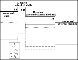
Figure 1: Flow structure near the front part of a relativistic shell moving through an ambient medium (to the right). The initial density and pressure of the shell is $1000$ times larger than that of the ambient medium. The shell propagates with a Lorentz factor $\Gamma=17$, and the initial ratio of pressure and rest-mass energy density is $10^{-4}$. Two shocks form, a reverse shock (RS) propagating into the shell, and a forward shock (FS) propagating into the ambient medium. The shocked shell and the ambient medium are separated by a contact discontinuity (CD). The various lines show (from top to bottom) the rest mass density (thick solid line), the thermal pressure (thick dotted line), the ratio of thermal pressure and rest mass energy (thin solid line), the magnetic pressure (thin dashed line), and the ratio of magnetic energy density and thermal energy density (thin dotted line) using arbitrary units.

A prototypical evolution of the front edge of a shell is shown in Fig. 1. In the particular case displayed here, the external medium is assumed to be at rest, while the shell moves with $\Gamma=17$. Both its density and pressure are $1000$ times larger than in the ambient medium. Inside the shell as well as in the ambient medium the magnetic field strength is such that $\alpha_{\rm B}=10^{-3}$. The thermal pressure is $1.11\times 10^{-3}\rho$ everywhere. Under these conditions two shocks form, a forward and a reverse one, which are separated by a contact discontinuity, and which propagate into the ambient medium and into the shell, respectively. The structure is qualitatively similar to the one found in the pure RHD case (see e.g., Fig. 2 of MAMB04). However, the shocks are not purely hydrodynamic ones, but fast hydromagnetic shocks. Thus, they amplify the magnetic field due to the compression of the plasma: the front shock compresses the magnetic field of the ambient medium (if non-zero), while the reverse shock amplifies the shell’s magnetic field.

The ratio of the magnetic energy density and the thermal energy density $\alpha_{\rm B}$ (thin dotted line in Fig. 1) decreases in the shocked regions. The magnetization parameter $\sigma$ increases in the shocked shell since $B/(\rho\Gamma)$ is uniform across shocks and rarefaction when the magnetic field is perpendicular to the velocity (Romero et al. 2005), i.e., $\sigma\propto B^{2}/\rho\propto\rho$. The particular case shown in Fig. 1 represents the qualitative evolution of a single shell. However, as the quantitative properties of the shocked region depend on the Lorentz factor of the shell, we have performed a parameter study to determine these. The four panels of Fig. 2 show the variation of the density, the pressure, and the magnetization parameter $\alpha_{\rm B}$ in the shocked regions (measured relative to the corresponding quantities in the unshocked regions) with the shell Lorentz factor. Several remarkable points can be inferred from Fig. 2:

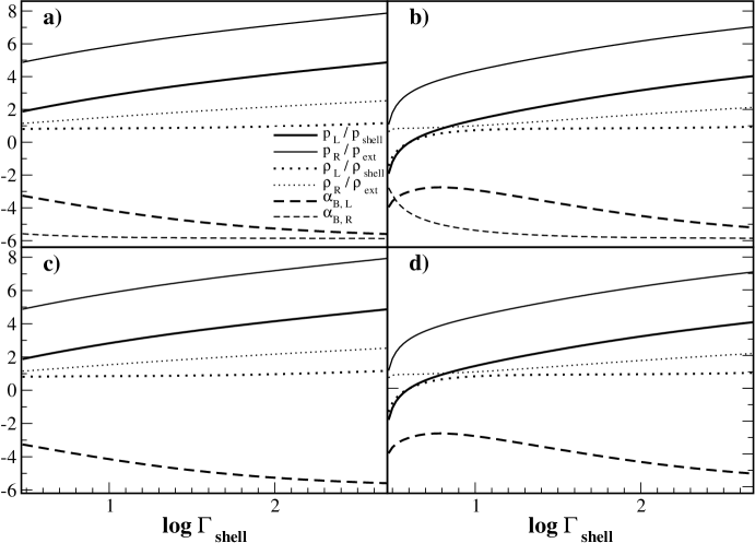
Figure 2: Variation of the logarithms of $\rho_{L}/\rho_{\rm shell}$, $\rho_{R}/\rho_{\rm ext}$, $p_{L}/p_{\rm shell}$, $p_{R}/p_{\rm ext}$, $\alpha_{\rm B,L}$, and $\alpha_{\rm B,R}$ as a function of the shell Lorentz factor, $\Gamma_{\rm shell}$. Subscripts $L$ and $R$ denote the shocked regions to the left and right of the contact discontinuity, respectively. The density and the pressure of the shell are $1000$ times larger than in the ambient medium, and $\alpha_{\rm shell}=10^{-3}$ (as in the case shown in Fig. 1). The parameters of the ambient medium are: (a) $(\Gamma_{\rm ext},\alpha_{\rm B,ext})=(1,10^{-3})$, (b) $(\Gamma_{\rm ext},\alpha_{\rm B,ext})=(3,10^{-3})$, (c) $(\Gamma_{\rm ext},\alpha_{\rm B,ext})=(1,0)$, and (d) $(\Gamma_{\rm ext},\alpha_{\rm B,ext})=(3,0)$, respectively.

1. The ratio of the thermal pressure in the shocked shell region and the initial pressure rises with the Lorentz factor. Even for relatively small Lorentz factors ($\lower 2.15277pt\hbox{$\;\buildrel>\over{\sim}\;$}5$) the thermal pressure is $100$ times larger than the initial one in the case of an ambient medium at rest. The pressure of the ambient medium rises $100$ to $10^{4}$ times above its initial value. In the case of a moving ambient medium and for shell Lorentz factors $\lower 2.15277pt\hbox{$\;\buildrel<\over{\sim}\;$}4$ a rarefaction instead of the reverse shock forms ($\rho_{\rm L}/\rho_{\rm shell}<1$; flow structure $\leftarrow\cal{R}\cal{C}\cal{S}\rightarrow$), while for larger Lorentz factors the situation is as shown in Fig. 1 ($\leftarrow\cal{S}\cal{C}\cal{S}\rightarrow$).

2. A comparison of panels (a) and (c), or (b) and (d) shows that the properties of the shocked shell region only weakly depend on the magnetization of the ambient medium provided the latter is initially sufficiently small ($\alpha_{\rm B,ext}\leq 10^{-3}$) and the shell has $\Gamma_{\rm shell}\lower 2.15277pt\hbox{$\;\buildrel>\over{\sim}\;$}5$, i.e., an initially weakly magnetized ambient medium has no influence on the evolution of the shell.

3. The rest mass density in the shocked part of the shell (L-region in Fig. 1) is independent of the Lorentz factor for $\Gamma\lower 2.15277pt\hbox{$\;\buildrel>\over{\sim}\;$}5$. The comoving magnetic field $B^{\prime}=B/\Gamma$ is independent of the shell Lorentz factor, too, since $B^{\prime}/\rho=constant$ across shocks for magnetic fields perpendicular to the velocity field. Since $\alpha_{\rm B}\propto\rho^{2}/p$, $\rho_{\rm L}\simeq constant$, and $p_{\rm L}$ is monotonically increasing, $\alpha_{\rm B,L}$ decreases monotonically in the L-region.

The latter fact must be taken into account in the internal shock scenario to properly estimate the strength of the magnetic field of the faster shell at the moment when the interaction starts (i.e., when its front edge starts colliding with the back edge of the slower shell), since the magnetic field will be larger, and $\alpha_{\rm B}$ will be smaller than their corresponding initial values.

If a value $\chi_{\rho}>10^{3}$ were used, the leading edges of both shells would develop a Riemann fan with the same qualitative structure. However, relative to the shell flow the two shocks emerging from the leading edges will propagate much more slowly, and accordingly the width of the Riemann fan will be smaller, too. In the limit $\chi_{\rho}\rightarrow\infty$ the width of the fan tends to zero, and the shells behave as rigid bodies propagating through the vacuum (which is the typical assumption made in analytic models of colliding shells).

Zhang & Kobayashi (2005) have considered in detail the dependence of various flow parameters on the relative Lorentz factor between the shell and the ambient medium, and on the magnetization parameter $\sigma$. They also find that for a sufficiently large Lorentz factor, appropriately normalized flow parameters are insensitive to the Lorentz factor, depending only on the magnetization. For example, the dependence of the ratio of magnetic pressure and thermal pressure in the shocked region of the shell (see panel (e) in Fig. 1 of their paper) is consistent with the trend exhibited in Fig. 2

4 Numerical simulations

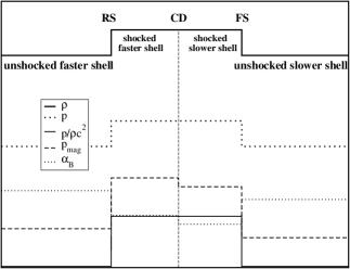
Figure 3: Same as Fig.  1, but for the flow structure near the interface of two interacting shells (assuming no evolution prior to interaction). The initial density, pressure and comoving magnetic field are assumed to be the same in both shells. The Lorentz factor of the faster (left) shell is $7$, and that of the slower (right) shell is $5$.

As in MAMB05, we simulate shell collisions in one spatial dimension only. This approach is justified as all essential features of the collision of aligned shells can be captured in one dimension, since the lateral expansion is negligible during the collision.

The computational grid consists of $10^{4}$ equidistant zones covering a physical domain of length $5\times 10^{15}\,$cm. A grid re-mapping technique (MAMB04) is applied in order to follow the evolution of two shells initially separated by $10^{14}$ cm up to distances of $10^{17}$ cm with sufficiently good resolution.

The energy distribution of the non-thermal electrons is sampled by 64 logarithmically spaced energy bins, and the synchrotron radiation is computed at 40 frequency values logarithmically spanning the frequency range from $10^{15}\,$Hz to $10^{20}\,$Hz. We use the type-E shock acceleration model of MAMB04, with some modifications as explained below.

The RMHD conservation laws are integrated and the synchrotron radiation is computed using MRGENESIS, which is an extension of the RMHD version of the RHD code GENESIS (Leismann et al. 2005). For the adiabatic index of the plasma a value $\gamma_{\rm ad}=4/3$ is assumed. The handling of the non-thermal particles and the computation of the non-thermal emission follows the procedure described in MAMB04, except for the following two modifications:

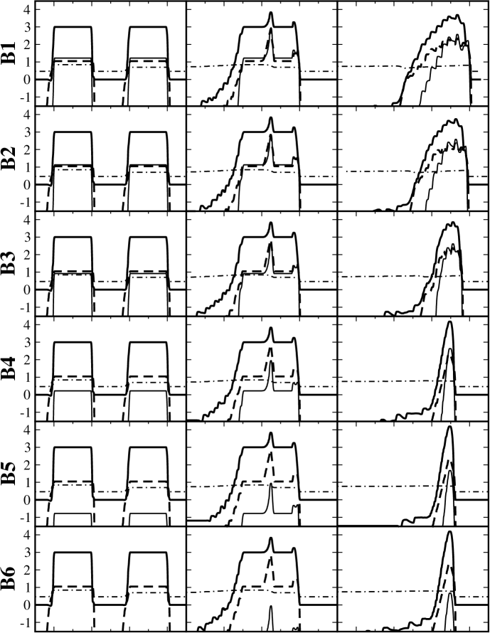
Figure 4: Three snapshots from the evolution of models B1-B6. The thick solid line shows the logarithm of the rest-mass density, the dashed line the thermal pressure, the thin solid line the comoving magnetic field energy density, and the dash-dotted line the Lorentz factor, respectively. The panels in the first column display the situation $1.5\,$ks after the start of the simulations, the second column after $500\,$ks, and the third column after $2000\,$ks (all times are measured in the source frame). The size of the horizontal axis corresponds to a length of $4\times 10^{14}\,$cm.

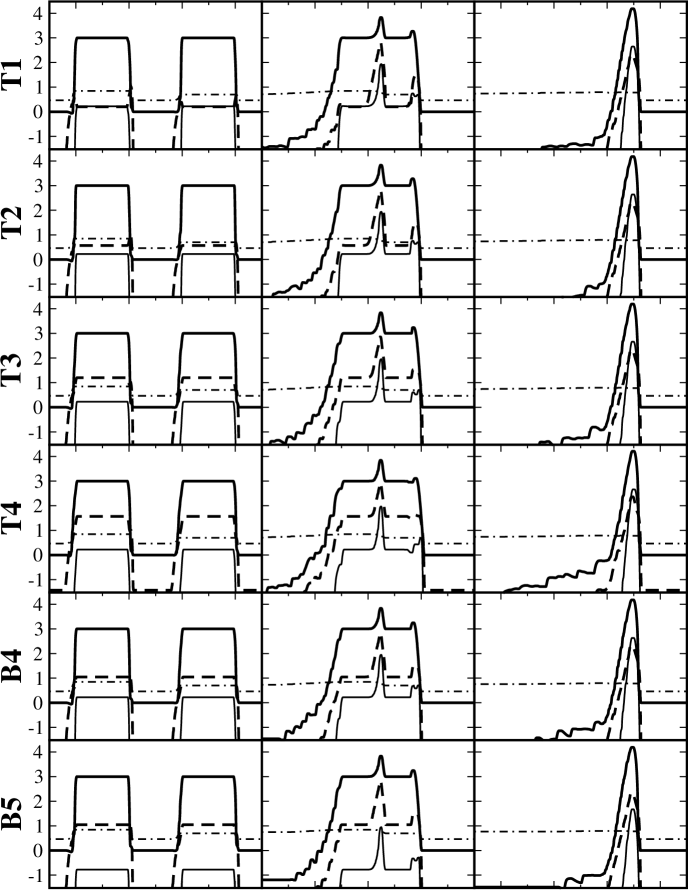
Figure 5: Same as Fig. 4, but for models T1-T4. The snapshots from models B4 and B5 are shown here again to allow for an easier comparison between the models of the T and B series.

1. Synchrotron radiation: for each grid zone the dynamically evolving magnetic field ${\mathbf{B}}$ (measured in the source frame) is transformed into the comoving frame defined by the flow velocity ${\mathbf{v}}$ (or Lorentz factor $\Gamma$) of the zone in order to compute the synchrotron emissivity according to Eq. 14 of MAMB04. However, instead of the magnetic field in the comoving frame $B^{\prime}$ we insert $B^{\prime}\sin\theta^{\prime}$, where $\theta^{\prime}$ is the angle (in the comoving frame) between the line of sight towards the observer and the magnetic field vector. In the present work the flow is assumed to be propagating towards an observer and parallel to the line of sight. Since also the magnetic field is assumed to be initially perpendicular to the direction of the flow, we get $B^{\prime}=B/\Gamma$ and $\theta^{\prime}=\pi/2$.

2. Acceleration of non-thermal particles: we assume that non-thermal particles are accelerated in the shocks that are detected in the magnetized flow with the standard PPM routines implemented in GENESIS (Aloy et al. 1999). However, we replace the jumps in gas pressure by the jumps in total pressure ($p^{*}\equiv p+p_{\rm mag}$) in the shock detection algorithm.

4.1 Magnetohydrodynamic evolution

Figure 3 shows an example of the analytic solution of the interaction of two shells, assuming they have undergone no evolution prior to their collision. This is an approximation of the more realistic situation where the pre-collision evolution changes the conditions at the edges of the shells that are interacting, which is the case of the detailed numerical simulations presented here and in MAMB05. Nonetheless, this approximation captures the qualitative structure of the Riemann fan emerging from interacting over-dense shells and, particularly the fact that the density jump at the contact discontinuity is expected to be small (which can also be seen in the results of our numerical simulations; Figs. 4 and 5, where the evolution prior to collision was taken into account).

Figures 4 and 5 show three snapshots of the magnetohydrodynamic evolution of the $10$ models considered in this work. The left column displays the initial state, the middle column the propagation of the internal shocks through the shells after $500$ ks, and the right column the break out of the shocks from the merged shell after $2000$ ks.

In the middle column the two internal shocks flanking the dominant peak inside the shells can be noticed (corresponding to the region between RS and FS in Fig. 3) as well as the front structure of the slower (right) shell, which arises from the interaction of the shell with the ambient medium (see also Fig. 1). For models T1 - T4 the thermal pressure within the front structure is different, i.e., larger values of $\alpha_{\rm B}^{0}$ (for a fixed magnetic field; see Table 1) yield a greater thermal pressure contrast between the slow shell and the shocked ambient medium ahead of it. Analytically, it is possible to show that the reverse shock propagates more slowly through the merged shell as $\alpha_{\rm B}^{0}$ decreases. This trend is exhibited by the models of the B–series (Fig. 4), where $\alpha_{\rm B}$ decreases from $10^{-1}$ (model B1) to $10^{-4}$ (model B6; see Table 1).

For the models of the T-series the differences in the morphology and the dynamics of the merged shell are not as pronounced as for the B-models, because the initial magnetization of the former models differs only by a fraction $\alpha_{\rm B}^{0}(T1)/\alpha_{\rm B}^{0}(T4)\approx 20$, while $\alpha_{\rm B}^{0}(B1)/\alpha_{\rm B}^{0}(B4)\approx 10^{3}$. However, the slowest shell of model T4, which has the largest thermal pressure, develops a reverse rarefaction instead of a shock as a result of its interaction with the external medium (see middle panel of Fig. 5), although this difference does not have any noticeable influence on the long term evolution of the merged shell. More relevant in the T-series is the near independence of the results on the initial ratio $(p/\rho)^{0}$. Hence, if the initial shells are sufficiently “cold” (i.e., $(p/\rho)^{0}\lower 2.15277pt\hbox{$\;\buildrel<\over{\sim}\;$}10^{-3}$) the exact value of $p$ does not influence the evolution. This implies that it may be impossible to infer the (absolute) value of the initial shell pressure from observations.

The final thickness of the merged shells (after 2000 ks) depends monotonically on $\alpha_{\rm B}^{0}$, because the total pressure $p_{\mathrm{tot}}=p\,\{1+\alpha_{\rm B}/[2(\gamma_{\rm ad}-1)]\}$ increases with $\alpha_{\rm B}^{0}$. Model B1, which has the largest initial magnetization of all models ($\alpha_{\rm B}^{0}=0.1$), gives rise to the thickest merged shell with $\sim 2\times 10^{14}\,$cm, which is of the order of the sum of the initial sizes of the colliding shells. Model B6 produces the thinnest merged shell with $\sim 7\times 10^{13}\,$cm, which is less than the initial size of a single shell. Hence, the final size of the merged shells differs little from the sum of the sizes of the two initial shells. This can be understood from the fact that the final size of the merged shells results from the competition of two factors: the expansion triggered when the colliding shells are heated up by internal shocks, and the compression produced by the collision.

4.2 Energy conversion efficiency

In MAMB05 we monitored the efficiency of the conversion of bulk kinetic energy into internal energy during the collision of the shells. The knowledge of the efficiency is relevant to make predictions about the amount of radiated energy in any model invoking internal shocks as the primary source of the non-thermal emission of an astrophysical plasma. Here we extend our previous study to magnetized shells, i.e., the bulk kinetic energy of the shells can be converted either into thermal energy or into magnetic energy.

We fist define the total instantaneous efficiency of converting bulk kinetic energy into magnetic and thermal energy as

$$\epsilon(T):=1-\displaystyle{\frac{\int\Gamma(z,T)(\Gamma(z,T)-1)\ \rho(z,T)\ {\rm d}z}{\int\Gamma(z,0)(\Gamma(z,0)-1)\ \rho(z,0)\ {\rm d}z}}\,.$$ (4)

Next, using the standard relativistic magnetohydrodynamic expression for the total energy density measured in the laboratory frame $\tau:=\rho{\tilde{h}}\Gamma^{2}-p-p_{\rm mag}-\rho\Gamma$ (where ${\tilde{h}}:=1+\gamma_{\rm ad}p/((\gamma_{\rm ad}-1)\rho)+\sigma$ is the total enthalpy per unit of mass including the magnetic contribution), we can identity the terms corresponding to the kinetic, the thermal and the magnetic energy densities. Taking into account that initially there is not only kinetic energy in the flow but also thermal and magnetic energy, we define the efficiency of converting kinetic energy into thermal energy as

$$\begin{array}[]{rcl}\epsilon_{\rm th}^{\prime}(T)&:=&\biggl{[}\displaystyle\int\ \left(\displaystyle{\frac{\gamma_{\rm ad}}{\gamma_{\rm ad}-1}}\Gamma^{2}(z,T)-1\right)\ p(z,T)\ {\rm d}z\\ &&-\displaystyle\int\ \left(\displaystyle{\frac{\gamma_{\rm ad}}{\gamma_{\rm ad}-1}}\Gamma^{2}(z,0)-1\right)\ p(z,0)\ {\rm d}z\biggr{]}\\ &&\displaystyle/\displaystyle\int\ \Gamma(0,T)(\Gamma(0,T)-1)\ \rho(0,T)\ {\rm d}z\end{array}\,,$$ (5)

and the efficiency of converting kinetic energy into magnetic field energy as

$$\begin{array}[]{rcl}\epsilon_{\rm mag}^{\prime}(T)&:=&\biggl{[}\displaystyle\int\ \left(1-\displaystyle{\frac{1}{2\Gamma^{2}(z,T)}}\right)\displaystyle{\frac{B^{2}(z,T)}{4\pi}}\ {\rm d}z\\ &&-\displaystyle\int\ \left(1-\displaystyle{\frac{1}{2\Gamma^{2}(z,0)}}\right)\displaystyle{\frac{B^{2}(z,0)}{4\pi}}\ {\rm d}z\biggr{]}\\ &&\displaystyle/\int\ \Gamma(0,T)(\Gamma(0,T)-1)\ \rho(0,T)\ {\rm d}z\end{array}\,,$$ (6)

respectively. The quantities $\Gamma$, $p$, $\rho$, and $B$ that appear in the integrals are measured either at time $t=T$ or at time $t=0$, and at position $z$. The integrals in Eqs. 5 and 6 should extend over the whole domain swept up by the shells until the end of the simulation, but we restrict the domain of evaluation to that of the instantaneous computational grid. This restriction is justified since the dominant contribution to the energy (either kinetic, thermal or magnetic) comes from the shells and the shocked ambient medium, which are both always covered by the computational grid, regardless of the grid-remapping (see above). The contributions ignored due to grid-remapping are thus negligible regarding the dynamic evolution of the system, but may effect the efficiencies as they are of the same order of magnitude ($\lower 2.15277pt\hbox{$\;\buildrel<\over{\sim}\;$}1\%$). Therefore, we re-define the efficiencies given in Eqs.5 and 6 by scaling them with $\epsilon(T)$, i.e.,

$$\epsilon_{\rm th}(T)=\displaystyle{\frac{\epsilon_{\rm th}^{\prime}(T)}{\epsilon_{\rm th}^{\prime}(T)+\epsilon_{\rm mag}^{\prime}(T)}}\epsilon(T)\,,$$ (7)

and

$$\epsilon_{\rm mag}(T)=\displaystyle{\frac{\epsilon_{\rm mag}^{\prime}(T)}{\epsilon_{\rm th}^{\prime}(T)+\epsilon_{\rm mag}^{\prime}(T)}}\epsilon(T)\,.$$ (8)

Figs. 6 and 7 show the evolution of $\epsilon_{\rm th}$ (upper panel) and $\epsilon_{\rm mag}$ (lower panel) for models B1 to B6, and models T1 to T4, respectively. From the upper panel of Fig. 6 one infers that the efficiency decreases with $\alpha_{\rm B}$ at late times for all models. The lower panel of Fig. 6 displaying the conversion of kinetic energy into magnetic field energy confirms that models with $\alpha_{\rm B}\leq 0.01$ behave qualitatively differently from models with $\alpha_{\rm B}>0.01$, as the global maximum of the efficiency of the latter models is shifted to earlier times than in models with $\alpha_{\rm B}\leq 0.01$. The upper panel of Fig. 7 shows that the thermal efficiencies $\epsilon_{\rm th}$ of models T1 to T4 are similar to that of model B4, and that the evolution is almost identical for all four models. The efficiency $\epsilon_{\rm mag}$ (lower panel) is generally larger for a lower initial thermal pressure (see Table,1).

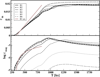
Figure 6: Efficiency of converting bulk kinetic energy into thermal (upper panel) and magnetic field energy (lower panel) for models of the B-series. Times are measured in the source frame. The thick grey line gives an analytic approximation (see Appendix A for details).

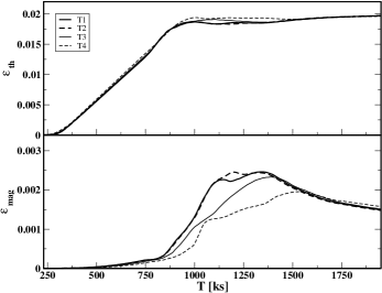
Figure 7: Same as Fig. 6, but for models of the T-series. The graphs for models B4 and B5 are added for comparison.

In Appendix A we give the details of an analytic approximation to compute the efficiencies. The approximation takes into account that the shells are compressible fluids and not solids that collide inelastically, as has been widely assumed in the literature. The thick grey line in Fig. 6 shows our analytic approximations for $\epsilon_{\rm th}$ (upper panel) and $\epsilon_{\rm mag}$ (lower panel), respectively. The parameters for the analytic model are the same as in model B1.

4.3 Light curves

For each model two light curves were computed, one in the energy range $0.1-1$ keV (soft band), and second one in the energy range $2-10$  keV (hard band). The bands are defined to approximately match those used by Brinkmann et al. (2005) when analyzing their observations. As described in detail in MAMB04, light curves are computed by summing the contributions of the emissivity from each grid zone in each time step taking into account the light travel time to the observer.

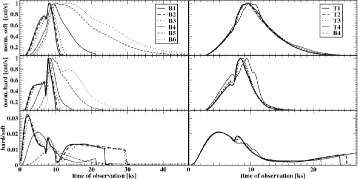
Figure 8: Normalized soft (top) and hard (middle) light curves, and instantaneous hardness ratio (bottom) for models B1 - B6 (left), and T1 - T4 and B2 (right), respectively. Note that all light curves have been normalized individually.

Figure 8 shows the normalized soft (upper panels) and hard (middle panels) light curves of our $10$ models. The difference between the light curves of the B-models (left) and T-models (right) is obvious, as well as their similarity for all T-models and model B4. The instantaneous hardness ratio (HR), defined as the ratio of hard and soft counts at a given observational time (see bottom panels) rapidly rises during the collision phase, and then decreases with the observational time. Hence, at late times ($t\lower 2.15277pt\hbox{$\;\buildrel>\over{\sim}\;$}15\,$ks) the detected radiation becomes softer. Indeed, for models B1 to B3 the light curves and the hardness ratio have a multi-peaked structure, a behavior which has been observed for Mrk 421 (Brinkmann et al. 2005) or PKS2155-304 (Zhang et al. 2006). In these models having a high magnetization ($\alpha_{\rm B}>5\times 10^{-2}$) the relative amount of radiation emitted in both bands changes rapidly with time. Models with $\alpha_{\rm B}>10^{-2}$ show a persistent, moderately high hardness ratio ($>0.01$) at late epochs ($t>15\,$ks), which correlates with the fact that the RMHD evolution of the merged shell produced by initial shells with $\alpha_{\rm B}<10^{-2}$ is characterized by a long-persisting structure radiating dominantly in the soft band (see Sect. 5.3). T-models, all of them with low initial magnetic field (equal to that of model B4) do not exhibit a variable behavior but the same smooth trends as models B5 and B6.

5 Discussion

In the following sections we will summarize the main results of our numerical investigation.

5.1 Magnetohydrodynamic evolution

MAMB05 found that the relativistic hydrodynamic (RHD) evolution of shell interactions can be divided into three phases: pre-collision, collision, and post-collision (rarefaction) phase. The evolution of magnetized shells also exhibits these three phases, but with some differences.

5.1.1 Pre-collision phase

Since the magnetic field inside the shell is perpendicular to the direction of motion, the initially sharp forward edge of the shell develops into a Riemann fan consisting of three simple waves, namely two magnetosonic shocks separated by a contact discontinuity (Fig. 1). The reverse shock compresses the shell as it propagates towards the shell’s rear edge. The compression factor ($\rho_{\rm L}/\rho_{\rm shell}$) is almost independent of the Lorentz factor leveling off to a value $\sim 10$ when $\Gamma_{\rm shell}\lower 2.15277pt\hbox{$\;\buildrel>\over{\sim}\;$}5$ (Fig. 2). As the ram pressure exerted by the ambient medium is proportional to $\rho\Gamma^{2}$, the pressure increase in the shocked regions rises with the Lorentz factor faster than the density yielding a strong heating of the shell’s edge. Since the ratio of the magnetic field and the rest mass density remains constant on both sides of the contact discontinuity, the magnetization parameter $\alpha_{\rm B,L}$ is reduced in the shocked ambient medium by up to two orders of magnitude for high Lorentz factors ($\Gamma_{\rm shell}\lower 2.15277pt\hbox{$\;\buildrel>\over{\sim}\;$}100$; see panels (a) and (c) in Fig. 2). This decrease of $\alpha_{\rm B,L}$ is important in those cases where the shells take a long time to collide, since the reverse shock (originating from the interaction with the ambient medium) can traverse a substantial part of the faster shell before collision.

While shell heating also occurs for non-magnetized shells, the pre-collision evolution of magnetized shells is further characterized by an increase of the magnetization parameter $\sigma_{\rm L}$ in the shocked part of the shell (see Sec. 3), because $\sigma_{\rm L}$ is proportional to the rest-mass density when the field is oriented perpendicular to the direction of motion. On the other hand, the ratio of magnetic energy density and thermal energy density $\alpha_{\rm B,L}$ decreases as the jump in the thermal pressure in the shocked region is larger than the jump in density, and thus also larger than the jump in the magnetic field. Consequently, at the onset of the collision phase the magnetic field of the faster shell is larger but dynamically less important than the shell’s initial field. The properties of the shocked shell (magnetization parameters, density contrast with respect to the shell, pressure jump, etc.) depend only weakly on its Lorentz factor when the latter becomes large. This fact is of special relevance in the case of GRB afterglows, which may arise from the evolution of a single shell moving initially with a Lorentz factor $\Gamma\sim 100$. The properties of the shocked shell are then largely determined by the magnetization parameter $\sigma$ and its density contrast with respect to the ambient medium.

5.1.2 Collision phase

Figs. 4 and 5 (middle column) demonstrate that the ratio of the magnetic field energy density (thin solid line) and the pressure (thick dashed line) has decreased at the collision phase relative to its initial value (first column), consistent with what is seen in Fig. 3 (the thin dotted line, denoting $\alpha_{\rm B}$, decreases in shocked regions). The spatial distribution of the thermal pressure in the region limited by the internal shocks (created during the collision) is very similar for all models. However, the shock structure of the slower shell resulting from its interaction with the ambient medium is characterized by a larger jump in the thermal pressure jump in models with larger initial magnetic fields.

For the conditions considered in our models, which correspond to the typical values expected in blazars, maximum efficiencies of conversion of kinetic into thermal energy of $\sim 2\%$ are found. Much smaller values are computed for the conversion of kinetic into magnetic energy ($\sim 0.2\%$). According to our analytic model (see Appendix A), the maximum efficiencies of conversion of kinetic into thermal energy may rise up to $\sim 10\%$ for the typical conditions expected for internal collisions in GRBs, while the efficiency of conversion of kinetic into magnetic energy decreases to $\epsilon_{\rm mag}\lower 2.15277pt\hbox{$\;\buildrel<\over{\sim}\;$}8\times 10^{-5}$.

5.1.3 Post-collision phase

Once the internal shocks break out of the merged shell, they rapidly stretch it, lowering its mean density and, in general, producing rarefaction waves in the rear part of the merged shell (similar to what MAMB05 found in the pure RHD case). At source frame times later than $\approx 1500\,$ks corresponding to a few sound crossing times of the merged shells the lateral expansion of the shocked regions can be significant, i.e., the synchrotron luminosity is overestimated, and the size and thermodynamic properties of the merged shells have to be considered with care. Indeed, overestimating the pressure and the density in the region bounded by internal shocks could be the reason for some features observed at very late times in our synthetic light curves and in the hardness ratio (e.g., the secular increase of the hardness ratio in the T-models).

5.2 Evolution of the magnetic field

The evolution of the magnetization parameter $\alpha_{\rm B}$ at the point of maximum magnetic field at any given instant of time in the source frame shows two epochs separated by a sharp discontinuity at about $300\,$ks (Fig. 9). The instantaneous location of the maximum magnetic field is indicative of the region which instantaneously (in the source frame) contributes most to the radiated energy. Hence, it is a representative point of the binary shell evolution.

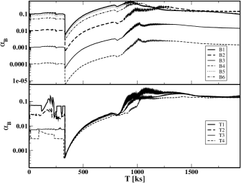
Figure 9: Ratio of the comoving magnetic energy density and the thermal energy density $\alpha_{\rm B}$ as a function of time in the source frame for the grid point with the maximum magnetic field. The upper panel shows the B-models which all have the same initial pressure, and the lower panel displays the T-models which all have the same initial magnetic field.

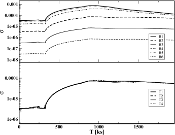
Figure 10: Same as Fig. 9 but showing the time evolution of the ratio of the comoving magnetic energy density and the kinetic energy density.

Left of the discontinuity the maximum magnetic field is produced by the reverse shock (caused by the interaction with the ambient medium) of the faster shell prior to the collision as it compresses the fluid in the shell. The part right of the discontinuity corresponds to a point inside the reverse internal shock formed during the collision phase (see Sec. 5.1). The sharp discontinuity in $\alpha_{\rm B}$ occurs when the global maximum of the magnetic field shifts from the external shock region of the faster shell to the internal shock region of the merged shell.

All curves shown in the upper panel of Fig. 9 are qualitatively very similar, especially regarding the relative magnitude of the sharp drop in $\alpha_{\rm B}$ at $\leavevmode\nobreak\ 300\,$ks, which is almost identical for all the B-models. This implies that the system does not completely “forget” its initial conditions. Although inside the region shocked by internal shocks $\alpha_{\rm B}$ is about one order of magnitude smaller than the initial magnetization $\alpha_{\rm B}^{0}$ in the shell, the ordering of the models according to $\alpha_{\rm B}^{0}$ is preserved, at least until $\alpha_{\rm B}$ reaches its maximum value at $t\sim 900\,$ks.

The second magnetization parameter $\sigma^{0}$ is non degenerate in the B-models (Fig. 10, upper panel), since during the collision kinetic energy is dissipated, increasing the magnetic field in the shocked region, while the initially small thermal energy component has very little influence.

A qualitatively different behavior is observed for the models of the T-series (Fig. 9, lower panel). These have a different initial magnetization parameter $\alpha_{\rm B}^{0}$, but the absolute value of the magnetic field is initially the same in these models. Thus, $\alpha_{\rm B}$ evolves very similarly in these models after the discontinuity in $\alpha_{\rm B}$ is encountered. The evolution of $\sigma$ is degenerate (see lower panel of Fig. 10), since all models have the same initial value $\sigma^{0}$ and undergo an almost indistinguishable evolution.

We therefore conclude that, in order to describe the essentials of the magnetohydrodynamic properties of binary collisions of cold shells, one can safely exclude the initial thermal pressure (or, equivalently, the internal energy) as a relevant parameter, and may use some canonical value instead, which is sufficiently small compared to the kinetic energy.

5.3 Radiation

The light curves of all models having the same initial magnetic field look similar (Fig. 8; right panels), which is consistent with the picture described in Sect. 5.2, as during the collision phase the initial value of $\sigma$ is the relevant parameter to account for the magnetic field evolution. For large values of $\sigma$ the light curves are shorter and multi-peaked, while for decreasing $\sigma^{0}$ they become single-peaked and have a longer decreasing tail which is progressively softer (Fig. 8; left panels). The border separating cases with a multi-peaked or mono-peaked light curve is given by the combination of the value of $\sigma$ and a critical value of $\alpha_{\rm B}^{0}$ of the order of $10^{-2}$ (see Sect. 4.3).

Comparing the light curves of the current work with those given in Fig. 4 of MAMB05, we find that also in the magnetized case hard light curves are shorter in duration than soft ones, and that only low magnetization ($\alpha_{\rm B}^{0}\leq 10^{-2}$) models have a shape similar to those of MAMB05, which is not surprising since in the limit of $\alpha_{\rm B}^{0}\rightarrow 0$ the pure hydrodynamic limit must be recovered. As can be seen when comparing the lower panels of Fig. 8 with the lower panel of Fig. 4 of MAMB05, the initial rise of the hard light curves is not smooth, but exhibits a small ’kink’ both for non-magnetized and magnetized models. This similarity indicates that the assumptions made in MAMB05 are valid for small $\alpha_{\rm B}^{0}$, but need not necessarily hold for high initial $\alpha_{\rm B}^{0}$, too.

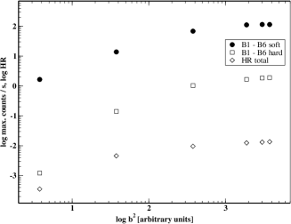
Figure 11: Maxima of soft (filled circles) and hard (squares) light curves for models B1 to B6 as a function of the square of the initial comoving magnetic field. The total hardness ratio (HR) is defined as the ratio of the time-integrated number of counts in the hard and in the soft bands, respectively. It is displayed with the diamond symbols.

The maxima of the soft and of the hard light curves, as well as the total hardness ratio (ratio of the time-integrated number of counts in the hard and in the soft bands) depend on the initial magnetic field for the B-models (Fig. 11). Our models show that the maxima of the light curves have a logarithmic-like dependence on the initial magnetic field energy density. In order to explain the weaker dependence of the light curve maxima and hardness ratio on the magnetic field for increasing magnetization, we approximate the typical high-energy synchrotron spectrum (Fig. 12) as a broad peak with a power-law decay towards higher photon energies. The position of the peak shifts to higher energies for larger values of the magnetic field. . For models with lower magnetic fields the part of the spectrum in the hard observational band is the power-law tail resulting in a strong dependence of the light curve on the value of the magnetic field during the evolution. For the high magnetic field models, the maximum of the spectrum partly extends into the hard band, i.e., increasing the magnetic field does not change the observed energy in the hard band as dramatically as in the previous case. This can explain the saturation of the dependence of the hardness ratio on the magnetic field.

Here we stress once more that the light curve at any given time is the result of the sum of the emission from different points radiating at different times in the source frame. This explains why, e.g., the spectrum of model B1 (Fig. 12) has a more complicated shape than that of model B6. Nevertheless, our basic conclusion about the dependency on the magnetic field should hold in both cases.

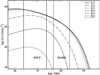
Figure 12: Spectra at the soft light curve maximum for models of the B-series. In order to provide an absolute luminosity scale we assume a shell radius $R_{\mathrm{s}}=10^{17}\,$cm. The edges of the soft and hard observation bands are indicated by two pairs of vertical lines.

A similar study as for the B-models has been done for the light curve maxima of models T1 to T4 as a function of the initial thermal pressure. A very weak dependence of the radiation on the initial (small) pressure was found, which is consistent with the discussion of Sec. 5.2 about the importance of the initial value of $\sigma$ and the unimportance of $\alpha_{\rm B}^{0}$ for the collision dynamics and the emitted radiation.

5.4 On the energy subtraction mechanism

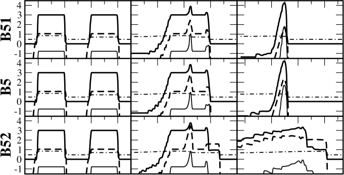
Figure 13: Same as Fig. 4 but for model B5 (middle column) and two additional models: model B51 with $\alpha_{\mathrm{e}}=0.05$ (left column), and model B52 with $\alpha_{\mathrm{e}}=0.001$ (right column).

The mechanism used by us to extract energy from the thermal plasma and to transfer it to the non-thermal population of radiating electrons is based on the type-E macroscopic recipe proposed by MAMB04. In the type-E model one subtracts from the thermal plasma a fraction $\alpha_{\mathrm{e}}$ of the internal energy dissipated in shocks. This fraction $\alpha_{\mathrm{e}}$ is a parameter of our models which is poorly constrained by the current knowledge of the physics of particle acceleration at shock fronts, a typical value being $\alpha_{\mathrm{e}}\simeq 10^{-2}$. In this subsection we critically discuss the impact of different choices of $\alpha_{\mathrm{e}}$ on the result. To this end we computed two additional models having the same model parameters as model B5, but assuming different values for $\alpha_{\mathrm{e}}$: In model B51 we set $\alpha_{\mathrm{e}}=5\times 10^{-2}$, and in model B52 we choose $\alpha_{\mathrm{e}}=10^{-3}$ (see Fig. 13).

Regarding the physical parameters of shocked regions (i.e., those regions affected by the energy subtraction mechanism) a comparison of the evolution of models B5, B51 and B52 provides the following insights:

1. Increasing the value of $\alpha_{\mathrm{e}}$ yields smaller values of the thermal pressure, i.e., the shocked regions become cooler.

2. The magnetic energy density grows as $\alpha_{\mathrm{e}}$ is increased in the region swept up by internal shocks. This growth is consistent with the fact that a more efficient cooling needs higher magnetic field strengths (because that reduces the cooling time).

3. The size of the region containing the shocked ambient medium ahead of the slower shell (R-region in Fig. 1) increases as $\alpha_{\mathrm{e}}$ decreases, because the amount of cooling is reduced (point 1 above), i.e., the forward shock is not as severely weakened as in models with larger $\alpha_{\mathrm{e}}$. Indeed for $\alpha_{\mathrm{e}}>0.01$ the forward shock is almost suppressed, and thus almost no R-region forms. The increase in size of the R-region leads to a decrease of the density, and consequently of the magnetic field energy density in that region (Fig. 13 panels in middle row). Note that this trend is opposite to the increase of the magnetic field energy density observed in the internal shock region.

4. The state reached by models with different $\alpha_{\mathrm{e}}$ at late epochs is quantitatively very different (Fig. 13 panels in bottom row). The energy subtracted from the merged shell (which is swept up completely by shocks) is higher for increasing values of $\alpha_{\mathrm{e}}$. Hence, the merged shells of models B5 and B51 are much cooler (about one order of magnitude) than that of model B52, i.e., the most evident effect of the shell cooling is the much smaller expansion of the merged shell at late times.

5. The larger the value of $\alpha_{\mathrm{e}}$, the larger is the magnetization parameter $\alpha_{\rm B}$. In the collision phase, $500$ ks after the start of simulation (Fig. 13 panels in middle row), the value of $\alpha_{\rm B}$ at the point having the maximum density (in the internal shock region) is more than one order of magnitude higher for model B51 ($\alpha_{\rm B}=3.4\times 10^{-3}$) than for model B52 ($\alpha_{\rm B}=1.5\times 10^{-4}$). The increase of $\alpha_{\rm B}$ results from the combined effect of the decrease of the thermal pressure (point 1 above) and the increase of the magnetic field strength (point 2 above). This result is consistent with the physical expectation that larger magnetic fields (which, in our case, also imply larger values of $\alpha_{\rm B}$) will cool down the shocked regions faster, i.e., for the same elapsed time, more energy will be radiated away for larger magnetic fields than for smaller ones.

6. The value of $\sigma$ at the point of maximum density is rather insensitive to the choice of $\alpha_{\mathrm{e}}$ (for models B51 and B52 the value of $\sigma$ at $500$ ks is $2.7\times 10^{-6}$ and $2.2\times 10^{-6}$, respectively). This strengthens our argument that $\sigma$ is the appropriate parameter to trace the RMHD evolution of colliding shells, as the ordering of the models according to $\sigma$ remains unchanged even if one varies the value of $\alpha_{\mathrm{e}}$.

5.5 Comparison with blazar properties

5.5.1 Emission properties

For models B1 - B6 the radiative luminosity of a single flare lies in the range $10^{42}-10^{44}$ erg s^-1 assuming a shell radius of $10^{17}\,$cm (Fig. 12). This luminosity roughly agrees with the lower limit observed for the moderately luminous blazars whose synchrotron peak lies in the X-ray band (see e.g., Fossati et al. 1998). As the absolute value of the luminosity depends non-linearly on the parameter $\alpha_{\mathrm{e}}$ (see § 5.4), the efficiency of the conversion of kinetic energy into radiation is somewhat unconstrained. For a homogeneous cylindrical shell with a rest mass density $\rho$, Lorentz factor $\Gamma$, and velocity $v$ the kinetic luminosity can be defined as

$$L_{\rm kin}:=\pi R_{\mathrm{s}}^{2}(\tilde{h}\Gamma-1)\rho\Gamma v\,.$$

For our initial models the kinetic luminosity is $\simeq 2\times 10^{47}$ erg s^-1, implying a conversion efficiency of the order of $0.01\%-0.1\%$ for $\alpha_{\mathrm{e}}=10^{-2}$. We emphasize that although both the kinetic and the radiative luminosities are unconstrained by our one-dimensional simulations up to a factor $\pi R_{\mathrm{s}}^{2}$, their ratio and hence the efficiency of conversion of kinetic into radiative luminosities is independent of this factor.

Our models are set up to have a uniform magnetization $\sigma^{0}$ both in the shells and in the ambient medium. Consequently, once the density of the ambient medium is fixed, the magnetic field strength in the shocked region roughly corresponds to the values inferred from observations of blazars, i.e., $\simeq 0.01-1$ G (e.g., Ghisellini et al. 1998). Increasing the ratio of shell to ambient medium density $\chi_{\rho}$, will increase the kinetic luminosity of the shells proportionally. Assuming a uniform initial magnetization, an increase of $\chi_{\rho}$ will, however, drive the value of the magnetic field in the shocked regions above the aforementioned values. Thus, in order to set up future simulations that mimic more powerful blazars with realistic magnetic field strengths, we will have to consider denser shells whose magnetization parameter $\sigma^{0}$ is smaller than that of the ambient fluid.

The number density of radiating non-thermal electrons is $\lower 2.15277pt\hbox{$\;\buildrel>\over{\sim}\;$}10^{4}-10^{5}\,$cm^-3, which is one or two orders of magnitude higher than the usually inferred values $\lower 2.15277pt\hbox{$\;\buildrel>\over{\sim}\;$}10^{3}-10^{4}\,$cm^-3 (e.g. Ghisellini et al. 1998). However, these values are obtained under the assumption that the emitting region is a sphere, whereas in our case the emitting region is a cylinder whose height $L\sim 10^{14}\,$cm is much smaller than its radius $R_{\mathrm{s}}\sim 10^{17}\,$cm. Hence, for the same number of emitting electrons, the number density of radiating particles in this smaller volume is expected to be larger.

5.5.2 Light curves

Following Brinkmann et al.  (2005), we calculate the cross-correlation function (CCF) of the light curves of models B1 to B6. If the observed counts are binned into $N$ equidistant time intervals $\Delta t$, the CCF is defined as follows,

$$CCF(k\Delta t):=\displaystyle{\frac{\sum_{i}(x_{\rm soft}(i\Delta t)-\bar{x}_{\rm soft})(x_{\rm hard}((i+k)\Delta t)-\bar{x}_{\rm hard})}{n(k\Delta t)\sqrt{\sigma_{\rm soft}^{2}\sigma_{\rm hard}^{2}}}}\,,$$ (9)

where $k=0,1,...,(N-1)$, and $\bar{x}_{\rm soft}$, and $\bar{x}_{\rm hard}$ are the number of counts averaged over the N-intervals for photons detected in the soft and in the hard band, respectively. $\sigma_{\rm soft}$ and $\sigma_{\rm hard}$ are the standard deviations of the samples with respect to the corresponding average number of counts in the soft and hard bands, respectively. $n(k)$ is the number of pairs $(i,i+k)$ where $x_{\rm soft}(i\Delta t)$ and $x_{\rm hard}((i+k)\Delta t)$ are both nonzero for a given $k$. The time interval $k\Delta t$ is called the time lag. Significant correlation at e.g., negative lags implies that soft band variations are observed later than hard band variations.

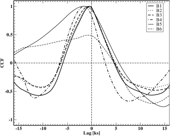
Figure 14: Normalized cross-correlation function (see Eq. 9) for models B1 to B6. Bins of $16.6\,$s were used when computing the cross-correlation functions.

Contrary to the observations shown by Brinkmann et al. (2005; Fig. 3), the maxima of the CCFs are not located at zero time lag, but at negative time lags (Fig. 14), i.e., our simulations only predict the existence of soft lags. However, the overall shapes of the CCF curves are well covered by our models, including both symmetric and asymmetric ones.

For small initial magnetic fields, the CCFs become more asymmetric. Ravasio et al.  (2004) pointed out that the asymmetry can be reproduced by modeling light curves as initially rising linearly, and subsequently decreasing with different time scales at different frequencies. This behavior can be understood from our models as well. For lower magnetic fields the light curve is visible for a shorter time in the hard band than in the soft band (Fig. 12), thus giving rise to different time scales. We point out that these time scales are not only related to the cooling of the relativistic electrons, but to the radial expansion of the emission region as well, whereby the magnetic field inside this region is decreased. The fact that we only see soft lags is probably a consequence of the particular acceleration mechanism model we have chosen (fixed lower and upper limits of the non-thermal electron energy distribution; type-E model of MAMB04). The influence of the acceleration mechanism will be the subject of future work.

5.6 Summary

A detailed study of the interaction of magnetized shells in relativistic outflows has been performed. An idealized interaction of a shell with an ambient medium was studied using an exact Riemann solver (Romero et al. 2005), while the full interaction of two colliding shells was simulated in one spatial dimension using a RMHD code (Leismann et al. 2005) coupled to the synchrotron emission scheme of MAMB04. The models are parametrized to address blazar jets under the hypothesis that blazar light curves result from internal shocks within relativistic jets. However, some results can be extrapolated to the dynamics of internal shocks in GRBs, when taking into account that in the latter case the Lorentz factors are one order of magnitude or more larger than in blazar jets, and that therefore much smaller relative velocities are encountered between the colliding shells.

Appendix A Analytic modeling of energy conversion efficiencies

In this section we idealize the interaction of two colliding shells by neglecting the pre-collision phase, and assuming that the dynamics of the collision can be approximated by solving a Riemann problem at the interface of the two shells. Fig. 15 shows an example of the flow structure in this case. From left to right we identify the following four distinct regions , each with its rest-mass density $\rho$, thermal pressure $p$, magnetic field $B$ (assumed perpendicular to the direction of propagation), and the fluid Lorentz factor $\Gamma$:

1. unshocked faster shell (between $x_{\mathrm{L}}(T)$ and $x_{\mathrm{RS}}(T)$): $\rho_{\mathrm{L}}$, $p_{\mathrm{L}}$, $B_{\mathrm{L}}$, $\Gamma_{\mathrm{L}}$

2. shocked faster shell (between $x_{\mathrm{L}}(RS)$ and $x_{\mathrm{CD}}(T)$): $\rho_{\mathrm{LS}}$, $p_{\mathrm{LS}}$, $B_{\mathrm{LS}}$, $\Gamma_{\mathrm{CD}}$

3. shocked slower shell (between $x_{\mathrm{CD}}(T)$ and $x_{\mathrm{FS}}(T)$): $\rho_{\mathrm{RS}}$, $p_{\mathrm{RS}}$, $B_{\mathrm{RS}}$, $\Gamma_{\mathrm{CD}}$

4. unshocked slower shell (between $x_{\mathrm{FS}}(T)$ and $x_{\mathrm{R}}(T)$): $\rho_{\mathrm{R}}$, $p_{\mathrm{R}}$, $B_{\mathrm{R}}$, $\Gamma_{\mathrm{R}}$

The five (time-dependent) boundaries of the four regions are from left to right:

1. left edge of the faster shell at $x_{\mathrm{L}}(T)=T\sqrt{1-\Gamma_{\mathrm{L}}^{-2}}$

2. reverse shock at $x_{\mathrm{RS}}(T)=\Delta x_{\mathrm{L}}+T\sqrt{1-\Gamma_{\mathrm{RS}}^{-2}}$

3. contact discontinuity at $x_{\mathrm{CD}}(T)=\Delta x_{\mathrm{L}}+T\sqrt{1-\Gamma_{\mathrm{CD}}^{-2}}$

4. forward shock at $x_{\mathrm{FS}}(T)=\Delta x_{\mathrm{L}}+T\sqrt{1-\Gamma_{\mathrm{FS}}^{-2}}$

5. right edge of the slower shell at $x_{\mathrm{R}}(T)=\Delta x_{\mathrm{L}}+\Delta x_{\mathrm{R}}+T\sqrt{1-\Gamma_{R}^{-2}}$,

where $\Delta x_{\mathrm{L}}$ and $\Delta x_{\mathrm{R}}$ are the initial thickness of the faster and of the slower shell, respectively. The reverse shock, the contact discontinuity and the forward shock originate at the interface between the two shells. The origin of the coordinate system coincides with the left edge of the faster shell at $T=0$.

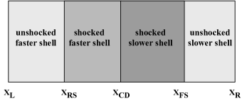
Figure 15: A schematic representation of the idealized interaction of two colliding shells consisting of four distinct regions. The shells are assumed to move towards the right.

Knowing the initial values of $\rho$, $p$, $B$, and $\Gamma$ in the shells, we use the exact Riemann solver (Romero et al. 2005) to compute values in the intermediate states. We then define the total kinetic, thermal and magnetic energy at a time $T$ as follows:

$$\begin{array}[]{rcl}E_{\mathrm{K}}(T)&:=&\Gamma_{\mathrm{L}}(\Gamma_{\mathrm{L}}-1)\ \rho_{\mathrm{L}}\ (x_{\mathrm{RS}}(T)-x_{\mathrm{L}}(T))\\ &&+\Gamma_{\mathrm{CD}}(\Gamma_{\mathrm{CD}}-1)\ \rho_{\mathrm{LS}}\ (x_{\mathrm{CD}}(T)-x_{\mathrm{RS}}(T))\\ &&+\Gamma_{\mathrm{CD}}(\Gamma_{\mathrm{CD}}-1)\ \rho_{\mathrm{RS}}\ (x_{\mathrm{FS}}(T)-x_{\mathrm{CD}}(T))\\ &&+\Gamma_{R}(\Gamma_{R}-1)\ \rho_{\mathrm{R}}\ (x_{\mathrm{R}}(T)-x_{\mathrm{FS}}(T))\end{array}\,,$$ (10)

$$\begin{array}[]{rcl}E_{\mathrm{th}}(T)&:=&\left(\displaystyle{\frac{\gamma_{\rm ad}}{\gamma_{\rm ad}-1}}\Gamma_{\mathrm{L}}^{2}-1\right)\ p_{\mathrm{L}}\ (x_{\mathrm{RS}}(T)-x_{\mathrm{L}}(T))\\ &&+\left(\displaystyle{\frac{\gamma_{\rm ad}}{\gamma_{\rm ad}-1}}\Gamma_{\mathrm{CD}}^{2}-1\right)p_{\mathrm{LS}}\ (x_{\mathrm{CD}}(T)-x_{\mathrm{RS}}(T))\\ &&+\left(\displaystyle{\frac{\gamma_{\rm ad}}{\gamma_{\rm ad}-1}}\Gamma_{\mathrm{CD}}^{2}-1\right)p_{\mathrm{RS}}\ (x_{\mathrm{FS}}(T)-x_{\mathrm{CD}}(T))\\ &&+\left(\displaystyle{\frac{\gamma_{\rm ad}}{\gamma_{\rm ad}-1}}\Gamma_{\mathrm{R}}^{2}-1\right)p_{\mathrm{R}}\ (x_{\mathrm{R}}(T)-x_{\mathrm{FS}}(T))\end{array}\,,$$ (11)

and

$$\begin{array}[]{rcl}E_{\mathrm{mag}}(T)&:=&\left(\Gamma_{\mathrm{L}}^{2}-\displaystyle{\frac{1}{2}}\right)\ \displaystyle{\frac{B_{\mathrm{L}}^{2}}{4\pi}}\ (x_{\mathrm{RS}}(T)-x_{\mathrm{L}}(T))\\ &&+\left(\Gamma_{\mathrm{CD}}^{2}-\displaystyle{\frac{1}{2}}\right)\ \displaystyle{\frac{B_{\mathrm{LS}}^{2}}{4\pi}}\ (x_{\mathrm{CD}}(T)-x_{\mathrm{RS}}(T))\\ &&+\left(\Gamma_{\mathrm{CD}}^{2}-\displaystyle{\frac{1}{2}}\right)\ \displaystyle{\frac{B_{\mathrm{RS}}^{2}}{4\pi}}\ (x_{\mathrm{FS}}(T)-x_{\mathrm{CD}}(T))\\ &&+\left(\Gamma_{\mathrm{R}}^{2}-\displaystyle{\frac{1}{2}}\right)\ \displaystyle{\frac{B_{\mathrm{R}}^{2}}{4\pi}}\ (x_{\mathrm{R}}(T)-x_{\mathrm{FS}}(T))\\ \end{array}\,.$$ (12)

As in Eq. 4, we define the total efficiency for conversion of kinetic into thermal and magnetic energy

$$\epsilon^{\mathrm{an}}(T):=1-\displaystyle{\frac{E_{\mathrm{K}}(T)}{E_{\mathrm{K}}(0)}}\,,$$ (13)

the efficiency of conversion of kinetic into thermal energy

$$\epsilon_{\rm th}^{\mathrm{an}}(T):=\displaystyle{\frac{E_{\mathrm{th}}(T)-E_{\mathrm{th}}(0)}{E_{\mathrm{K}}(0)}}\,,$$ (14)

and the efficiency of conversion of kinetic into magnetic energy

$$\epsilon_{\rm mag}^{\mathrm{an}}(T):=\displaystyle{\frac{E_{\mathrm{mag}}(T)-E_{\mathrm{mag}}(0)}{E_{\mathrm{K}}(0)}}\,.$$ (15)

The gray thick line in Fig. 6 shows $\epsilon_{\rm th}^{\mathrm{an}}$ (upper panel) and $\epsilon_{\rm mag}^{\mathrm{an}}$ (lower panel) for the initial shell set-up of model B1. We assume that the shells collide after a time of $335\,$ks, determined by their initial separation ($10^{14}\,$cm) and Lorentz factors ($7$ and $5$, respectively). We compute the efficiencies until the forward shock reaches the edge of the slower shell, as the analytic approach is no longer valid later on. There is a good agreement between the final value of $\epsilon_{\rm th}^{\mathrm{an}}$ ($0.0191$) and the maximum value of $\epsilon_{\rm th}$ for model B1 ($0.0195$). The slope of the initial efficiency increase is rather well captured, too. The instantaneous discrepancies between the numeric and analytic estimates mostly arise from the pre-collision evolution of the shells.

We have also applied the above method to the conditions expected to be found in GRBs. Defining the relative Lorentz factor of the shells as $\Delta g\equiv(\Gamma_{\mathrm{L}}-\Gamma_{\mathrm{R}})/\Gamma_{\mathrm{R}}$, we show $\epsilon_{\rm th}^{\mathrm{an}}$ and $\epsilon_{\rm mag}^{\mathrm{an}}$ in Fig. 16 assuming a low magnetization parameter $\sigma=3\times 10^{-5}$ and initially cold shells with $p/\rho=10^{-2}$. Different curves correspond to different values of $(\Gamma_{\mathrm{R}},\Delta g)$. Our results show that, for the typical conditions considered for internal shocks in GRBs (e.g., Daigne & Mochkovitch 1998), maximum efficiencies between $6\%$ and $10\%$ can be obtained.

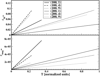
Figure 16: Efficiency of converting bulk kinetic energy into thermal (upper panel) and magnetic field energy (lower panel) as a function of time. Shown are six models with different values of $(\Gamma_{\mathrm{R}},\Delta g)$ and with $\sigma=3\times 10^{-5}$, where $\Delta g\equiv(\Gamma_{\mathrm{L}}-\Gamma_{\mathrm{R}})/\Gamma_{\mathrm{R}}$ is the relative Lorentz factor, and where $\Gamma_{\mathrm{L}}$ and $\Gamma_{\mathrm{R}}$ are the Lorentz factors of the faster and the slower shell, respectively.

Figure 17 shows the maximum efficiencies (corresponding to the final states in Fig. 16) for a fixed Lorentz factor $\Gamma_{\mathrm{R}}$ as a function of the relative Lorentz factor $\Delta g$ keeping all other parameters the same as in Fig. 16. The efficiency depends strongly on $\Delta g$, and is independent of $\Gamma_{\mathrm{R}}$ for large values of $\Delta g$.

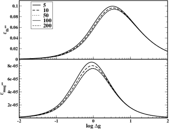
Figure 17: Efficiency of converting bulk kinetic energy into thermal (upper panel) and magnetic field energy (lower panel) as a function of the relative Lorentz factor $\Delta g$, where $\Delta g\equiv(\Gamma_{\mathrm{L}}-\Gamma_{\mathrm{R}})/\Gamma_{\mathrm{R}}$, and where $\Gamma_{\mathrm{L}}$ and $\Gamma_{\mathrm{R}}$ are the Lorentz factors of the faster and the slower shell, respectively . Shown are five models with different $\Gamma_{\mathrm{R}}$ ($5$, $10$, $50$, $100$, $200$) and with $\sigma=3\times 10^{-5}$.

We have also investigated the dependency of the efficiency of conversion of kinetic energy into thermal and into magnetic energy on the magnetization parameter $\sigma$ for two selected sets of the parameters $(\Gamma_{\mathrm{R}},\Delta g)$ which are representative for blazars $(\Gamma_{\mathrm{R}},\Delta g)=(5,2)$ and GRBs $(\Gamma_{\mathrm{R}},\Delta g)=(100,1)$, respectively. As we see in Fig. 17 increasing the magnetization tends to increase $\epsilon_{\mathrm{mag}}^{\mathrm{an}}$ at all times independently of the value of the shells’ Lorentz factor (i.e., both for blazars and for GRBs). Indeed, $\epsilon_{\mathrm{mag}}^{\mathrm{an}}$ reaches values of $0.2-0.3$ for magnetically dominated shells ($\sigma=10$). More moderate magnetizations ($\sigma=1$) but still much larger than the ones we have considered for the numerical models in this work yield $\epsilon_{\mathrm{mag}}^{\mathrm{an}}\sim 0.1$. The trends for $\epsilon_{\mathrm{th}}^{\mathrm{an}}$ are not monotonic, and depend on the chosen scenario. For blazar conditions, $\epsilon_{\mathrm{th}}^{\mathrm{an}}$ decreases with increasing values of $\sigma$. For the conditions met in GRB flows, there is an asymptotic trend to increase $\epsilon_{\mathrm{th}}^{\mathrm{an}}$ for very large values of the magnetization parameter ($\sigma\lower 2.15277pt\hbox{$\;\buildrel>\over{\sim}\;$}1$). When $\sigma$ is increased, the efficiency of conversion of kinetic into magnetic energy becomes larger than the efficiency of converting kinetic into thermal energy. We point out that values of $\sigma\lower 2.15277pt\hbox{$\;\buildrel>\over{\sim}\;$}1$ imply that initially the shells may have a magnetic energy larger than the thermal energy. When the initial internal energy is larger than the magnetic energy, then $\epsilon_{\mathrm{th}}^{\mathrm{an}}>\epsilon_{\mathrm{mag}}^{\mathrm{an}}$ holds , while in the opposite case $\epsilon_{\mathrm{th}}^{\mathrm{an}}>\epsilon_{\mathrm{mag}}^{\mathrm{an}}$.

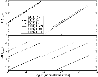
Figure 18: Same as Fig. 16, but for different values of $(\Gamma_{\mathrm{R}},\Delta g,\log\sigma)$.

References

- (1) Aloy, M.-A., Ibáñez, J.M., Martí, J.M., M’́uller, E. 1999, ApJSupl. Ser., 122, 151
- (2) Brinkmann W., Sembay S., Griffiths R.G., et al. 2001, A&A, 365, L162
- (3) Brinkmann W., Papadakis, I.E., den Herder, J.W.A., & Haberl F. 2003, A&A, 402, 929
- (4) Brinkmann W., Papadakis I. E., Raeth C., Mimica P., & Haberl F. 2005, A&A, 443, 397
- (5) Daigne, F., Mochkovitch, R., 1998, MNRAS, 196, 275
- (6) Fan, Y. Z., Wei, D. M., Zhang, B., 2004, MNRAS 354, 1031
- (7) Fossati G., Maraschi L., Celotti A., Comastri A., Ghisellini G., 1998, MNRAS 299, 433
- (8) Ghirlanda G., Ghisellini G., Celotti A., 2004, A&A, 422, 55
- (9) Ghisellini G., Celotti A., Fossati G., Maraschi L., Comastri A.,1998, MNRAS 301, 451
- (10) Janka H.-Th., Aloy M.-A., Mazzali P. A., Pian E., 2006 ApJ, 645, 1305
- (11) Kino M., Mizuta A., & Yamada S. 2004, ApJ, 611, 1021
- (12) Leismann, T., Antón, L., Aloy, M. A., Müller, E., Martí, J. M., Miralles, J. A., Ibáñez, J. M. 2005, A&A, 436, 503
- (13) Maraschi, L., Fossati G., Tavecchio F., et al. 1999, ApJ, 526, L81
- (14) Mimica P., Aloy M.-A., Müller E., Brinkmann W. 2004, A&A, 418, 947
- (15) Mimica P., Aloy M.-A., Müller E., Brinkmann W. 2005, A&A, 441, 103
- (16) Ravasio, M., Tagliaferri, G., Ghisellini, G., Tavecchio, F. 2004, A&A, 424, 841
- (17) Rees M.J., Mészáros P. 1994, ApJL, 430, 93
- (18) Romero R., Martí J.M., Pons J.A., Ibáñez J.M., Miralles J.A. 2005, J. Fluid Mech., 544, 323
- (19) Sari, R., & Piran, T. 1995, ApJ, 455, L133
- (20) Sari, R., & Piran, T. 1997, ApJ, 485, 270
- (21) Spada, M., Ghisellini G., Lazzatti D., & Celotti, A. 2001, MNRAS, 325, 1559
- (22) Takahashi T., Kataoka J., Madejski G., et al. 2000, ApJ, 542, L105
- (23) Zhang, Y.H., Treves, A., Maraschi, L., Bai, G.M. Liu, F.K., 2006, ApJ, 637, 699
- (24) Zhang, B., Kobayashi S. 2005, ApJ, 628, 315