Using the cluster mass function from weak lensing to constrain neutrino masses

Abstract

We discuss the variation of cosmological upper bounds on $M_{\nu}$, the sum of the neutrino masses, with the choice of data sets included in the analysis, pointing out a few oddities not easily seen when all data sets are combined. For example, the effect of applying different priors varies significantly depending on whether we use the power spectrum from the 2dFGRS or SDSS galaxy survey. A conservative neutrino mass limit of $M_{\nu}<1.43$eV (95%C.L.) is obtained by combining the WMAP 3 year data with the cluster mass function measured by weak gravitational lensing. This limit has the virtue of not making any assumptions about the bias of luminous matter with respect to the dark matter, and is in this sense (and this sense only) bias-free.

I Introduction

The fact that neutrinos undergo flavour oscillations, implying that not all neutrinos are massless, is one of the most important discoveries in particle physics in the last decade. Oscillations are only sensitive to the mass-squared differences between the neutrino mass eigenstates (see e.g. Maltoni et al. (2004); Fogli et al. (2006)), and although these are suggestive of the overall mass scale, they cannot pin the absolute mass scale firmly. For that, one needs probes like tritium beta decay Eitel (2005) or neutrinoless double beta decay Elliott and Vogel (2002). At the moment, however, the strongest upper bound on the neutrino mass scale comes from cosmology (see e.g. Goobar et al. (2006); Seljak et al. (2006)). The cosmological mass limits are based on the implications of neutrino masses for clustering of matter, in particular the fact that neutrinos can free-stream out of density perturbations and impede structure formation on small scales if they are a significant fraction of the dark matter. For a thorough review, see Lesgourgues and Pastor (2006).

Impressive as they are, the cosmological neutrino mass limits involve several assumptions. First of all, they assume that the underlying cosmological model is of the Friedmann-Robertson-Walker type, that gravity is described by general relativity, the primordial power spectrum of density perturbations is a scale-free power-law, and that the dark energy is a cosmological constant. Modifications of this simple picture have been considered Zunckel and Ferreira (2006), and in particular the degeneracy between neutrino masses and the dark energy equation of state has been investigated in some recent papers Hannestad (2005); Goobar et al. (2006); Ichikawa and Takahashi (2005); De La Macorra et al. (2006); Xia et al. (2006). Secondly, the upper limit depends on the cosmological data sets used in the analysis. It is this last aspect of the problem we will consider in the present paper, working within the context of the standard $\Lambda$CDM paradigm.

The angular power spectrum of the temperature anisotropies in the cosmic microwave background (CMB) radiation is generally considered to be the cleanest cosmological data set. Unfortunately the CMB temperature power spectrum cannot provide upper limits on $M_{\nu}$ better than $\sim 1.6$ eV Ichikawa et al. (2005), which is almost reached already now with the WMAP 3-year data Spergel et al. (2006); Fukugita et al. (2006); Kristiansen et al. (2006). An improvement of this limit requires some probe of the matter distribution. The most common probe is the power spectrum of the galaxy distribution, as determined by large redshift surveys like the 2 degree Field Galaxy Redshift Survey (2dFGRS) Cole et al. (2005) and the Sloan Digital Sky Survey (SDSS) Tegmark et al. (2004a). The distribution of the galaxies is biased with respect to that of the dark matter, but if the bias is independent of length scale, this is not a serious limitation. However, recent results suggest that the story of bias might be more complicated than the simple assumption of scale-independent bias that has gone into earlier cosmological mass limits Percival et al. (2006); Smith et al. (2006).

Ideally, one would like to rely on probes that are sensitive to the total matter distribution. One such probe is measurements of weak gravitational lensing by matter along random lines of sight Refregier (2003); Schneider (2006). However, even the most ambitious of these ’cosmic shear’ surveys have covered less than one percent of the full sky, thus probing only a limited cosmological volume. A somewhat different approach is to count the number of rare, high density peaks in the matter fluctuations within a larger volume. These peaks correspond to very massive clusters of galaxies, their abundances (the so-called cluster mass function) being highly sensitive to the amplitude of the matter power spectrum (see e.g. Voit (2005) and references therein) on corresponding scales. Until recently, cluster masses were generally derived based on observables of the baryonic mass component, such as the temperature of the X-ray emitting intra-cluster medium (ICM). In this case, one had to calibrate the X-ray temperature-mass relationship, either from simulations or from observational mass measurements relying on assumptions about hydrostatical equilibrium of the ICM. However, Dahle Dahle (2006) provided for the first time a measurement of the cluster mass function (CMF) where the cluster masses have been established directly by weak gravitational lensing. The main result of this paper is an upper bound on the sum of the neutrino masses obtained by combining the WMAP 3-year data with the CMF derived by Dahle Dahle (2006). Although not as impressive as e.g. the limit obtained by combining all available cosmological observations, including the Lyman alpha forest power spectrum (see e.g. Seljak et al. (2006); Cirelli and Strumia (2006)), this limit is robust in the sense that it makes use of clean cosmological probes, and involves a minimum of assumptions.

II Massive neutrinos in cosmology

We work within the standard cosmological paradigm of the $\Lambda$CDM model, and leave studies of significant deviations from this model for a future study. Our adopted notation is as follows: We denote as $\Omega_{\rm i}$ the present density of component ${\rm i}$ in units of the density of a spatially flat universe. Note that $\Omega_{\rm m}$ is the total density of all non-relativistic components, so that $\Omega_{\rm m}=\Omega_{\rm{CDM}}+\Omega_{\rm b}+\Omega_{\nu}$, with $\Omega_{\rm b}$ being the present baryon density. The density parameter $\Omega_{\nu}$ is determined by the sum of the neutrino masses $M_{\nu}$ and the present value of the Hubble parameter $H_{0}=100h\;{\rm km}\,{\rm s}^{-1}\,{\rm Mpc}^{-1}$ Mangano et al. (2005):

$$\Omega_{\nu}h^{2}=\frac{M_{\nu}}{93.14\;{\rm eV}}.$$ (1)

As we will see, present cosmological probes (with the possible exception of the Lyman alpha forest Seljak et al. (2006)) are only sensitive to neutrino masses larger than a few tenths of an eV. In this regime, the neutrino mass spectrum would be degenerate, and hence $M_{\nu}=3m_{\nu}$, where $m_{\nu}$ is the common mass of the neutrino mass eigenstates.

Within the $\Lambda$CDM model the effect of massive neutrinos on structure formation is simple. Their influence on structure formation is governed mainly by the quantity $f_{\nu}=\Omega_{\nu}/\Omega_{\rm m}$. While relativistic, the neutrinos free-stream out of density perturbations on scales smaller than the Hubble radius. Once they become non-relativistic, the free-streaming scale is set by their root-mean-square velocity. The maximum length scale below which all scales are affected by neutrino free-streaming is thus set by the horizon size when the neutrinos became non-relativistic. This quantity is given by Lesgourgues and Pastor (2006)

$$k_{\rm nr} = 0.018\left(\frac{m_{\nu}}{1\;{\rm eV}}\right)^{1/2}\Omega_{\rm m}^{1/2}\;h\,{\rm Mpc}^{-1}$$ (2)

$$= 0.1f_{\nu}^{1/2}\Omega_{\rm m}h\;h\,{\rm Mpc}^{-1}.$$

Note that the combination $\Omega_{\rm m}h$ enters this expression; this quantity determines the Hubble radius at matter-radiation equality and is an important length scale in the power spectrum of matter density fluctuations. This scale is similar to the neutrino free-streaming scale: below this scale, density perturbations are suppressed. Hence, there is a degeneracy between $\Omega_{\rm m}h$ and $f_{\nu}$.

For scales below the neutrino free-streaming scale, $k>k_{\rm nr}$, the main effect is a reduction by a factor $1-f_{\nu}$ of the source term in the equation for the linear growth of density perturbation. Hence, the amount of suppression is also set by the parameter $f_{\nu}$, and so it is this, and not $M_{\nu}$ which is directly accessible in measurements of large-scale structure. Since we can write $M_{\nu}=93.14f_{\nu}\Omega_{\rm m}h^{2}\;{\rm eV}$, we see that one also needs a constraint on $\Omega_{\rm m}h^{2}$ to go from a limit on $f_{\nu}$ to a limit on $M_{\nu}$. Figure 1 illustrates this situation in a toy example. It is seen that the matter power spectrum must be combined with other probes, for example the CMB power spectrum, in order to provide stringent constraints on $M_{\nu}$.

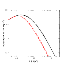
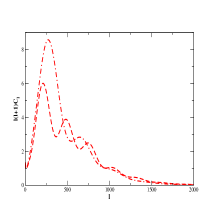
Figure 1: Illustration of how combining data sets break degeneracies. The left panel shows the matter power spectrum in four different models, where the baryon density has been artificially set low and a scale invariant power spectrum of adiabatic primordial perturbations has been assumed. The black lines are for models with $\Omega_{\nu}=0$. The full line has $\Omega_{\rm m}=0.25$ and $h=0.735$, whereas the dotted line has $\Omega_{\rm m}=0.50$ and $h=0.3675$. The red lines are models with massive neutrinos. The dashed line has $\Omega_{\rm m}=0.25$, $\Omega_{\nu}=0.05$ and $h=0.735$, and the dot-dashed line has $\Omega_{\rm m}=0.50$, $\Omega_{\nu}=0.10$ and $h=0.3675$. Note that $f_{\nu}=0.2$ in both cases. The right panel shows the CMB power spectra for the two models with massive neutrinos, with the same line coding. The models have very different CMB power spectra, and hence measurements of the CMB anisotropies help constraining $\Omega_{\nu}$.

III Data and methods

In our analysis we have used data from both CMB, observations of large scale structures (LSS), type Ia supernovae (SNIa), baryon acoustic oscillations (BAO), and additional priors on the Hubble parameter and the baryon content of the universe. We have also applied constraints on the cluster mass function from weak gravitational lensing.

III.1 CMB data

The 3-year data release from the WMAP team Hinshaw et al. (2006) is at present the most constraining set of CMB observations. The WMAP experiment is a full-sky survey of CMB temperature anisotropies. With this release, a Fortran 90 code for calculating the likelihood of a given CMB power spectrum against the data was also provided. However, in ref. Eriksen et al. (2006) it was noted that this likelihood code applied a sub-optimal likelihood approximation on large scales ($l\lesssim 30$), and in ref. Huffenberger et al. (2006) the authors pointed out an over-subtraction of unresolved point sources on small angular scales ($l\gtrsim 30$). Correcting for these two effects resulted in a slight shift in some cosmological parameter values. In ref. Kristiansen et al. (2006), it was shown that these corrections to the WMAP likelihood code also shifted the upper limit on the neutrino masses from $M_{\nu}<1.90$eV to $M_{\nu}<1.57$eV when using WMAP data only. In a revised version of the WMAP likelihood code, these corrections have to some extent been accounted for, and the results using this code is in better agreement with refs. Huffenberger et al. (2006); Kristiansen et al. (2006) than the previous version. In this paper we will make use of this revised likelihood code from the WMAP team. We note, however, that the upper limits on $M_{\nu}$ would have been slightly lower with the code used in refs. Huffenberger et al. (2006); Kristiansen et al. (2006).

In this work we are not considering CMB data from other experiments than WMAP, since we want to restrict the number of data sets as much as possible, and since these additional data sets have been shown not to improve the limits on $M_{\nu}$ Kristiansen et al. (2006).

III.2 Large scale structure

Large scale structure surveys probe the matter distribution in the universe by measuring the galaxy-galaxy power spectrum $P_{g}(k,z)=\langle|\delta_{g}(k,z)|^{2}\rangle$. Since massive neutrinos give a distinct imprint on the LSS due to their free-streaming effect, data from galaxy surveys have proven to be important to put tight constraints on neutrino masses. However, such surveys are also troubled by bias effects that are hard to quantify. For example, it is assumed that in the linear perturbation regime, the total matter power spectrum, $P_{m}$, is proportional to the galaxy power spectrum by the simple relation $P_{g}=b^{2}P_{m}$. Recently, the use of this simple relation has been debated Percival et al. (2006); Smith et al. (2006), and it is at present unclear what the precise corrections from a scale-dependent $b$ might be.

There are two galaxy surveys of comparable size, the 2 degree Field Galaxy Redshift Survey (2dFGRS) Cole et al. (2005), and the Sloan Digital Sky Survey (SDSS) main sample Tegmark et al. (2004b). As has been pointed out in e.g. Sanchez et al. (2006); Percival et al. (2006); Cole et al. (2006), there seems to be some tension between the results from 2dFGRS and SDSS. As a relevant example for this paper, the combination SDSS+WMAP prefers larger values of both $\Omega_{\rm m}$ and $\sigma_{8}$ (the rms mass fluctuations in spheres of radius $8h^{-1}$ Mpc) than what is found when using data from 2dFGRS+WMAP. In a recent analysis of the 2dFGRS-SDSS discrepancy Cole et al. (2006), the authors conclude that it is caused by non-linear bias effects. They also claim that SDSS is more sensitive to these effects than the 2dFGRS sample, since the SDSS sample contains more red galaxies, which are believed to cluster slightly different from blue galaxies.

Regardless of their origin, the reported inconsistencies between the 2dFGRS and SDSS galaxy surveys tell us that we should always be cautious when including LSS data in our parameter estimation, at least until the scale dependence of the bias parameter is better understood.

When including 2dFGRS and SDSS data in our analysis we have tried to use as commonly used analysis techniques as possible. We have therefore stuck to the default analysis and parameter choices in the CosmoMC code. For the 2dFGRS data this implies discarding all scales with $k>0.15h\textrm{Mpc}^{-1}$. This corresponds to the choice made in e.g. Sanchez et al. (2006). For the 2dFGRS data we also use the prescribed correction for nonlinearities given in Cole et al. (2005), $P_{g}=(1+Qk^{2})/(1+Ak)$ with $A=1.4$ and $Q=4.0\pm 1.5$. For SDSS we discard scales with $k>0.20h\textrm{Mpc}^{-1}$, as is done in e.g. Tegmark et al. (2004a). In this paper they find that using this cutoff scale yields results that are consistent with the what they find when applying more a more conservative cutoff on $k$. No corrections for non-linearities are included in our SDSS analysis. The treatment of cutoffs and nonlinearities in the analysis of the 2dFGRS and SDSS data are different. Thus, if any tension is found between these two data sets here, it is not obvious whether this stems from problems within the datasets or if it is caused by the way the data sets are analysed here. However, any such tension would illustrate that there are problems related to using LSS surveys for parameter estimation when adapting these commonly used analysis methods for the two surveys.

III.3 Type Ia supernovae

The luminosity distance-redshift relationship measured by observations of supernovae of type Ia (SNIa) provides the most direct evidence for cosmic acceleration and dark energy. There are still open questions regarding both the exact mechanism behind these supernovae and their use as ‘standard candles’, and so we choose not to rely on SNIa in our robust neutrino mass limit. When we do use them, we use the data from the Supernova Legacy Survey (SNLS) Astier et al. (2006).

III.4 The cluster mass function

Massive galaxy clusters are extremely rare high-density peaks in the matter fluctuations, containing matter originating from a co-moving volume spanning $\sim 10h^{-1}$ Mpc which has undergone gravitational collapse. Their abundances, as quantified by the CMF, are thus a sensitive probe of $\sigma_{8}$ and $\Omega_{\rm m}$. While all previous measurements of the CMF have been based on observations of baryonic tracers of cluster mass (with inherent uncertainties and possible biases which are not yet fully understood; see e.g. Rasia et al. (2006)), the CMF of Dahle (2006) was derived from weak gravitational lensing measurements of the masses of a volume-limited sample of X-ray luminous clusters. The details of the data reduction and weak gravitational shear estimator are given in Dahle et al. (2002), and Dahle (2006) describes the derivation of cluster masses from gravitational lensing measurements. The cluster sample of Dahle (2006) was selected from a large volume of $8.0\times 10^{8}(h^{-1}{\rm Mpc})^{3}$ (assuming a spatially flat universe with $\Omega_{\rm m}=0.3$), above a threshold value in X-ray luminosity ($L_{\rm X}$). Using $L_{\rm X}$ as a proxy for mass in the cluster selection could in principle introduce a baryonic bias to the CMF measurements, depending on $L_{\rm X}$ measurement uncertainties and the intrinsic scatter around the mass-$L_{\rm X}$ relation. In Dahle (2006), any such effects were effectively removed, by carefully calibrating the amplitude of the mass-$L_{\rm X}$ relation and the scatter around the mean relation (thereby estimating the sample completeness as a function of mass), and by calculating cosmological parameter constraints exclusively based on the clusters well above the mass threshold corresponding to the X-ray luminosity threshold of the sample (where the sample is virtually complete). Other statistical and systematic uncertainties in the derived cluster masses and the effects of these uncertainties on the CMF constraints are discussed in detail in Dahle (2006).

Parameter constraints in the $\sigma_{8}-\Omega_{\rm m}$ plane were obtained by fitting the observed cluster abundances in three mass intervals to theoretical predictions for the CMF Sheth and Tormen (1999).

We have found that the value of $\chi^{2}$ from the CMF from Dahle (2006) can be approximated by the fit-function

$$\chi^{2}_{\textrm{CMF}}=10000u^{4}+6726u^{3}+1230u^{2}-4.09u+0.004,$$ (3)

where $u=\sigma_{8}(\Omega_{\rm m}/0.3)^{0.37}-0.67$. This result is rather insensitive to the choice of theoretical mass function: As noted by Dahle (2006), replacing the CMF prediction used here Sheth and Tormen (1999) with a more recent predicted CMF based on N-body simulations Warren et al. (2006) (taking into account the differing mass definitions in these two works) only results in a shift of 0.01 in $u$.

III.5 Other priors

We have also tested the sensitivity of neutrino mass limits on priors from the Hubble Space Telescope Key Project on the Extragalactic Distance Scale (HST), and Big Bang nucleosyntesis (BBN) predictions.

From HST, we use a prior on the Hubble parameter of $h=0.72\pm 0.08$ Freedman et al. (2001), and from BBN we use a prior on the physical baryon density today, $\Omega_{b}h^{2}=0.022\pm 0.002$ Burles et al. (2001); Cyburt (2004); Serpico et al. (2004). There are hints of some tension between the WMAP constraint on $\Omega_{\rm b}h^{2}$ and the value of this quantity inferred from the ${}^{4}{\rm He}$ abundance Steigman (2006), so in our robust limit we will not use the BBN prior. Since there is still some debate about the value of the Hubble constant derived from the HST Key Project Blanchard et al. (2003); Sandage et al. (2006), we also drop this prior when deriving our robust limit.

We have also added information on the position of the baryonic acoustic oscillation (BAO) peak in the luminous red galaxy (LRG) sample in the SDSS survey Eisenstein et al. (2005). This prior is implemented by an effective fit function as described in Goobar et al. (2006). Using an effective parameter

$$A_{\textrm{BAO}}=\left[D_{M}(z)^{2}\frac{z}{H(z)}\right]^{1/3}\frac{\sqrt{\Omega_{\rm m}H_{0}^{2}}}{z},$$ (4)

where $D_{M}(z)$ is the comoving angular diameter distance, the authors impose the constraint

$$A_{\textrm{BAO}}=0.469\left(\frac{n_{s}}{0.98}\right)^{-0.35}(1+0.94f_{\nu})\pm 0.017.$$ (5)

Throughout our analysis we have also applied a top-hat prior on the age of the universe, $10\textrm{Gyr}<\textrm{Age}<20\textrm{Gyr}$.

III.6 Parameter estimation

For the parameter estimations we have used the publicly available Markov chain Monte Carlo code CosmoMC Lewis and Bridle (2002). We have used a basic seven-parameter model, varying the parameters $\{\Omega_{b}h^{2},\Omega_{\rm m},\log{(10^{10}A_{S})},h,n_{s},\tau,M_{\nu}\}$. $M_{\nu}$ is defined in eq. (1). For the other parameters, the exact definitions are given by the CosmoMC code. We have assumed spatial flatness, no running of the scalar spectral index, that the dark energy is a cosmological constant and that the tensor to scalar fluctuation amplitude is negligible. These assumptions are well motivated by current available data Spergel et al. (2006). Also, adding these extra degrees of freedom do not affect the limits on $M_{\nu}$ drastically Kristiansen et al. (2006).

Often cosmological neutrino mass limits are found using a large number of different data sets and priors simultaneously. In this analysis we consider in total 48 different combinations of data sets and priors to see how the different data sets alter the neutrino mass limit.

IV Results

The neutrino mass limits found in our analysis are summarized in Table 1. The limits quoted in the table range from $M_{\nu}\lesssim 6$eV from using LSS data only, via $M_{\nu}<1.75$eV from WMAP data only, and down to $M_{\nu}<0.40$eV for a combination of WMAP, SDSS, SNLS BAO and HST data.

Data set	no prior	CMF	HST	BBN
WMAP	1.75eV	1.43eV	1.47eV	1.73eV
WMAP+2dFGRS	1.02eV	0.89eV	0.92eV	1.01eV
WMAP+SDSS	1.05eV	1.13eV	0.87eV	1.05eV
WMAP+SNLS	1.10eV	0.70eV	1.02eV	1.07eV
SDSS	5.8eV	4.6eV	6.1eV	6.0eV
2dFGRS	5.2eV	5.3eV	5.3eV	5.2eV
WMAP+2dFGRS+SNLS	0.81eV	0.64eV	0.76eV	0.80eV
WMAP+SDSS+SNLS	0.44eV	0.57eV	0.42eV	0.44eV
WMAP+2dFGRS+SNLS+BAO	0.84eV	0.69eV	0.79eV	0.84eV
WMAP+SDSS+SNLS+BAO	0.42eV	0.56eV	0.40eV	0.42eV
WMAP+SDSS+BAO	0.55eV	0.76eV	0.52eV	0.56eV
WMAP+2dFGRS+BAO	1.04eV	0.89eV	0.92eV	1.01eV

Table 1: Estimated 95% C.L. upper limits on $M_{\nu}$. The CMF, HST and BBN priors are added one at the time to the combination of data sets given in the left column.

IV.1 WMAP + priors

As one might have expected, the inclusion of WMAP data is crucial for finding a good neutrino mass limit. The upper limit from WMAP data alone found here, $M_{\nu}<1.75$eV, resides between the former results found by the WMAP team for their 3 year data, $M_{\nu}<2.0$eV Spergel et al. (2006), and the results from ref. Kristiansen et al. (2006) using the same data with a modified likelihood code, $M_{\nu}<1.57$eV. In this case we see that both a CMF and HST prior will help significantly in constraining $M_{\nu}$, and adding the CMF prior to the WMAP data yields an upper bound of $M_{\nu}<1.43$eV.

The CMF prior put constraints on a combination of $\Omega_{\rm m}$ and $\sigma_{8}$, and in Figure 2 we show confidence contours in the plane of $M_{\nu}$ and $\sigma_{8}(\Omega_{\rm m}/0.3)^{0.37}$ from WMAP data only, and when we add the CMF prior. It is well known that there is a positive correlation between $M_{\nu}$ and $\Omega_{\rm m}$ in the CMB power spectrum. Both these parameters will alter the amplitudes of the CMB peaks, by shifting the time of matter-radiation equality. At this time neutrinos in this mass range were still relativistic, and contributed to the radiation part. Keeping $\Omega_{\rm m}$ constant and increasing $f_{\nu}$ will thus postpone the time of matter-radiation equality and therefore enhance the amplitude of the acoustic peaks. To shift the time of equality back and lower the acoustic peaks, one has to increase $\Omega_{\rm m}$ correspondingly. However, the effective parameter from the CMF constraint, $\sigma_{8}(\Omega_{\rm m}/0.3)^{0.37}$, also contains the amplitude parameter $\sigma_{8}$ which is negatively correlated with $M_{\nu}$ (from the same reasoning). From Figure 2 we see that this negative correlation is strong enough to make also the correlation between $M_{\nu}$ and $\sigma_{8}(\Omega_{\rm m}/0.3)^{0.37}$ negative; that is, small values of $\sigma_{8}(\Omega_{\rm m}/0.3)^{0.37}$ favor a large neutrino mass. When we add the CMF prior the allowed region of low values of $\sigma_{8}(\Omega_{\rm m}/0.3)^{0.37}$ shrinks, and the upper limit on $M_{\nu}$ is reduced correspondingly.

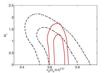
Figure 2: 68% and 95% C.L. contours in the plane of $M_{\nu}$ and the effective parameter from the CMF constraint, $\sigma_{8}(\Omega_{\rm m}/0.3)^{0.37}$. The dashed black line shows the contours when using WMAP data only, and the solid black lines show the results when adding the prior from the CMF.

Note that with this limit ($M_{\nu}<1.43$eV) we have not used any LSS or SNIa data, or any other prior on $H_{0}$ or $\Omega_{b}$. We therefore claim this neutrino mass limit to be robust.

IV.2 Including large scale structure

When adding LSS data the neutrino mass limit improves significantly, giving $M_{\nu}<1.02$eV for WMAP+2dFGRS and $M_{\nu}<1.05$eV for WMAP +SDSS. However, when adding the CMF prior, a strange effect occurs. While this improves the $M_{\nu}$ limit to $M_{\nu}<0.89$eV in the case of WMAP+2dFGRS, the limit increases to $M_{\nu}<1.13$eV with WMAP+SDSS. This may indicate a inconsistency between the CMF prior and our SDSS analysis. In Figure 3 we show the marginalized distribution of the $\sigma_{8}(\Omega_{\rm m}/0.3)^{0.37}$ parameter when using WMAP, WMAP+CMF, WMAP+2dFGRS, WMAP+SNLS or WMAP+SDSS. For the latter, the distribution deviates significantly from the four former, and we see that the WMAP+SDSS data set prefers larger values of $\sigma_{8}(\Omega_{\rm m}/0.3)^{0.37}$ than than the other combinations. This is in good accordance with the results obtained in ref. Sanchez et al. (2006), where they found that WMAP+SDSS preferred larger values for both $\Omega_{\rm m}$ and $\sigma_{8}$ than what was found with WMAP alone or WMAP+2dFGRS (using the WMAP 1-year data). Figure 3 indicates that we should be careful when using data from SDSS in combination with 2dFGRS or CMF. Doing this, the inconsistencies may produce artificially narrow parameter distributions. In our case, the result of using WMAP+SDSS+CMF is that we not only get an upper limit on $M_{\nu}$, but also a lower limit, such that our 95% C.L. limit becomes $0.23\textrm{eV}<M_{\nu}<1.13$eV for this combination of data sets. In Figure 4 we show the confidence contours in the plane of $\sigma_{8}(\Omega_{\rm m}/0.3)^{0.37}$ and $M_{\nu}$ for WMAP+2dFGRS and WMAP+SDSS with and without the CMF prior. From these plots it is clear how the incompatibility of SDSS and CMF produces the lower limit on $M_{\nu}$.

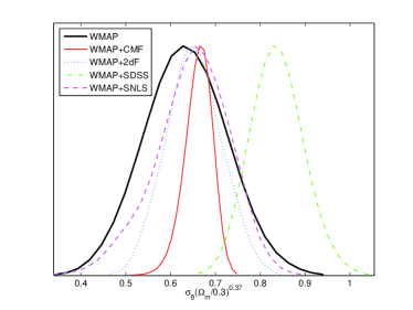
Figure 3: Marginalized one-dimensional distribution of $\sigma_{8}\left(\Omega_{\rm m}/0.3\right)^{0.37}$ when using WMAP data (thick black line), WMAP+CMF (solid red line), WMAP+2dFGRS (dotted blue line), WMAP+SDSS (dash-dotted green line) and WMAP+SNLS (dashed purple line).

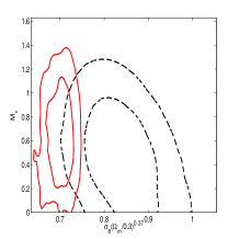
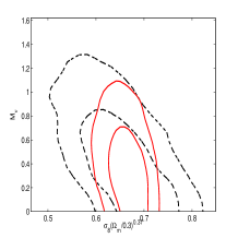
Figure 4: 68% and 95% C.L. contours in the plane of $\sigma_{8}(\Omega_{\rm m}/0.3)^{0.37}$ and $M_{\nu}$. Left panel: Contours from WMAP+SDSS (black, dashed line), and WMAP+SDSS+CMF (red, solid line). Right panel: Contours from WMAP+2dFGRS (black, dashed line), and WMAP+2dFGRS+CMF (red, solid line).

When adding LSS data to the WMAP data set, we see that the HST prior is still important to improve the $M_{\nu}$ limits, while the BBN prior is not needed.

Also, it is interesting to note that adding the BAO prior to the WMAP+2dFGRS data set combination has essentially no effect for the neutrino mass limits, whereas adding the BAO prior to the WMAP+SDSS data sets improves the neutrino mass limit by almost a factor two. Again this illustrates the differences between the 2dFGRS and SDSS sample in our analysis. The reason why the BAO prior is more important when using SDSS, is the larger preferred value of $\Omega_{\rm m}h^{2}$ for the SDSS sample. Adding the BAO prior will constrain the allowed region of large $\Omega_{\rm m}h^{2}$, and thus also the allowed space for large $M_{\nu}$.

We have also tried to constrain $M_{\nu}$ using LSS data alone, resulting in mass limits of order $M_{\nu}\lesssim 6$eV. So although LSS data in principle is a sensitive probe for neutrino masses, one needs to add CMB data to break parameter degeneracies.

IV.3 Including supernova data

The inclusion of supernova data turns out to be as important as LSS for constraining neutrino masses. Again, this can be understood by the $M_{\nu}$-$\Omega_{\rm m}$ degeneracy. SNIa data is an effective probe of the amount of dark energy in the universe, and under the flatness assumption this will also automatically constrain $\Omega_{\rm m}$. In Figure 3 we see that also the data set combination WMAP+SNLS seems to be consistent with WMAP alone, WMAP+2dFGRS and CMF prior, whereas it seems to be in some tension with our SDSS analysis. In the case of WMAP+SNLS we see from Table 1 that adding the CMF prior improves the neutrino mass limit significantly, and that the inclusion of the CMF prior is a lot more constraining for neutrino masses than both the HST and BBN prior in this case. This means that if one believes in the SNIa measurements, we have an upper limit of $M_{\nu}<0.70$eV without using LSS measurements at all.

Note also that we can get a neutrino mass limit as low as $M_{\nu}<0.40$eV without using Ly-$\alpha$ data, if we combine WMAP+SNLS+SDSS+BAO+HST. But this limit weakens to $M_{\nu}<0.79$eV by substituting SDSS with 2dFGRS. Again, this illustrates how sensitive the neutrino mass limit is to the choice of LSS sample and combination of priors.

V Conclusion

In this paper we have studied cosmological neutrino mass limits, and how sensitive these limits are to different choices of data sets and priors. We have also included a new prior from the cluster mass function measured by weak gravitational lensing, which is a direct probe of the total mass distribution in the universe.

We report neutrino mass limits using 48 different combinations of data sets and priors, and we find that the neutrino mass limit is very sensitive to small changes in combinations of data sets and priors. Especially striking results are found when interchanging data sets between the SDSS and 2dFGRS galaxy surveys. For example will the combination WMAP+SDSS+BAO give $M_{\nu}<0.52$eV at 95% C.L., while WMAP+2dFGRS+BAO gives $M_{\nu}<0.97$eV. These discrepancies occur because of a slight inconsistency between the SDSS data as analysed here and many of the other data sets used. Combining inconsistent data sets may of course lead to unreliable results. Also, the tension between the two galaxy surveys indicate that there may be systematics related to e.g. the scale dependence of the bias parameter that have to be better understood before we can rely fully on the LSS analysis. By discarding these data sets, and in addition refraining from using constraints from SNIa, HST, and BBN, we end up with a conservative, although robust cosmological neutrino mass limit of $M_{\nu}<1.43$eV from using only WMAP data in combination with the CMF prior.