Velocities measured in small scale solar magnetic elements.

Abstract

We have obtained high resolution spectrograms of small scale magnetic structures with the Swedish 1-m Solar Telescope. We present Doppler measurements at $0\farcs{2}$ spatial resolution of bright points, ribbons and flowers and their immediate surroundings, in the C I 5380.3 Å line (formed in the deep photosphere) and the two Fe I lines at 5379.6 Å and 5386.3 Å. The velocity inside the flowers and ribbons are measured to be almost zero, while we observe downflows at the edges. These downflows are increasing with decreasing height. We also analyze realistic magneto-convective simulations to obtain a better understanding of the interpretation of the observed signal. We calculate how the Doppler signal depends on the velocity field in various structures. Both the smearing effect of the non-negligible width of this velocity response function along the line of sight and of the smearing from the telescope and atmospheric point spread function are discussed. These studies lead us to the conclusion that the velocity inside the magnetic elements are really upflow of the order 1–2 km s^-1 while the downflows at the edges really are much stronger than observed, of the order 1.5–3.3 km s^-1.

1. Introduction

In the Sun’s photosphere one can observe magnetic structures in a range of different scales. From sunspots of tens of Mm size to small scale magnetic elements of about 200 km or less. Observationally these small scale magnetic elements become visible as features brighter than the surroundings (leading to the often used term “bright points”) when the photosphere is imaged at sufficiently high angular resolutions (Dunn & Zirker, 1973). Title & Berger (1996) showed that bright points can not be detected with spatial resolutions worse than about $0\farcs 4$ due to a smearing out of the contrast because bright points are surrounded by darker areas. As observational methods have become more sophisticated, such as adaptive optics (e.g. Rimmele, 2000; Scharmer et al., 2003b) and post-processing methods (e.g. von der Luehe, 1993; van Noort et al., 2005), the observations of such structures have become almost routine. Recently Berger et al. (2004) concluded that at 100 km resolution the magnetic elements do not always resolve into discrete bright elements. Instead, in plage regions of stronger average magnetic field, the small scale magnetic elements are found to be concentrated into elongated “ribbons” and round “flowers” with a darker core and bright edges. These elements are constantly evolving; the merging and splitting of “flux sheets” and the transitions between the ribbons, flowers, and micro-pores are described by Rouppe van der Voort et al. (2005). The understanding of these small scale elements is of great importance and these structures have therefore been subjected to intense research in recent years (e.g., Kiselman et al., 2001; Rutten et al., 2001; Sánchez Almeida et al., 2001; Steiner et al., 2001; Keller et al., 2004; Carlsson et al., 2004). This has resulted in good theoretical models and a good understanding of why the magnetic elements look the way they do in observations. One main conclusion of the above papers is that the dominant reason for the brightness of bright points is the lower density inside the bright point due to magnetic pressure, hence allowing the observer to look into deeper layers. These layers are hotter than the higher layers seen outside the magnetic elements because of the temperature increasing with depth. At equal geometric height, the temperature inside the magnetic element is lower than in the surroundings due to the suppression of convective energy transport by the magnetic field. This temperature contrast may be large enough in larger magnetic concentrations that it offsets the effect of the difference in formation height and the magnetic element no longer looks bright. Smaller magnetic elements (bright points) and the edges of the larger magnetic elements (ribbons, flowers, pores) are heated radiatively by the surrounding hotter, non-magnetic, atmosphere and we get a bright point or a bright edge. Bright points have often been observed in the G-band (spectral domain dominated by CH-molecular lines at 4300 Å). This is because bright points have higher contrast in this domain due to an increased height difference of the optical depth unity height because of the destruction of CH-molecules in low-density magnetic elements.

Rimmele (2004) presents measurements of the line of sight (LOS) velocity field in and around magnetic flux concentrations based on narrow-band filtergrams. He finds downdrafts at the edge of flux concentrations of “a few hundred meters per second.” The size of these downflow areas is approximately ${0\farcs 2}$, which indicates that they are smaller since this is the approximate spatial resolution of the observations. Furthermore he concludes that the downdraft gets narrower and stronger in deeper layers and the plasma within the flux concentration is more or less at rest. Rouppe van der Voort et al. (2005) found that magnetic structures such as flowers, ribbons and flux sheets have a weak upflow inside and a sharp downdraft at the edge in accordance with Rimmele (2004). The LOS flow inside flowers and ribbons was measured to be about 0–150 m s^-1 upflow and the downdrafts at the edge to about 360 m s^-1.

Both Rimmele (2004) and Rouppe van der Voort et al. (2005) use filtergrams at only two spectral positions to derive the velocities — adding more spectral sampling points would increase the accuracy of the measurements and would also make it possible to derive the velocity as a function of height. Spectroscopic measurements of bright points were reported by Langhans et al. (2002) and they derive velocity maps showing downflows close to bright points. Furthermore Langhans et al. (2004) use spectroscopic diagnostics to measure velocities inside bright points, at resolutions of about 0$\farcs$3 they find both upflows and downflows inside bright points.

In this paper, we present spectroscopic data of magnetic elements such as ribbons, flowers, and bright points with excellent spatial resolution. Intensity cuts of the smallest features and analysis of the spatial power spectrum show that the spatial resolution is better than 0$\farcs$2 for the spectra used in this work. These spectra are used to obtain the LOS velocities in and close to small scale magnetic elements. Furthermore we analyze a three dimensional simulation of magneto-convection by solving the radiative transfer through the simulation cube in the same spectral domain as in the observations. These simulations are used to understand the effects of the smearing along the line of sight (the velocity response function) and spatial smearing (the instrument and atmospheric point spread function(PSF)) have on the determinations of velocities.

In § 2 we present and discuss the observational program and the instrumentation. The data reduction methods are discussed in § 3. In § 4 we present the results of the Doppler shift measurements in the three spectral lines. The analysis of the Magneto-convective simulation, the determination of the velocity response functions in the diagnostics used, and the discussion of the smearing effects this kind of velocity measurements are hampered with are presented in § 5. Finally, we summarize our results in § 6.

2. Observing program and instrumentation

The main aim of these observations was to obtain good spectra in and close to small scale magnetic structures. On 2005 May 13 we observed the NOAA active region 10759 ($N8.4^{\circ}$, $E10.5^{\circ}$, $\mu=0.97$) using a small pore as adaptive optics lock point, see Fig.1 for an example of a slit-jaw image.

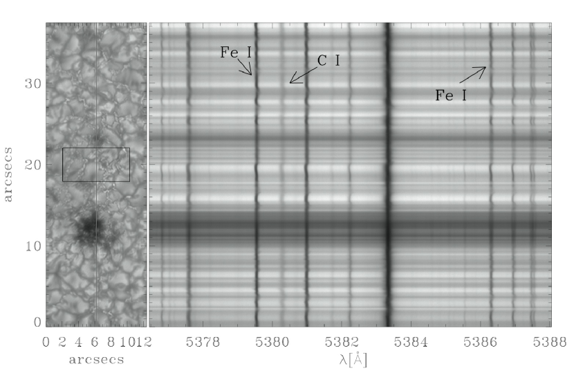
Figure 1.— Slit-jaw image (left) and the corresponding spectrogram (right). The slit-jaw image has been MFBD processed to facilitate the identification of small scale structures. The box in the slit-jaw image marks the area which has been magnified in Fig.3

The spectra were obtained using the Swedish 1-m Solar Telescope (SST) (Scharmer et al., 2003a) together with the adaptive optics system (Scharmer et al., 2003b) and the TRI-Port Polarimetric Echelle-Littrow (TRIPPEL) spectrograph. As indicated by the name, the TRIPPEL spectrograph is a Littrow spectrograph with an Echelle grating using 79 grooves mm^-1. The blaze angle is $63.43^{\circ}$, the focal length is $1500$ mm, and the slit width is $25~{}{\micron}$. Simultaneous spectra of two wavelength intervals, 4566–4576 Å (hereafter called the 4571 interval) and 5376.5–5388 Å (the 5380 interval), were obtained. In the present paper we focus on the 5380 interval since these spectra were obtained with the shortest exposure time and thus the Doppler shifts in the spectral lines will be less affected by seeing. The spectrograph should always be operated with angles close to the blaze angle. We observe at $62.73^{\circ}$ and in order 47 and 42 for the 4571 and 5380 intervals respectively. The theoretical slit-limited bandpass for the 5380 interval is $W_{\lambda}=23$ mÅ or in terms of effective theoretical spectral resolution $R\approx 234000$. In all our comparisons with FTS spectra and simulations we convolve these spectra to this resolution.

Two Megaplus 1.6 cameras (KAF-0401E Blue Plus and KAF-0401 Image sensor) were used at exposure times of 200 ms and 80 ms for the 4571 interval and 5380 interval respectively. The two cameras have a quantum efficiency of about $35\%$ and $25\%$ at the operating wavelengths. In addition to the spectral cameras we used two cameras to obtain slit-jaw images. One of the slit-jaw cameras using a 10.3 Å bandpass interference filter centered at 4572.6 Å was slaved to the spectral camera at the same wavelength. The other slit-jaw camera, using a 9.2 Å bandpass interference filter centered at 5321 Å, had exposure times of 8 ms and was not slaved. In the spatial domain the sampling is 0$\farcs$0411 pixel^-1. With this setup we observed several series of good to excellent seeing with a fixed slit-position. One of these series, with a duration of about 17 minutes (10:59:40–11:17:06 UT), is excellent both with respect to seeing conditions and structures crossed by the slit, see Fig.1. In the following all the data presented come from this series and we consider data of excellent quality spread over the full 17 minutes.

3. Data reduction

3.1. Flat fields and dark currents

The spectrograms are corrected for dark currents and flat fields. Flat fields are constructed from 5 series of 50 images of random scans of the quiet solar disk center. We then construct a mean spectrum. To obtain a mean spectrum we need to correct for the spectrograph’s main distortions, namely smile (the curvature of the spectral lines) and keystone (different spectral dispersion at different slit positions). The distortions are determined by fitting a 4th-order polynomial to the central part of the spectral line and in this way we measure the line core position over the slit. This is done for five lines distributed over the spectrogram. The smile is of order 4 pixels while the keystone is of order 0.15 pixels, thus the smile is the most profound aberration. The final flat fields are obtained by dividing the total of the 250 images by a distortion corrected mean spectrogram. In this way we remove both spatial and spectral information without losing the fixed CCD dependent signal and without any interpolation of pixels in the flat field.

3.2. Wavelength calibration

We make a mean solar spectrogram by adding together all 250 flat field spectra. The mean aberration corrected spectrum is then compared to the FTS atlas of Brault & Neckel (1987). This atlas has proved to be well calibrated in wavelength and it shows no systematic offset in line shifts with wavelength (Allende Prieto & Garcia Lopez, 1998). Since the solar atlas is corrected for the Earth’s rotation, the Earth’s orbital motion and the Sun’s rotation we automatically get a corrected spectrogram when we calibrate using the FTS atlas. The upper panel of Fig.2 gives a good impression of the accuracy of this calibration. Note that in this way our wavelength scale is the same as that of the FTS atlas; there is thus no correction for gravitational redshift. The slit covers a region of almost 38″ or approximately 28 Mm on the Sun. During the observations there is a temporal change of the spectral position on the cameras. This wavelength shift is the same in both spectral regions. Part of the shift is periodic, with an amplitude of 50–150 m s^-1 and a period of five minutes. This variation is caused by global oscillations averaged over the slit length. In addition there are slow trends, probably caused by temperature variations in the spectrograph. The frame to frame standard deviation is 8 m s^-1. We correct for this temporal change by applying a shift to the wavelength calibration determined form the flat field spectra. Since the slit is covering an active region, the mean spectrum of each slit is not directly comparable to the solar atlas (Brandt & Solanki, 1990, and references therein). Brandt & Solanki (1990) measure the mean convective blueshift in 19 Fe I lines, including the Fe I 5379 Å line, in quiet Sun and magnetically active regions. They find that the convective blueshifts are decreased from 350 m s^-1 in quiet Sun to 120 m s^-1 in active areas. We determine the temporal shifts by comparing the line center of the mean Fe I 5379 Å line in each spectrogram (averaged over an active region) with the line center position of the quiet Sun atlas. We thus need to compensate for the difference in line center convective blueshift between active regions and the quiet Sun. The difference of 230 m s^-1 found by Brandt & Solanki (1990) refers to an intensity level of 60% and not line center. From our observations we find that the difference is 30 m s^-1 smaller at line center. We thus apply a redshift of 200 m s^-1 to the atlas before comparing with our mean Fe I 5379 Å line when determining the temporal shift.

Figure 2.— Upper: FTS atlas of the Fe I 5379.6 Å line (solid) and the mean spectrum (dashed-dotted). The scattered light corrected mean spectrum is showed with triangles. Lower: Intensity level (intensity relative to the mean continuum intensity) of our quiet Sun spectrum (mean flat field spectrum) versus the intensity level of the FTS atlas (crosses) and a least-square linear fit to these data (solid).

Instead of correcting each spectrum for smile and keystone we use the determined aberrations to determine a separate wavelength scale for each slit position. This procedure avoids interpolation of the spectrogram data.

3.3. Scattered light

When the mean quiet Sun spectrum is plotted against the FTS atlas, see Fig.2 upper panel, it is clear that the mean spectrum has shallower lines than the FTS atlas. This discrepancy is due to scattered light, mainly from the diffuse scattering in the spectrograph. In the lower panel in Fig.2 we have plotted the intensity level of the mean spectrum against the FTS intensity level. We use a least-square linear fit to these data points. Assuming a constant level of diffuse scattered light, the offset and the new continuum calibration of the mean spectrum is given by this fit. The amount of constant scattered light is 6 %. This level is subtracted from the spectra and the resulting spectra are then divided by a scaling factor found from the slope of the curve in the lower panel of Fig.2. Again we refer to Fig.2 upper panel to see the effect of this correction of the scattered light.

According to Sobotka et al. (1994), “the mean intensity in abnormal granulation is equal to that of quiet granulation,” so we expect the mean spectrum from the flat fields to have the same mean count as we have in each of the mean spectrograms when we do not include the pores. This turns out not to be the case. There are many reasons for this discrepancy, different atmospheric conditions, the changing path length of the light ray in the atmosphere due to the time of the day and changing intensity on the Sun due to solar oscillations (p-modes). All these effects are corrected for by introducing a scaling factor which gives the same mean solar continuum intensity in the mean spectrum of each spectrogram as in the mean solar atlas. We multiply with this scaling factor before we correct for scattered light.

3.4. Slit-jaw images

The slit-jaw images are corrected for dark currents and flat fields and post-processed using the multi frame blind deconvolution (MFBD) method (van Noort et al., 2005). The intensity on the slit in the slit-jaw image is correlated to the mean intensity in the corresponding spectrogram to obtain the relative scaling and offset between the spectrogram and the slit-jaw image. The aligned slit-jaw images are used to identify the structures crossed by the slit, see Fig.1. Note that the slit-jaw image has shorter exposure time than the spectrum and has been post-processed — it is thus sharper and has a more narrow point-spread-function than the spectrogram.

4. Observed Doppler shifts

The 5380 interval contains the deep forming (Livingston et al., 1977) C I 5380.3 Å line, see Fig.1. Furthermore it contains a well suited quite strong Fe I line at 5379.6 Å and a weaker Fe I line at 5386.3 Å. These two iron lines have been singled out by other authors as good both in the sense that they are blend free and thus are well suited to measure the line asymmetry (Dravins et al., 1981) and that their central wavelengths are well known (Allende Prieto & Garcia Lopez, 1998). Nave et al. (1994) give the central wavelength of these Fe I lines, see Table 1, and they claim the error in the central wavelength of these two lines to be less than 1.25 mÅ and 2.5 mÅ respectively, which corresponds to uncertainties in velocities of 70 m s^-1 and 140 m s^-1. The central wavelength of the C I line is given by Johansson (1966) and he quotes the uncertainty to be less than 0.02 Å, which corresponds to 1115 m s^-1. This high uncertainty makes it difficult to use this line to determine velocities on an absolute scale. The Fe I line at 5383.3 Å was also picked out by Dravins et al. (1981), but we do not use this line due to a blend in the blue wing. We use the laboratory wavelengths as reference wavelengths for the two Fe I lines, while we use a reference wavelength which gives us a more realistic convective blueshift for the C I line. Using the wavelength given by Johansson (1966), 5380.337 Å, we get a convective blueshift of 1465 m s^-1. Instead we use a reference wavelength which is in agreement with a 3D magneto-convective simulation, see § 5. The simulation gives a convective blueshift of 664 m s^-1, which indicate a convective blueshift in non-magnetic regions of 864 m s^-1, which corresponds to a reference wavelength of 5380.3262 Å. This wavelength is well within the given uncertainty of 0.02 Å. The line-core wavelengths in the FTS atlas, the reference wavelengths, used to calculate the LOS velocities, and the corresponding blueshifts are shown in Table 1. Notice that we have corrected for a gravitational redshift of 633 m s^-1. The Landé g-factors of the Fe lines are $1.10$ and $1.17$, for the C-line it is unknown but greater than zero.

Central wavelengths and convective blueshifts
Atomic	Atlas	Reference	Velocity
species	[Å]	[Å]	[m s-1]
Fe I	5379.5800	5379.5740	-307
C I	5380.3221	5380.3262	-864
Fe I	5386.3349	5386.3341	-589

Table 1

Since the C I line is very shallow we only determine the total line shift for this line, while the Fe I lines are well suited for determining the Doppler shift at different intensity levels by determining the bisector of the line. To facilitate a comparison of velocities in different features we use the same absolute intensity levels in the various features (we thus do not use the local continuum of that feature). The intensity levels used are relative to the average continuum level of the average Sun at disk center. This continuum value, as given by Neckel & Labs (1984), and the values at other intensity levels are given in Table 2, both as absolute intensities and as radiation temperatures. The latter is indicative of the gas temperature at the level of formation of the radiation at this intensity level.

Intensity level, specific intensity,
and radiation temperature.
IL	Iν	RT
	[erg cm-2str-1 s-1 Hz-1]	[K]
1.00	3.70E-05	6293
0.95	3.51E-05	6219
0.90	3.33E-05	6143
0.85	3.14E-05	6064
0.80	2.96E-05	5983
0.75	2.77E-05	5899
0.70	2.59E-05	5811
0.65	2.40E-05	5720
0.60	2.22E-05	5625
0.55	2.03E-05	5524
0.50	1.85E-05	5418

Table 2

The total line shift in the C I line is calculated using a Gaussian fit to the line. When we calculate the velocities we correct for gravitational redshift.

Our slit crosses from two to three ribbons, depending both on the temporal evolution of the photosphere as well as the changes in slit position due to differential seeing. It must be emphasized that we do not have magnetic information so all classification has to be done purely by visual inspection. The kind of ribbon-structures we see has been shown to be magnetic (Berger et al., 2004). A flower/ribbon and a typical granule can be seen in Fig.3. This Figure also shows velocities and the continuum intensity at the slit position. It is clear that we have downflows at the edge of the flower/ribbon (the two arrows), which are increasing with increasing intensity level in the line (formation deeper in the atmosphere). Furthermore, the velocity in the granule is somewhat high (the mean measured value in our observations is about 1.2–1.7 km s^-1), with about 1.4–2.0 km s^-1 upflow. Finally, we see that in the center of the flower/ribbon we measure the velocities to be more or less zero. Intensity minima between magnetic structures and granules are found by visual inspection, these are hereafter called “intergranular lanes close to magnetic structures” (IGM). The peak velocity close to the intensity minimum in the IGM is measured, this peak can vary slightly from the intensity minimum, but not more than $0\farcs{15}$, see Fig.3. This peak velocity is measured for up to 51 different IGMs, the velocities and the standard deviations are shown in Table 3. The pixel–to–pixel standard deviation in the velocity determination is 40 m s^-1.

Velocities in IGMs
Atomic	IL	Velocity	$\sigma$	Samples
species		[m s-1]	[m s-1]
C I 5380	$\ldots$	191	227	51
Fe I 5379	0.90	755	326	51
	0.85	563	225	51
	0.80	459	188	51
	0.75	407	179	51
	0.70	364	173	51
	0.65	334	183	51
	0.60	314	182	47
	0.55	283	179	35
Fe I 5386	0.90	410	273	51
	0.85	278	193	51
	0.80	269	216	44

Table 3

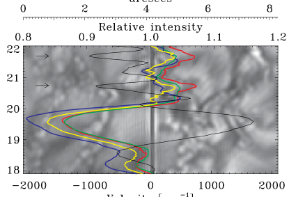
Figure 3.— One of the snapshots shows the spectrograph’s slit crossing a flower/ribbon (20$\farcs$8–22$\farcs$7) and a granule (18$\farcs$5–20$\farcs$0). The velocities are shown as measured in the Fe I 5379.6 Å line at intensity level 0.85 (red) and 0.65 (green), in the C I line (blue) and in the Fe I 5386.3 Å line at intensity level 0.85 (yellow). Positive velocities mean downflow. The black line shows the relative continuum intensity in the spectrogram. The two IGMs are marked with arrows.

A statistical analysis of the minimum LOS velocity within flowers and ribbons (Ribbon centers or RC) gives us velocities around zero m s^-1 in the Fe I 5379 Å line, while the the C I line shows an up flow of about 300 m s^-1. The Fe I 5386 Å shows a small upflow inside RCs with a mean of about 200 m s^-1. The standard deviations are of the order 100–200 m s^-1 in the Fe I lines, while the C I line has a standard deviation of about 350 m s^-1. These results are hampered with relatively high uncertainties of a few hundred m s^-1. We therefore want to investigate the effects of smearing along the line of sight and spatially on these velocity measurements.

We have also measured velocities inside bright points but since the spatial extent of each bright point is small they are difficult to identify. Nevertheless we visually classify 15 bright points and measure the velocities at intensity maximum. We measure a mean downflow of a few hundred m s^-1, but the velocities inside bright points vary a lot, and we also measure upflows inside some of the bright points. The standard deviation is quite high, about 0.5 km s^-1. Due to the small spatial extent of each bright point, the measured velocities are strongly affected by the surrounding intergranular velocity.

The effect of a non-zero g-factor is increased broadening in magnetic areas. For a non-symmetric profile this broadening may also introduce a change in the determined bisector. We have quantified this effect by applying a Zeeman splitting corresponding to a magnetic field strength of 1000 Gauss to the observed profiles and redetermined the bisector. The change in measured velocity is less than 40 m s^-1.

5. Simulations

Since the intensity level can be considered as a height parameter it is in principle possible to obtain the velocity as a function of absolute physical height. In order to explore this possibility we need a good model with which we can calibrate the velocities with height. One very suitable model is the magneto-convective simulation used by Carlsson et al. (2004). In this realistic simulation we can see bright points as well as more elongated magnetic structures. To tailor this simulation to our observational setup we use 12 atmospheric snapshots, including the same snapshot as the one used by Carlsson et al. (2004), with one minute time difference between the snapshots. We solve the equations of radiative transfer in LTE for these 3D atmospheres, using the MULTI code (Carlsson, 1986), for 1364 frequency points spanning from 5377.6 Å to 5389.4 Å. A line list of 249 lines is used. The line data was retrieved from the Vienna Atomic Line Database (VALD) (Kupka et al., 1999; Piskunov et al., 1995; Ryabchikova et al., 1999), with a few exceptions; the C I oscillator strength is taken from Hibbert et al. (1993) and an Fe line at 5382.5 Å was removed due to obvious errors in its central wavelength and oscillator strength.

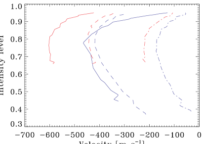
Figure 4.— From the FTS solar atlas, the total magnetic simulation and the total non-magnetic simulation we derive the bisectors in the two Fe I lines. The mean bisectors in the Fe I 5379 line (blue) and the Fe I 5386 Å line (red) in the FTS atlas (solid), the non-magnetic simulation (dashed), and in the magnetic simulation (dashed-dotted) are shown. The shift in the Fe I 5386 Å line indicate that there might be an error in the laboratory wavelength of about 100 m s^-1. Furthermore the laboratory wavelength of the Fe I 5379 Å seems to be well determined. Also notice the reduced blueshifts in the magnetic simulation of approximately 200 m s^-1, which are in good agreement with observational results.

A temporally and spatially averaged mean spectrum over 12 minutes and $8\farcs{27}\times 8\farcs{27}$, totally over 750000 spectra, is constructed. Since the simulation is covering an active region we expect the mean spectrum to have less blueshift, have shallower lines and to have more vertical lower bisectors (intensity level less than 0.7) than similar mean spectra obtained in non-magnetic regions (Brandt & Solanki, 1990, and references therein). For reference we therefore solve the equations of radiative transfer in LTE in three non-magnetic snapshots with 1 minute cadence, totally over 190000 spectra. Even though the temporal sampling is quite low we believe that the difference from a bigger temporal sample will be within 1 mÅ or approximately 50 m s^-1. In the non-magnetic simulation we have deeper strong Fe lines than the atlas, this is due to NLTE effects (Shchukina & Trujillo Bueno, 2001). The Fe lines in the mean magnetic spectrum do not show any reduced line depth. This might be because the magnetic field in the simulation is too weak but also because of NLTE effects. The convective blueshifts are in general well reproduced in the non-magnetic simulation (Asplund et al., 2000). One difference is that the upper part of the bisector shows larger blueshift than the atlas, see Fig.4. We therefore use the blueshift in the magnetic simulation as reference wavelength for the C I line since this simulations seems to give a more realistic convective blueshift in this line, see § 4. The magnetic simulation shows a blueshift that is about 200 m s^-1 smaller than the non-magnetic simulation, very similar to what was found observationally by (Brandt & Solanki, 1990). Furthermore the lower part of the bisector in the magnetic simulation is more vertical than in the non-magnetic simulation, also similar to observations. These are indications that the simulations are reproducing the velocities in a realistic manner.

When we measure the velocity in a spectral line at a given intensity level there are two smearing effects that will influence the measurement. The first effect is an intrinsic property of the line formation mechanism, namely the finite width of the response function. The response to a given velocity at a given height in a spectral line at a given intensity level is given by the response function to velocity at this intensity level (Magain, 1986). We calculate the response functions numerically using a step function in the velocity, very similar to the way Fossum & Carlsson (2005) calculate their response functions to perturbations in temperature. Typical response functions will have a pronounced peak but with a significant width of a few hundred kilometers, see Fig.5–6 for some examples. In Table 4 we give average response heights (given as the first order moment) in six different solar features (see Fig.5 and Fig.7 for definition). These response heights are calculated in the line core (LC) and in the close to continuum line wing (CLW) for the two Fe I lines while the moment of the total line (TL) was used for the C I line.

First order moment of the response functions.
	Fe I 5379 Å		Fe I 5386 Å		C I
Feature	LC	CLW	LC	CLW	TL
	[Km]	[Km]	[Km]	[Km]	[Km]
RC	232	32	46	-28	2
IGM	129	29	78	34	50
BP	-36	-112	-44	-116	-134
G	305	156	205	141	135
LMC	79	-123	-76	-170	-183
IG	248	127	211	143	141

Table 4

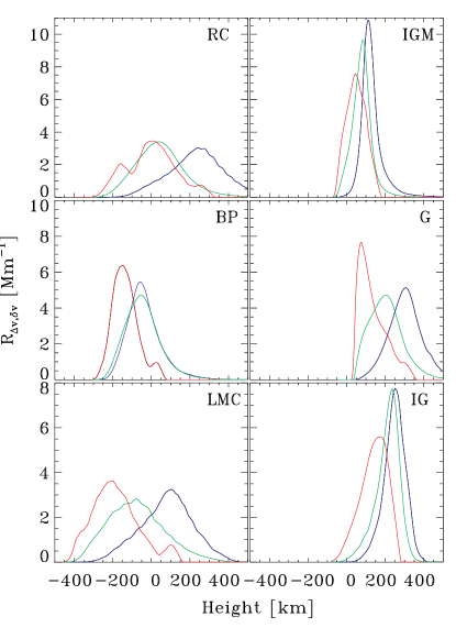
Figure 5.— Some typical response functions to velocity. The response function of the total C I line Doppler shift(red), and of the line core Doppler shift for the Fe I 5379.6 Å line (blue) and Fe I  5386.3 Å line (green) are shown. The different panels show from upper left to lower right: Ribbon center (RC), Intergranular lane close to Magnetic element (IGM), Bright point (BP), Granule (G), Large Magnetic Concentration (LMC), Inter granular lane (IG). The different points are defined in Fig.7, the BP, G, LMC, and IG are the same points as those used by Carlsson et al. (2004).

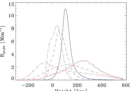
Figure 6.— Height variation of the response functions in the Fe I 5379 Å line in the Ribbon center (RC) (red) and the Intergranular lane close to Magnetic element (IGM) (blue). The intensity levels are 0.4 (solid), 0.6 (dashed) and 0.8 (dot-dashed). These intensity levels roughly correspond to the line core (LC), the mean line wing at the mean intensity level between the LC and local continuum, and the line wing close to continuum (CLW) respectively.

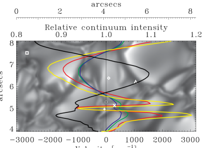
Figure 7.— Granule and a ribbon as they appear in the simulations are shown in this simulated slit-jaw image. The plasma velocity at the height where we have an atmospheric temperature equal to the radiation temperature at an intensity level (IL) of 0.65 is given in yellow, the non-convolved measured velocity at IL=0.65 in the Fe I 5379 Å line is given in red, while the green and blue lines show the convolved measured velocity at IL=0.85 and IL=0.65 respectively in the Fe I 5379 Å. The relative slit continuum intensity is shown in black. In Fig.5 we show response functions for different solar structures, these structures are defined in this figure: $+$ shows RC, $\circ$ shows IGM, $\times$ shows BP, $\Diamond$ shows G, $\Box$ shows LMC, and $\triangle$ shows IG.

The width of the response functions means that we do not measure the real plasma velocity but rather a height smeared velocity. The difference between the response function weighted velocity and the velocity at monochromatic optical depth unity can be several hundred m s^-1, see Fig.7. It is thus important to be aware of this effect when one talks about Doppler shifts measured in spectral lines. The response function to velocity in the IGM is quite narrow at all intensity levels, while the response function in the RC is much wider, see Fig.6. The effect of the response function smearing is, however, much higher in the IGM since the actual atmospheric velocity is changing much more quickly with height in IGMs than in RCs. This explains why we measure almost the exact plasma velocity in the RC in Fig.7 while we measure lower velocities in the IGM.

The second effect is the spatial smearing that originates from atmospheric seeing, the diffraction pattern of the telescope and scattering in the atmosphere, the telescope and the spectrograph. Even if we could determine the total point-spread function (PSF) of the atmosphere-telescope-spectrograph system, we can’t correct for these effects in the measured spectra since we have spectral information only along the one dimension of the slit. Another approach is to model the PSF and convolve the simulations with such a model to quantify the effects of the PSF on the measurements. The PSF of a partially AO corrected image for short exposures is usually assumed to consist of a diffraction core and a seeing halo from uncorrected or partially corrected modes. We assume that we can use this model for our spectra even though 80 ms is longer than what is normally accepted as short exposure. Furthermore we assume that the seeing halo has the form of a Lorentzian (Nordlund, 1984). Our model PSF thus has two free parameters: the width of the Lorenzian and the fraction of the Lorentzian component compared with the Airy core. A more detailed model of the PSF chould not be obtained since we lack the statistics necessary for the determination of more than two parameters. The observable is the continuum intensity distribution as measured in the spectra, excluding the pore. We assume that the intensity distribution in the simulations is realistic and compare the normalized distribution function of the intensities in the smeared simulation with the observed distribution function to determine the parameters. We find a good fit with a Lorentzian with FWHM of 0$\farcs$7 having a fraction of 0.1 at the center of the PSF, see Fig.8. The Strehl ratio of this PSF is 0.15 which is low compared with what one would expect from the AO system of the SST. One should remember here that we have no separate component to describe the scattering of the Earth’s atmosphere, which is known to be very wide, and the Strehl ratio obtained includes this effect. It is also important to point out that a range of parameters give acceptable fits to the observed intensity distribution function — wider Lorentzians with smaller fraction gives almost the same effect on the normalized distribution functions as a narrower Lorentzian with larger fraction. To check the sensitivity of the results to the PSF, we have performed tests both with a wider central core than the Airy disk and with different combinations of the width and fraction of the Lorentzian. As long as the normalized distribution function is close to the observed one we do not see significant changes in the resulting velocities (in comparison with the standard deviations shown in Fig.9). At the same time, the velocities determined from the convolved simulations are very different from the velocities in the unconvolved simulation. This may seem contradictory but is due to the fact that intensities and velocities are correlated — high intensity granules have large upflows, low intensity intergranular lanes downflow. When the PSF gives the observed intensity distribution function this also implies a similar effect on the velocity distribution function. Before comparing with observations, the spectral domain is convolved with the theoretical resolution of the TRIPPEL spectrograph.

Figure 8.— To mimic the atmospheric seeing we convolve the simulations with a linear combination of a Lorentzian and the Airy disk. The resulting NDFs for the observed spectra (solid), the unconvolved simulation (dashed), and the convolved simulation (dot-dashed) are shown.

Central wavelengths
and convective blueshifts in the simulations
Atomic	Simulation	Reference	Velocity
species	[Å]	[Å]	[m s-1]
Fe I	5379.5728	5379.5740	-69
C I	5380.3143	5380.3262	-664
Fe I	5386.3301	5386.3341	-223

Table 5

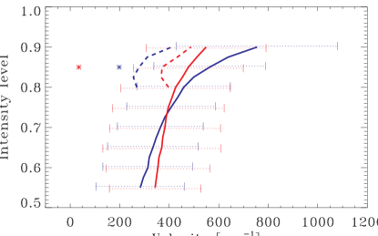
Figure 9.— Measured velocities in the IGMs in the observations (blue) and in the simulations (red) measured at different intensity levels for the Fe I 5379 Å line (solid), the Fe I 5386 Å line (dashed) and the C I line (asterisks). The standard deviations for the Fe I 5379 Å line are shown with error bars in the respective colors.

We use the laboratory wavelengths as reference wavelengths for the Fe I lines, while we use the same wavelength as in the observations for the C I line. Furthermore we calculate the central wavelength in the simulated atlas and the corresponding blue shift. The results are shown in Table 5 (with negative velocity meaning blueshift).

Now we can measure the velocities in the IGMs in the simulations. This is done in a similar manner as we measured the velocities in the IGMs in the observations, the results are plotted together with the observed results in Fig.9. The absolute velocities in the simulations and the observations differ with 200 m s^-1 or less, which is amazingly close when one consider the uncertainty in the observations of about 100–200 m s^-1 and that the standard deviation is about 200 m s^-1. Note that we believe that the Fe I 5386 Å line has an error of about 100 m s^-1 in the laboratory wavelength. This will increase the measured velocities with the same amount. Furthermore we see an increase in measured velocity with intensity level for both the observations and the simulations. This increase is somewhat lower in the simulation than in the observations. Note that the C I line gives substantially lower downflow values than the iron lines at comparable intensity level. This is true both in the observations and in the simulations. In the latter, the determined velocity is completely independent on the reference wavelength used so an error in the reference wavelength is not the explanation for the low velocities in the observations. The explanation is rather the differences in the response functions and the spatial smearing due to the seeing. The difference between the response functions in the IGM is minimal, but the difference between the response functions in granules is substantial. In the granule the C I line is formed deeper in the atmosphere, and hence this line will show a larger upflow. When the spatial smearing is applied this difference will lead to a smaller downflow in IGMs in the C I line, as observed. It is clear that the simulations and the observations are not in disagreement, even though there is room for improvements.

We also measure the lowest velocities within the magnetic elements in the simulation. The velocities measured range from about 200 m s^-1 upflow to about 200 m s^-1 down flow. The standard deviation is 250–300 m s ^-1. Due to the lack of good sampling of bright points in the simulations we do not include any statistics on bright points in the simulations.

6. Conclusions

We have presented spectrograms of small scale magnetic structures with excellent spatial resolution. These spectrograms have been used to measure the LOS velocities in several different magnetic structures. At the edges of the ribbons and flowers we measure downflow with an increasing magnitude with depth in the atmosphere. The magnitude of the downflow is about 200–700 m s^-1 with increasing velocity deeper down in the atmosphere. Inside the ribbons and flowers we measure a small upflow. The upflows are usually in the range 100–300 m s^-1. Our investigation of the velocities inside bright points shows both up and downflow, nevertheless with a mean downflow of a few hundred m s^-1. In most cases the velocity is closely related to the intergranular velocity, which indicate a strong presence of scattered light in the measured velocity.

Furthermore we have investigated the processes that are involved in the smearing of the measured velocities. The results from this work can be summarized as follows:

1. We have calculated response functions and response heights for several different solar features. The width of the response functions is usually a few hundred km.

2. We have convolved the simulations with a simple model of the point spread function of the observations. Due to the strong horizontal gradients in the velocity field in and close to small scale magnetic features, this spatial smearing has a strong effect on the measurements: the measured velocities in the intergranular lanes close to magnetic elements are decreased with about 1 km s^-1.

3. Since the simulations are reproducing the observations reasonably well we believe that the plasma velocities in the simulations are close to the real solar plasma velocities. In particular the velocities in and close to larger magnetic structures such as ribbons are well reproduced. The velocity in the simulation in intergranular lanes close to magnetic structures increases from about 1.5 km s^-1 at 150 km height to 3.3 km s^-1 at 0 km.

The velocity inside bigger magnetic structures such as ribbons in the simulations is about 1–2 km s^-1 upflow, with the velocity changing only a few hundred m s^-1 throughout the formation height between about $-$100 km and 250 km.

References

- Allende Prieto & Garcia Lopez (1998) Allende Prieto, C., & Garcia Lopez, R. J. 1998, A&AS, 129, 41
- Asplund et al. (2000) Asplund, M., Nordlund, Å., Trampedach, R., Allende Prieto, C., & Stein, R. F. 2000, A&A, 359, 729
- Berger et al. (2004) Berger, T. E., Rouppe van der Voort, L. H. M., Löfdahl, M. G., Carlsson, M., Fossum, A., Hansteen, V. H., Marthinussen, E., Title, A., & Scharmer, G. 2004, A&A, 428, 613
- Brandt & Solanki (1990) Brandt, P. N., & Solanki, S. K. 1990, A&A, 231, 221
- Brault & Neckel (1987) Brault, J., & Neckel, H. 1987, Hamburg Observatory anonymous ftp: ftp.hs.uni-hamburg.de
- Carlsson (1986) Carlsson, M. 1986, A Computer Program for Solving Multi-Level Non-LTE Radiative Transfer Problems in Moving or Static Atmospheres (Uppsala Astronomical Observatory: Report No. 33)
- Carlsson et al. (2004) Carlsson, M., Stein, R. F., Nordlund, Å., & Scharmer, G. B. 2004, ApJ, 610, L137
- Dravins et al. (1981) Dravins, D., Lindegren, L., & Nordlund, A. 1981, A&A, 96, 345
- Dunn & Zirker (1973) Dunn, R. B., & Zirker, J. B. 1973, Sol. Phys., 33, 281
- Fossum & Carlsson (2005) Fossum, A., & Carlsson, M. 2005, ApJ, 625, 556
- Hibbert et al. (1993) Hibbert, A., Biemont, E., Godefroid, M., & Vaeck, N. 1993, A&AS, 99, 179
- Johansson (1966) Johansson, L. 1966, Ark.Fys., 31, 201
- Keller et al. (2004) Keller, C. U., Schüssler, M., Vögler, A., & Zakharov, V. 2004, ApJ, 607, L59
- Kiselman et al. (2001) Kiselman, D., Rutten, R. J., & Plez, B. 2001, in IAU Symposium, p.287
- Kupka et al. (1999) Kupka, F., Piskunov, N., Ryabchikova, T. A., Stempels, H. C., & Weiss, W. W. 1999, A&AS, 138, 119
- Langhans et al. (2004) Langhans, K., Schmidt, W., & Rimmele, T. 2004, A&A, 423, 1147
- Langhans et al. (2002) Langhans, K., Schmidt, W., & Tritschler, A. 2002, A&A, 394, 1069
- Livingston et al. (1977) Livingston, W., Milkey, R., & Slaughter, C. 1977, ApJ, 211, 281
- Magain (1986) Magain, P. 1986, A&A, 163, 135
- Nave et al. (1994) Nave, G., Johansson, S., Learner, R. C. M., Thorne, A. P., & Brault, J. W. 1994, ApJS, 94, 221
- Neckel & Labs (1984) Neckel, H., & Labs, D. 1984, Sol. Phys., 90, 205
- Nordlund (1984) Nordlund, A. 1984, in Small-Scale Dynamical Processes in Quiet Stellar Atmospheres, ed. S. L. Keil (Sunspot: Sacramento Peak Obs.), 174
- Piskunov et al. (1995) Piskunov, N. E., Kupka, F., Ryabchikova, T. A., Weiss, W. W., & Jeffery, C. S. 1995, A&AS, 112, 525
- Rimmele (2000) Rimmele, T. R. 2000, in Proc. SPIE Vol. 4007, p. 218-231, Adaptive Optical Systems Technology, Peter L. Wizinowich; Ed., ed. P. L. Wizinowich, 218–231
- Rimmele (2004) Rimmele, T. R. 2004, ApJ, 604, 906
- Rouppe van der Voort et al. (2005) Rouppe van der Voort, L. H. M., Hansteen, V. H., Carlsson, M., Fossum, A., Marthinussen, E., van Noort, M. J., & Berger, T. E. 2005, A&A, 435, 327
- Rutten et al. (2001) Rutten, R. J., Kiselman, D., Rouppe van der Voort, L., & Plez, B. 2001, in ASP Conf. Ser. 236: Advanced Solar Polarimetry – Theory, Observation, and Instrumentation, ed. M. Sigwarth, p.445
- Ryabchikova et al. (1999) Ryabchikova, T., Piskunov, N., Stempels, H., Kupka, F., & Weiss, W. 1999, Physica Scripta, T83, 162
- Sánchez Almeida et al. (2001) Sánchez Almeida, J., Asensio Ramos, A., Trujillo Bueno, J., & Cernicharo, J. 2001, ApJ, 555, 978
- Scharmer et al. (2003a) Scharmer, G. B., Bjelksjö, K., Korhonen, T. K., Lindberg, B., & Petterson, B. 2003a, in Innovative Telescopes and Instrumentation for Solar Astrophysics. Edited by Stephen L. Keil, Sergey V. Avakyan . Proceedings of the SPIE, Volume 4853, pp. 341-350
- Scharmer et al. (2003b) Scharmer, G. B., Dettori, P. M., Löfdahl, M. G., & Shand, M. 2003b, in Innovative Telescopes and Instrumentation for Solar Astrophysics. Edited by Stephen L. Keil, Sergey V. Avakyan . Proceedings of the SPIE, Volume 4853, pp. 370-380
- Shchukina & Trujillo Bueno (2001) Shchukina, N., & Trujillo Bueno, J. 2001, ApJ, 550, 970
- Sobotka et al. (1994) Sobotka, M., Bonet, J. A., & Vazquez, M. 1994, ApJ, 426, 404
- Steiner et al. (2001) Steiner, O., Hauschildt, P. H., & Bruls, J. 2001, A&A, 372, L13
- Title & Berger (1996) Title, A. M., & Berger, T. E. 1996, ApJ, 463, 797
- van Noort et al. (2005) van Noort, M., Rouppe van der Voort, L., & Löfdahl, M. G. 2005, Sol. Phys., 228, 191
- von der Luehe (1993) von der Luehe, O. 1993, A&A, 268, 374