Evidence for a large fraction of Compton-thick quasars at high redshift

Abstract

Using mid-infrared and radio selection criteria, we pre-select a sample of candidate high-redshift type-2 quasars in the Subaru XMM-Newton Deep Field (SXDF). To filter out starburst contaminants, we use a bayesian method to fit the spectral energy distributions (SEDs) between 24-$\mu$m and B-band, obtain photometric redshifts, and identify the best candidates for high-$z$ type-2 quasars. This leaves us with 12 $z_{\rm phot}\geq 1.7$ type-2 quasar candidates in an area $\sim 0.8$ deg², of which only two have secure X-ray detections. The two detected sources have estimated column densities $N_{\rm H}\sim$2 & $3\times 10^{27}$ m^-2, i.e. heavily obscured but Compton-thin quasars. Given the large bolometric luminosities and redshifts of the undetected objects, the lack of X-ray detections suggests extreme absorbing columns $N_{\rm H}\mathrel{\hbox{\hbox to0.0pt{\hbox{\lower 2.0pt\hbox{$\sim$}}\hss}\raise 2.0pt\hbox{$>$}}}10^{28}$ m^-2 are typical. We have found evidence for a population of “Compton-thick” high-redshift type-2 quasars, at least comparable to, and probably larger than the type-1 quasar population, although spectroscopic confirmation of their AGN nature is important.

1 Introduction

High-redshift quasars with column densities $N_{\rm H}\mathrel{\hbox{\hbox to0.0pt{\hbox{\lower 2.0pt\hbox{$\sim$}}\hss}\raise 2.0pt\hbox{$>$}}}10^{28}$ m^-2 are so heavily absorbed that they are barely detectable in even the most sensitive hard X-ray surveys (see, e.g., Brandt & Hasinger, 2005), and are known as “Compton-thick”. While in the local Universe, 40% of active galactic nuclei (AGN) are found to be Compton-thick (Risaliti et al., 1999), the fraction of high-redshift quasars with such absorbing columns is currently unknown.

An alternative to (hard) X-ray selection is in the mid-infrared, where the obscuration due to dust becomes small. AGN are powerful mid-infrared emitters due to dust surrounding the accretion disk (the torus) reprocessing the UV and X-ray photons from the central engine. AGN invisible in X-rays were indeed found by Donley et al. (2005), who used a mid-infrared and radio excess criterion to to select a sample of AGN. The majority of these AGN are at $z\mathrel{\hbox{\hbox to0.0pt{\hbox{\lower 2.0pt\hbox{$\sim$}}\hss}\raise 2.0pt\hbox{$<$}}}1$ and are better described as Seyfert-2s by virtue of their low luminosities. The authors found that while the sources detected in the X-ray were unlikely to be Compton-thick, the AGN not detected in the X-ray ($\sim$20% of their sample) could be Compton-thick ($N_{\rm H}$$\mathrel{\hbox{\hbox to0.0pt{\hbox{\lower 2.0pt\hbox{$\sim$}}\hss}\raise 2.0pt\hbox{$>$}}}10^{28}$ m^-2). The obscured and gravitationally-lensed quasar IRAS FSC 10214+4724, at $z\sim 2.3$ also appears to be Compton-thick (Alexander et al., 2005).

Polletta et al. (2006) use two different selection criteria, X-ray and infrared, to look for Compton-thick AGN in an area of 0.6 deg². Their X-ray selection, with a flux limit $\sim$10^-17 W m^-2 in the 2.5-8 keV band, finds 5 Compton-thick AGN. Of these 2 are spectroscopically confirmed high-redshift quasars. Of the infrared-selected sources, the strict SED criteria imposed on the sources guarantee AGN, but are likely to exclude heavily obscured ($A_{\rm V}\mathrel{\hbox{\hbox to0.0pt{\hbox{\lower 2.0pt\hbox{$\sim$}}\hss}\raise 2.0pt\hbox{$>$}}}20$) high-redshift ($z\geq 1$) sources which do not show power-law mid-infrared spectral energy distributions (SEDs), but have significant contributions from stellar light at 3.6 and 4.5 $\mu$m. It is not suprising, therefore, that they find a smaller Compton-thick fraction ($\sim$10%) than expected in their infrared-selected sample, as it is probably biased against heavily obscured AGN. At high luminosities and redshift, Alonso-Herrero et al. (2006, AH06) find $\sim$50% of their sources are undetected in X-rays (although not necessarily Compton-thick). This sample is based on a power-law criterion, and could plausibly also be missing the most heavily obscured sources.

Martínez-Sansigre et al. (2005), hereafter MS05, found a population of high-redshift type-2 quasars at least as numerous as the unobscured (type-1) population and which possibly outnumber the type-1s by $\sim$2-3:1. The most recent X-ray studies agree with a large obscured fraction but disagree on the relative numbers of Compton-thick sources: Dwelly & Page (2006, DP06) find a $\sim$3:1 ratio amongst Compton-thin type-2 and type-1 quasars, while Gilli, Comastri & Hasinger (2006) infer a $\sim$1:1 ratio of Compton-thin type-2 to type-1 quasars, although the total type-2 to type-1 ratio can increase to $\sim$2:1 when Compton-thick sources are included.

In this letter, we present the X-ray properties of a sample of obscured (type-2) high-redshift quasars, selected from mid-infrared and radio data in the Subaru XMM-Newton Deep Field (SXDF).

2 Sample selection and dataset

We proceed to select a similar sample to that of MS05, in the SXDF, where deep X-ray data are available. In this work we decrease the lower radio flux density criterion, to increase the number of candidates. This is important as here we have a smaller area ($\sim$0.8 deg² as opposed to 3.8 deg² in the MS05 sample). The selection criteria used here are $S_{24~{}\mu\rm m}>300~{}\mu$Jy, $S_{3.6~{}\mu\rm m}\leq 45~{}\mu$Jy, and 100 $\mu$Jy $\leq S_{1.4\rm GHz}\leq$ 2 mJy, which yields 38 candidates. For a detailed discussion of these criteria see Martínez-Sansigre et al. (2006a, hereafter MS06).

As a brief summary, the two mid-infrared criteria are able to target $z\sim 2$ type-2 quasars with $A_{\rm V}\mathrel{\hbox{\hbox to0.0pt{\hbox{\lower 2.0pt\hbox{$\sim$}}\hss}\raise 2.0pt\hbox{$>$}}}5$, but will also allow $z\mathrel{\hbox{\hbox to0.0pt{\hbox{\lower 2.0pt\hbox{$\sim$}}\hss}\raise 2.0pt\hbox{$<$}}}1$ ultra-luminous infrared galaxies (ULIRGs) in the sample. These ULIRGs will have radio luminosities following the FIR-radio correlation (Condon, 1992), and so by choosing a high-enough radio flux, one can cut out all but the most extreme starburst contaminants. The MS05 criteria were carefully chosen to avoid starburst galaxies, and lowering the radio criterion has the disadvantage that less extreme starbursts are allowed in the sample.

The mid-infrared data were obtained by using the SWIRE DR2 (Surace et al., 2005), which covers the SXDF, and has a flux density limit of $\sim$250 $\mu$Jy at 24 $\mu$m (5$\sigma$), and 10 $\mu$Jy for both 3.6 and 4.5 $\mu$m (10$\sigma$ and 5$\sigma$ respectively). The 1.4 GHz catalogue used is described in Simpson et al. (2006) and comes from a B-array ($\sim$5$\times$4 arcsec² beam) VLA survey with a peak flux density limit of 100 $\mu$Jy ($\sim$5-8 $\sigma$).

The spectroscopic completeness of the SXDF are poor at this stage, so we decided to undertake this preliminary study using photometric redshifts (see Section 3). The optical data were obtained from the Subaru B,V,R,i’ and z’ imaging (Furusawa et al., in prep.). The near-infrared data (J and K) were taken from the UKIDSS ultra-deep survey (UDS) DR1 (Warren et al., 2007). The X-ray data were obtained with the XMM-Newton observatory, which covered the SXDF field in 7 pointings, with exposures of 50 ks each, except for the central pointing, which was observed for 100 ks (Ueda et al., in prep.).

Name	RA	Dec	$z_{\rm phot}$	log10[$L_{\rm bol}$	$A_{\rm V}$	log10[$L_{\rm gal}$	log10[$L_{\rm blue}$	ln[OR(q/u)]	log10[p(d$|$q)/	$S_{2-12\rm keV}$
	(J2000)			/W]		/$L^{*}_{\rm k}$]	/$L^{*}_{\rm k}$]		($S_{17}$)12/]	/ $S_{17}$
ID052	02 16 17.92	-05 07 18.56	1.90$\pm 0.05$	41.21	119	0.85	0.55	13.0	-10.0	$<$0.7
ID123	02 19 28.76	-05 09 08.81	1.75$\pm 0.05$	40.2	72	0.65	0.20	5.2	-9.7	$<$2.92
ID135	02 19 01.89	-05 11 14.22	4.15${}_{-0.09}^{+0.05}$	40.2	2.23	1.20	0.15	26.0	-9.4	$<$0.3
ID142	02 17 23.82	-04 35 13.72	4.05$\pm 0.05$	40.4	6.7	1.25	0.45	10.0	-8.9	$<$0.4
ID147	02 19 10.31	-05 16 03.00	1.80$\pm 0.05$	40.1	35.9	0.75	-0.05	28.6	-13.4	$<$0.3
ID200	02 18 15.71	-05 05 10.34	1.75${}_{-0.07}^{+0.05}$	40.1	72	0.75	0.50	8.4	-9.1	$<$0.4
ID249	02 19 13.74	-04 56 04.27	1.75$\pm 0.05$	40.0	35.9	0.50	0.00	25.2	-9.2	$<$0.6
ID342	02 17 05.35	-05 09 24.61	3.85$\pm 0.05$	40.0	9.0	1.20	0.30	4.6	-15.25	$<$6.82
ID345	02 16 29.56	-05 03 10.65	2.00${}_{-0.07}^{+0.08}$	39.8	35.94	1.00	0.10	10.4	-11.1	$<$0.6
ID347	02 18 09.64	-05 18 42.42	1.75$\pm 0.05$	40.2	72	0.55	-0.30	5.8	-8.0	1.7$\pm$0.95
ID386	02 17 25.11	-05 16 17.27	1.90${}_{-0.12}^{+0.05}$	39.4	17.9	0.50	-0.75	6.2	-11.5	$<$0.1
ID401	02 16 23.02	-05 08 06.76	1.90${}_{-0.12}^{+0.05}$	40.0	35.9	0.70	0.40	26.7	-8.9	3.4$\pm$1.35

Table 1: Best-fit parameters and X-ray fluxes for the high-redshift type-2 quasars. The names are from the radio catalogue of Simpson et al. (2006), and we define $S_{17}=10^{-17}$ W m^-2 for convenience. The errors in $z_{\rm phot}$ are estimated, given our model SEDs, from the full-width half-maximum values from the marginalised probability distribution functions (PDFs) for $z_{\rm phot}$. For most objects, the PDF has at least one secondary peak, always adjacent to the primary one, with peak value between 0.5 and 0.05 of the primary peak. The median value of log₁₀[$L_{\rm gal}$/$L^{*}_{\rm k}$], 0.75, corresponds to a 5.6$L^{*}_{\rm k}$ (where $L^{*}_{\rm k}$ is the break in the local K-band luminosity function) galaxy at $z\sim 2$, which asuming passive evolution and using the models of Bruzual & Charlot (2003), would become a present-day $\sim$$L^{*}_{\rm k}$ galaxy. The limits quoted for X-ray non-detections are the flux returned by the task EMLDETECT at the position of the source, plus the error quoted for this flux. This is approximately the same as a 2$\sigma$ limit. ¹This high value for $L_{\rm bol}$ is probably due to an overestimation of the $A_{\rm V}$. ²The reason for these high values for the fluxes is that the background noise is significantly higher in these two sources. ³This value of $A_{\rm V}$ suggests a reddened type-1 quasar rather than a genuine type-2. ⁴ID345 is a point source at K-band, which suggests the value of $A_{\rm V}$ is an overestimate. ⁵ID347 and ID401 have safe X-ray detections. The best-fitting SEDs for all 12 objects can be found at: http://www.mpia.de/homes/martinez/sxdftype2seds.pdf

3 Photometric redshifts and filtering out ULIRG contaminants

In order to disentangle type-2 quasars from ULIRGs and obtain photometric redshifts, the SEDs of the candidates were fitted using a model consisting of three components (warm dust, galaxy light and blue light). The normalisations of the components were allowed to vary together with the redshift, $z$, although for a given $A_{\rm V}$ and $z$, the normalisation of the warm dust component was fixed to fit the 24 $\mu$m data. Two different models were investigated, and the bayesian odds ratio (e.g. Sivia, 1996) was used to select between the models. These models differed only in their warm dust properties and consisted of a quasar (with dust) and a ULIRG. The redshift was given a flat prior between $0\leq z\leq 7$. No real quasars have been detected at $z\mathrel{\hbox{\hbox to0.0pt{\hbox{\lower 2.0pt\hbox{$\sim$}}\hss}\raise 2.0pt\hbox{$>$}}}7$, justifying this cutoff.

The stellar population was modelled by taking the SED of a $z=0$ elliptical galaxy from Coleman, Wu & Weedman (1980). SEDs showing smaller 4000-Å breaks were well fitted by the elliptical galaxy together with the blue component (see below). The elliptical was normalised to match the K-band luminosity of an $L^{*}$ galaxy in the local K-band luminosity function of Cole et al. (2001). The luminosity of the galaxy relative to the local $L^{*}_{\rm K}$ was then allowed to vary with a prior flat in log-space, between $-1.3\leq$log${}_{10}(L_{\rm gal}/L^{*}_{\rm K})$$\leq 1.3$. This choice brackets the reasonable range of host galaxies for a powerful quasar accounting for passive evolution: from a very faint $0.05L^{*}_{\rm K}$ to a very bright $20L^{*}_{\rm K}$ galaxy. The choice of a prior flat in log-space means that the host galaxy is believed, a priori, to be as likely to lie between $0.1L^{*}_{\rm K}$ and $L^{*}_{\rm K}$ as between $L^{*}_{\rm K}$ and $10L^{*}_{\rm K}$. This is more realistic than a prior flat in real space, which would imply a quasar is as likely to be hosted by an $L^{*}_{\rm K}$ galaxy as by a $10L^{*}_{\rm K}$ one.

The blue component, between 912 Å  and 5000 Å, has a physical motivation as well as serving a practical purpose. It can represent the scattered light from the obscured quasar, blue light from young stars or a UV-upturn brighter than that of the template elliptical galaxy used (and therefore a smaller 4000-Å break). The slope was therefore set to $S_{\nu}\propto\nu^{-0.5}$, which is representative of both type-1 quasars and starforming galaxies. The normalisation of the blue component is given as a ratio of the luminosity to that of an $L^{*}_{\rm K}$ galaxy at 5000 Å, and was allowed to vary independently of the galaxy, with a flat prior between $-2\leq$log${}_{10}(L_{\rm blue}/L^{*}_{\rm K,5000\AA})$$\leq 2$, spanning the range between a blue component fainter than an $L^{*}_{\rm K}$ elliptical galaxy’s UV-upturn, and as bright as the most powerful type-1 quasar. To avoid overfitting and losing the ability to discriminate between models, neither the stellar or the blue component are reddened by dust.

The ULIRG dust component was modelled using the models of Siebenmorgen & Kruegel (2007), hereafter SK07, only allowing variation of one parameter, $A_{\rm V}$. For a given $A_{\rm V}$ and $z$, the bolometric luminosity of the ULIRG, $L_{\rm bol}$ was chosen to make the SED go as close as possible to the 24-$\mu$m data point. The values of $L_{\rm bol}$ are only restricted by the range available in the SK07 library: $10.1\leq$ log${}_{10}(L_{\rm bol}/L_{\odot})$ $\leq 12.7$ for our choice of parameters. Of the other parameters, the nuclear radius was fixed to 1 kpc, the ratio of luminosity of OB stars with hot spots to $L_{\rm tot}$ was fixed to 0.6, and the hydrogen number density was fixed to $10^{10}$ m^-3. The models have a discreet set of values of the extinction ($A_{\rm V}=$ 2.2, 4.5, 6.7,9, 17.9, 35.9, 72 and 119), so the prior for the $A_{\rm V}$ consists of a set of $\delta$-functions (with equal probability) at these values.

The mid-infrared SED for quasars was modelled using the Elvis et al. (1994), hereafter E94, type-1 SED, and obscuring it with dust from the models of Pei (1992). For consistency with SK07, only Milky Way (MW)-type dust is used. This SED and dust model would allow us, in principle, to vary the values of $A_{\rm V}$ continuously, but to make the fitting procedure as fair as possible, we restricted the values of $A_{\rm V}$ to those present in the models of SK07 and assigned the same prior to them. This flat prior reflects our ignorance about the range in $A_{\rm V}$, particularly for quasars. For each object, the quasar bolometric luminosity $L_{\rm bol}$ was not allowed to vary freely, but was fixed for a given $A_{\rm V}$ and $z$ by the observed flux density at 24 $\mu$m. There is, however, no upper limit set on $L_{\rm bol}$.

For a given model, the likelihood of a given combination of parameters is given by the n-dimensional probability density function

$${\rm p(data|model~{}A,{\it z},{\it A_{\rm V}},{\it L_{\rm gal}},{\it L_{\rm blue}})}=$$

$${1\over(2\pi)^{n/2}\displaystyle\prod^{n}_{i}\sigma_{i}}e^{-\chi_{\rm A}^{2}/2},$$ (1)

where

$$\chi_{\rm A}^{2}=\displaystyle\sum^{n}_{i}{\rm(model~{}A_{\it i}-data_{\it i})}^{2}/\sigma_{\it i}^{2},$$ (2)

model A_i is the flux predicted by model A, given the parameters, over a given waveband, data_i is the observed flux at that band, $\sigma_{i}$ is the measurement error in that band and n is the number of bands. In the cases where $\sigma_{i}$ was smaller than 10% of the flux density of the object, it was set to 10%. To treat non-detections at a particular band, we followed the following method: when the observed galaxy flux density and the model fell below the flux density limit (5$\sigma_{band}$, where $\sigma_{band}$ is the rms noise in that band), the band made no contribution to $\chi^{2}$. When the model lay above the limit, the object was assigned a flux density $S_{i}$ and an error $\sigma_{i}$ both equal to half of the flux density limit (so $S_{i}=$$\sigma_{i}=2.5\sigma_{band}$). An undetected source would therefore only be 1$\sigma_{i}$ away from zero flux density, and from the limit. This prescription was appropriate for our sources, selected to be faint and therefore close to the limits in most of the bands, to avoid excessively penalising nondetections in one band.

To select between models, we follow Sivia (1996) in calculating the odds ratio (OR),

$${\rm OR(A/B)}={{\rm p(d|A)~{}p(A)}\over{\rm p(d|B)~{}p(B)}},$$ (3)

where, for brevity, we refer to model A as A, model B as B, and data as d. We assume that models A and B are equally likely a priori,  ${\rm p}(A)/{\rm p}(B)=1$, implying ignorance in the fraction of quasars c.f. starbursting galaxies. Thus the evidence for model y (where y $\in\{A,B\}$) is proportional to p(d$|$y), which is simply the likelihood (from eq 1) integrated over the parameter space spanned by the priors, i.e.:

$$\noindent{\rm p(d|y)}=$$

$$\int e^{-\chi_{\rm y}^{2}/2}{\rm p}(z){\rm p}(A_{\rm V}){\rm p}(L_{\rm gal}){\rm p}(L_{\rm blue})\it{\rm d}z{\rm d}A_{\rm V}{\rm d}L_{\rm gal}{\rm d}L_{\rm blue},$$ (4)

$\chi_{\rm y}^{2}$ is as defined in Equation 2, p($x$) is the normalised prior probability distribution of parameter $x$ and the integral is over the entire prior space. To make sure that our X-ray analysis did not include any ULIRGs, only objects with OR(quasar/ulirg)$\geq 100$ were considered as quasars. This is equivalent to stating we are at least 99% confident of the quasar model over the ULIRG model. Note this criterion is very similar to the so-called Jeffreys’ criterion (Jeffreys, 1961). In addition, to make sure the fits were acceptable, only sources with evidence p(data$|$quasar)$/(S_{17})^{12}\geq 10^{-17}$ were accepted, where $S_{17}=10^{-17}$ W m^-2 ($S_{17}$ is defined to avoid numbers of order $10^{-204}$ or smaller). Our range of evidences in Table 1, $1.3\times 10^{-9}\leq$p(data$|$quasar)$/(S_{17})^{12}$$\leq 5.5\times 10^{-16}$, corresponds approximately to values of reduced $\chi^{2}=1.9-6.1$. Finally, only sources with $z_{\rm phot}\geq 1.70$ were kept, since Ly $\alpha$ is visible in optical spectroscopy, so the redshifts can be checked observationally, as long as this line is not obscured by dust on large scales (see MS06). Preliminary spectroscopy of the sample suggests our values of $z_{\rm phot}$ are in good agreement with spectroscopic redshifts (A. Martínez-Sansigre et al. in prep.).

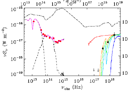
Figure 1: Best fit spectral energy distribution (SED) of ID401. The top x-axis and right y-axis show the rest-frame frequencies and luminosities (in units of $L_{\odot}$) assuming the best-fit $z_{\rm phot}=1.90$. The dashed black lines show (from left to right) the quasar (with extinction), galaxy and blue templates normalised by the values (from Table 1) alongside the best fit to the data (red dots), the solid purple line shows the combined best-fit templates. The black dots and limits are the X-ray data in the 0.3-0.5, 0.5-1, 1-2, 2-4.5 and 4.5-12 keV bands, from all three EPIC cameras. The coloured lines are the WF99 absorbed models, with values of log₁₀($N_{\rm H}$/ m^-2) = 25.00 (red), 27.25 (yellow), 27.50 (green), 27.75 (cyan) and 28.50 (dark blue), with normalisation so the unobscured curve (25.00) goes through the highest energy X-ray point. The X-ray datapoints are best described by the curve with 27.25 (yellow). For comparison, the E94 type-1 SED has been overplotted (dash-dotted line), with the same values of $L_{\rm bol}$ and $z_{\rm phot}$ as ID401 (from Table 1). The low value of the unobscured WF99 curve, compared to the E94 curve, shows this source has an intrinsically lower X-ray to mid-infrared ratio by a factor $\sim 3$, than the expectation of E94.

Of the 38 candidates in the sample, 12 (32%) follow our above criteria and are considered our best candidates for high-redshift type-2 quasars. Their best-fit parameters are quoted in Table 1, and we proceed to analyse the X-ray properties of these sources. Visual inspection of the optical images showed several cases where the blue light was unresolved. This fits in well with scattered light from the quasar reaching us and justifies our choice of a “blue” component. Typically the best fitting normalisation for the blue component is $\sim$5% of the normalisation of the quasar component, which is a reasonable scattering fraction. The K-band images showed resolved sources in 11 cases, while ID345 is a point-source (suggesting a real $A_{\rm V}\mathrel{\hbox{\hbox to0.0pt{\hbox{\lower 2.0pt\hbox{$\sim$}}\hss}\raise 2.0pt\hbox{$<$}}}5$; a reddened type-1, see MS06). The SED and $A_{\rm V}$ of ID135 (see supplementary Figures) also suggest a reddened quasar, rather than a genuine type-2, although since it is not point-like in K-band, the host galaxy probably contributes significantly to the near-infrared flux.

4 X-ray properties of the type-2 quasars

The type-2 quasars were cross-matched with the X-ray catalogue of Ueda et al. (in prep.) with a flux limit of $\sim$3$\times 10^{-18}$ W m^-2 in the 2-12 keV band, but only 2 out of 12 (17%) were detected: ID347 and ID401. These objects have likelihoods (EP_DET_ML) of 81 and 80 respectively, and are therefore clear detections (see DP06 for an explanation of the likelihood).

To obtain meaningful limits for the undetected sources, these had their counts measured directly from the X-ray image, using the XMM-Newton Science Analysis Software (SAS). The positions of the sources not detected in the XMM-Newton observations were added manually to the EBOXDETECT source lists of each observation. We then ran the SAS task EMLDETECT keeping the positions of the sources fixed. EMLDETECT performs a maximum likelihood fit on the distribution of observed counts of the sources previously extracted by the task EBOXDETECT. The fit uses the five diferent energy bands (in keV: 0.2-0.5,0.5-1,1-2,2-4.5,4.5-12) and the three EPIC cameras (M1,M2,pn) simultaneously. This procedure allowed to fit the sources as multiple components with separate point-spread functions (PSFs), and sources with no evidence of any X-ray detection were still fitted.

This procedure allowed us to obtain fits to the counts for all sources in the 5 EPIC bands, and these were converted to fluxes in each band, assuming a photon index $\Gamma=1.7$ and an obscuring column of $N_{\rm H}=3\times 10^{24}$ m^-2 (the default SAS values). These are not the most likely values for obscured quasars, so we estimate the effects of using more representative values. Assuming instead $\Gamma=1.9$, $N_{\rm H}=3\times 10^{27}$ m^-2 at $z=2$ we estimate the change in fluxes to be only +9%, +3% and -2% in the 1-2, 2-4.5 and 4.5-12 keV bands, and therefore negligible compared to the large uncertainties in the count rates. All the 10 sources undetected in the Ueda et al. catalogue were found to have fitted values consistent with background noise, even in the hard band (see Table 1). We therefore find that 83% of our sources classified as high-redshift type-2 quasars are undetected in the X-ray image, even down to a flux limit of $\sim$3$\times 10^{-18}$ W m^-2 in the 2-12 keV band (the exact limit varies across the X-ray image).

5 Discussion

We have found that 10 out of 12 of our sources classified as type-2 quasars, are undetected in an X-ray image with an approximate flux limit $\sim$3$\times 10^{-18}$ W m^-2 (in the 2-12 keV band). For the two detections, we use the photometric redshifts and the Monte-Carlo models of Wilman & Fabian (1999, WF99) to estimate the absorbing columns. The estimates for ID347 and ID401 are log${}_{10}(N_{\rm H}/\rm m^{2})=$ 27.50 and 27.25 respectively (although ID347 requires a black body at 10⁷ K in addition to the WF99 spectrum, to fit an upturn in the soft X-rays). For both these objects, the intrinsic X-ray to mid-infrared ratio seems to be slightly lower than the E94 expectation by a factor $\sim$2-5.

For the undetected objects, it is not possible to estimate values of $N_{\rm H}$. However, as Figure 1 shows, the sensitivity of the XMM-Newton observations and the “negative K-correction” in X-rays mean that our X-ray data are sensitive to heavily obscured Compton-thin quasars, even if, like ID347 and ID401, at X-ray energies they are intrinsically weaker than our first expectation from the median SED of E94. Only when log${}_{10}(N_{\rm H}/\rm m^{2})\mathrel{\hbox{\hbox to0.0pt{\hbox{\lower 2.0pt\hbox{$\sim$}}\hss}\raise 2.0pt\hbox{$>$}}}$ 28.50, do sources with $L_{\rm bol}\sim 10^{40}$ W become too faint to be detected in the energy bands covering 2-12 keV (rest-frame $\sim$6-36 keV).

To get a handle of the possible values of $N_{\rm H}$, in Figure 2 we show fiducial tracks for a model quasar (see Figure caption for details). From this figure, the two detected objects in X-rays and two of the non-detections have values consistent with being heavily absorbed but Compton-thin, while the other 8 objects undetected in X-rays are likely to be Compton-thick. Spectroscopic confirmation of the AGN nature of our sources is now required.

Inspection of Figure 2 shows most of our objects populate a region of the $S_{2-12\rm keV}$ versus $S_{24~{}\mu\rm m}$ plane that is lacking in sources in previous work (e.g. AH06). The reason for this is that our selection criteria focus in on objects covering a fairly narrow range in redshift and bolometric luminosity over a fairly large sky area. Most previous studies (e.g. AH06) cover much larger ranges in z and luminosity with few objects like ours expected because of small sky area coverage and mid-IR selection techniques (such as mid-IR-power-law selection) that bias against the most obscured objects.

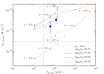
Figure 2: Hard X-ray flux ($S_{2-12\rm keV}$) versus 24-$\mu$m flux density ($S_{24~{}\mu\rm m}$) as a function of redshift for a model obscured quasar. This quasar has been chosen to have log${}_{10}(L_{\rm bol}/W)=40.1$ and $A_{\rm V}=35.9$, which are both the median values from Table 1. The quasar has the intrinsic SED of E94, with obscuring dust from the models of Pei (1992). We use the absorbed X-ray spectra of WF99, with four different absorbing columns, log${}_{10}(N_{\rm H}/{\rm m}^{-2})=$ 26.75, 27.50, 28.25 and 29.25. This corresponds to a range in gas-to-dust ratio of $N_{\rm H}/A_{\rm V}=1.9\times 10^{25}$ to $5\times 10^{27}$ m^-2 (the lower value being that of the Milky Way, the upper value being much larger but reasonable, see MS06 and Watanabe et al., 2004). The green and blue tracks are obscured but Compton-thin, the red track is mildly Compton-thick, while the yellow line is heavily Compton-thick. The black dots mark the values at particular redshifts. Changing the $A_{\rm V}$ to any other value of Table 1 would move the tracks horizontally only. The 12 type-2 quasars in our sample are overplotted in blue. The vertical dotted line is the 300 $\mu$Jy flux density limit imposed on our sample, the horizontal dotted line is the approximate flux limit of the X-ray image, $\sim 3\times 10^{-18}$ W m^-2. For our two X-ray detections, the independent estimates of log${}_{10}(N_{\rm H}/\rm m^{2})$ are $\sim 27.50$ so at first one expects them to follow the blue track. That these two objects lie significantly below the blue track is not a cause for serious worry as it assumes a fiducial unobscured QSO SED that is subject to population variance. To make the objects ID347 and ID401 consistent with the track would mean they have intrinisc X-ray to mid-infrared ratios $\sim 3\times$ lower than those of the assumed SED (E94, see also Figure 1). This ratio is consistent with the $\sim 1\sigma$ spread of the population used in E94. While the two non-detections with high limits are approximately consistent with ID347 and ID401 and the Compton-thin tracks, the remaining 8 sources are well below the expectations, suggesting they are Compton-thick.

Following MS05, we model the expected number of type-1 quasars following our 24-$\mu$m and radio flux density criteria, at $z\geq 1.70$, and in 0.8 deg². We predict 2$\pm 0.8$ type-1 quasars following these criteria, while we have 12 type-2 quasars of which 8 are likely Compton-thick. Assuming the error in the modelled number of type-1 quasars, and Poisson errors for the numbers of type-2 quasars, the type-2 to type-1 ratio (in the 68% confidence interval) is in the range 3.0-12.9 while the Compton-thick-type-2 to type-1 ratio is in the range 1.8-9.0.

Although we are clearly suffering from problems due to small-number-statistics, the implication of our study is that, at high redshift, Compton-thick quasars may be the dominant sub-population of quasars. Although such objects would be essentially absent from even moderately hard X-ray surveys (energy $\sim$2-10 keV), and their contribution to the hard X-ray background (energy $\geq$10 keV) is diluted by their large distances, they could clearly represent a vital part of the accretion history of black holes.

Our work to date (MS05, MS06) has included radio as well as mid-IR selection criteria. There is therefore a residual worry that the properties of the objects we have studied are influenced in some way by the presence of weak radio jets, and (Martínez-Sansigre et al.2006b) have shown that their radio properties are consistent with these objects having developed large-scale FRI-like jets. In principle, only mid-IR selection criteria are needed to find high-redshift quasars, although the difficulty lies in filtering out the starbursts from the quasars.

References

- Alexander et al. (2005) Alexander D. M., Chartas G., Bauer F. E., Brandt W. N., Simpson C., Vignali C., 2005, MNRAS, 357, L16
- Alonso-Herrero et al. (2006) Alonso-Herrero A., et al., 2006, ApJ, 640, 167
- Brandt & Hasinger (2005) Brandt W. N., Hasinger G., 2005, ARA&A, 43, 827
- Bruzual & Charlot (2003) Bruzual G., Charlot S., 2003, MNRAS, 344, 1000
- Cole et al. (2001) Cole S., et al., 2001, MNRAS, 326, 255
- Coleman et al. (1980) Coleman G. D., Wu C.-C., Weedman D. W., 1980, ApJS, 43, 393
- Condon (1992) Condon J. J., 1992, ARA&A, 30, 575
- Donley et al. (2005) Donley J. L., Rieke G. H., Rigby J. R., Pérez-González P. G., 2005, ApJ, 634, 169
- Dwelly & Page (2006, DP06) Dwelly T., Page M. J, 2006, MNRAS, 372, 1755
- Elvis et al. (1994) Elvis M., et al., 1994, ApJS, 95, 1
- (11) Gilli R., Comastri A., Hasinger G., 2007, A&A, 463, 79
- Jeffreys (1961) Jeffreys H., 1961, Theory of Probability. Oxford Univ. Press