Probing the internal solar magnetic field through g-modes

Abstract

The observation of g-mode candidates by the SoHO mission opens the possibility of probing the internal structure of the solar radiative zone (RZ) and the solar core more directly than possible via the use of the p-mode helioseismology data. We study the effect of rotation and RZ magnetic fields on g-mode frequencies. Using a self-consistent static MHD magnetic field model we show that a 1% g-mode frequency shift with respect to the Solar Seismic Model (SSeM) prediction, currently hinted in the GOLF data, can be obtained for magnetic fields as low as 300 kG, for current measured modes of radial order $n=-20$. On the other hand, we also argue that a similar shift for the case of the low order g-mode candidate ($l=2$, $n=-3$) frequencies can not result from rotation effects nor from central magnetic fields, unless these exceed 8 MG.

1 Introduction

The observation of g-mode candidates by the Global Oscillation at Low Frequencies (GOLF) instrument aboard the ESA/NASA Solar and Heliospheric Observatory (SoHO) mission (Turck-Chièze et al., 2004) opens new prospects for solar physics. Indeed, it brings the possibility of probing the internal structure of the solar radiative zone (RZ) and the solar core more efficiently and more directly than possible via the use of the p-mode helioseismology data.

The shift of the g-mode candidate frequencies with respect to the Solar Seismic Model (SSeM) prediction (Turck-Chièze et al., 2001; Couvidat, Turck-Chièze & Kosovichev, 2003) hinted in the experiment is of the order $\delta\omega_{nlm}/\omega_{nl}\sim 1\%$. Other standard models lead to the same kind of discrepancy but it is clear that none of these models take into account the solar internal dynamical effects which might contribute to this shift. So one may attempt to explain this either as resulting from a strong central magnetic field or by the rotation of the RZ, or both. Here we study the effect of both RZ magnetic fields and rotation on g-mode frequencies in order to check previous estimates of their values .

One approach is provided by linearized one-dimensional (1-D) magneto-hydrodynamics (MHD) (Burgess et al., 2004a). This enables us to determine analytically the MHD g-mode spectra beyond the JWKB approximation and opens the possibility of Alfvén or slow resonances that could produce sizeable matter density perturbations in the RZ, and potentially affect solar neutrino propagation (Burgess et al., 2003, 2004b).

Magnetic shifts of g-mode frequencies were calculated using exact eigenfunctions in 1-D MHD, within the perturbative regime (small magnetic field) (Rashba, Semikoz & Valle, 2006). However such approach can not describe splittings in g-mode frequencies, intrinsically associated with spherical geometry. Moreover, all shifts have the same sign, in contrast with first indications from experiment.

In this paper we generalize the MHD picture to the three-dimensional (3-D) case using standard perturbative approach for the calculation of magnetic field corrections to the g-mode spectra (Unno et al., 1989; Hasan, Zahn & Christensen-Dalsgaard, 2005). The main ingredients of our calculation are: a) a 3-D model of the background magnetic field in RZ and b) the radial profiles of the eigenfunctions for the horizontal and radial displacements $\xi_{h,r}(r)$. For (a) we will use for the first time the static 3-D background magnetic field solution introduced by Kutvitskii & Solov’ev (KS, for short) (Kutvitskii & Solov’ev, 1994). For (b) we will adopt, as a first approximation, the eigenfunction calculated for the SSeM neglecting magnetic fields (Mathur, Turck-Chièze & Couvidat, 2006) using the Aarhus adiabatic oscillation package (Christensen-Dalsgaard, 2003).

We organize our presentation as follows. In order to calculate the 3-D magnetic shift we first derive in Section 2 the perturbative magnetic field ${\bf B^{\prime}}$ using the explicit 3-D form of the background magnetic field ${\bf B}$ obtained in a static MHD model (Kutvitskii & Solov’ev, 1994). In Section 3 we derive a simple formula for the magnetic shift in the JWKB approximation (high order g-modes, $\left|n\right|\gg 1$) and find agreement with calculations performed for the case of slowly pulsating B-stars (Hasan, Zahn & Christensen-Dalsgaard, 2005). The relevant integrals were calculated numerically using KS background magnetic field (Kutvitskii & Solov’ev, 1994) and the eigenfunctions $\xi_{r,h}$ were taken from the SSeM ((Couvidat, Turck-Chièze & Kosovichev, 2003) model 2). In Section 4 we calculate the rotational splittings of g-modes in order to compare with those induced by the magnetic field. Finally, in the Discussion we summarize our results. We conclude that future more precise g-mode observations will open prospects for narrowing down the inferred magnetic field strength ranges considerably, when compared with values currently discussed in the literature, $1~{}\mathrm{G}<B<30$ MG (Couvidat, Turck-Chièze & Kosovichev, 2003; Turck-Chièze et al., 2001; Moss, 2003; Ruzmaikin & Lindsey, 2002; Rashba, Semikoz & Valle, 2006).

2 Magnetic frequency splitting of g modes

We use the following standard formula for 3-D MHD perturbative correction (see, e. g. (Unno et al., 1989; Hasan, Zahn & Christensen-Dalsgaard, 2005)):

$$\frac{\delta\omega}{\omega}=\frac{1}{8\pi\omega^{2}}\frac{\int-[(\nabla\times{\bf B^{\prime}})\times{\bf B}+(\nabla\times{\bf B})\times{\bf B^{\prime}}]\cdot\vec{\xi}^{\ast}dV}{\int\rho[\xi_{r}^{2}+l(l+1)\xi_{h}^{2}]dV},$$ (1)

where the eigenvector $\vec{\xi}$ is given by

$$\vec{\xi}=\left[\xi_{r}Y_{l}^{m}(\theta,\phi),\xi_{h}\partial_{\theta}Y_{l}^{m},\xi_{h}\frac{im}{\sin\theta}Y_{l}^{m}\right]e^{-i\omega t}.$$ (2)

The perturbative magnetic field ${\bf B^{\prime}}$ obtained from Faraday’s equation in ideal MHD, ${\bf B}^{{}^{\prime}}=\nabla\times({\vec{\xi}\times{\bf B}})$, takes the form:

$${\bf B^{\prime}}=\left[({\bf B}\nabla)\xi_{r}-(\vec{\xi}\nabla)B_{r}-B_{r}u\right]{\bf e}_{r}+$$

$$+\left[({\bf B}\nabla)\xi_{\theta}-(\vec{\xi}\nabla)B_{\theta}+\frac{(B_{\theta}\xi_{r}-\xi_{\theta}B_{r})}{r}-B_{\theta}u\right]{\bf e}_{\theta}+$$

$$+\left[({\bf B}\nabla)\xi_{\phi}-(\vec{\xi}\nabla)B_{\phi}+\frac{(B_{\phi}\xi_{r}-\xi_{\phi}B_{r})}{r}+\frac{(B_{\phi}\xi_{\theta}-\xi_{\phi}B_{\theta})}{r}\cot\theta-B_{\phi}u\right]{\bf e}_{\phi},$$ (3)

where the compressibility $u=\rm{div}~{}\vec{\xi}$ is given by

$$u=\frac{\partial\xi_{r}}{\partial r}+\frac{2}{r}\xi_{r}+\frac{1}{r}\frac{\partial\xi_{\theta}}{\partial\theta}+\frac{\cot\theta}{r}\xi_{\theta}+\frac{1}{r\sin\theta}\frac{\partial\xi_{\phi}}{\partial\phi}~{}.$$

Instead of using an ad hoc ansatz, we use the static 3-D configuration for the background magnetic field B in the quiet Sun obtained in (Kutvitskii & Solov’ev, 1994). It expresses the equilibrium between the pressure force, the Lorentz force and the gravitational force,

$$\nabla p-\frac{{\bf j}\times{\bf B}}{c}+\rho\nabla\Phi=0.$$ (4)

This axisymmetric field

$${\bf B}(r,\theta)=B_{core}\left(\cos\theta b_{r}^{k}(x),\sin\theta b_{\theta}^{k}(x),\sin\theta b_{\phi}^{k}(x)\right)$$ (5)

is specified as a family of solutions that depend on the roots of the spherical Bessel functions labeled by $z_{k}$. These come out from $f_{5/2}=\sqrt{z}J_{5/2}(z)$ imposing the boundary condition that ${\bf B}$ vanishes on the solar surface, $x=r/R_{\odot}=1$, ${\bf B}(R_{\odot})=0$. The amplitude $B_{core}$ characterizes the central magnetic field strength. The radial and transversal components of magnetic field are (Kutvitskii & Solov’ev, 1994):

$$b_{r}^{k}(x)=\frac{1}{(1-z_{k}/\sin z_{k})}\left[1-\frac{3}{x^{2}z_{k}\sin z_{k}}\left(\frac{\sin(z_{k}x)}{z_{k}x}-\cos(z_{k}x)\right)\right],$$

$$b_{\theta}^{k}(x)=-\frac{1}{2(1-z_{k}/\sin z_{k})}\left[2+\frac{3}{x^{2}z_{k}\sin z_{k}}\left(\frac{\sin(z_{k}x)}{z_{k}x}-\cos(z_{k}x)-z_{k}x\sin(z_{k}x)\right)\right],$$

$$b_{\phi}^{k}(x)=\frac{1}{2(1-z_{k}/\sin z_{k})}\left[z_{k}x-\frac{3}{x\sin z_{k}}\left(\frac{\sin(z_{k}x)}{z_{k}x}-\cos(z_{k}x)\right)\right]~{}.$$ (6)

Notice that the behavior of B at the solar center ($r=0$):

$$B_{r}(0,\theta)=B_{core}\cos\theta,$$

$$B_{\theta}(0,\theta)=-B_{core}\sin\theta,$$

$$B_{\phi}(0,\theta)=B_{core}\sin\theta\frac{z_{k}}{2}\frac{r}{R_{\odot}}\to 0,$$ (7)

is completely regular, determined only by the single parameter $B_{core}$.

In the left panel of Fig. 1 we display the perpendicular component $b_{\perp}^{k}(r)=\sqrt{(b_{\theta}^{k})^{2}+(b_{\phi}^{k})^{2}}$ while in the right panel we show the radial $b_{r}^{k}(x)$-component given by Eq. (2) for the different modes $k$.

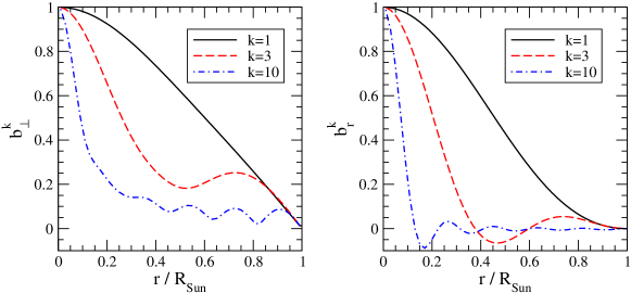
Figure 1: Perpendicular (left), $b_{\perp}^{k}=\sqrt{(b_{\theta}^{k})^{2}+(b_{\phi}^{k})^{2}}$, and radial (right panel), $b_{r}^{k}$, components of modes $k=1,3,10$ of the self-consistent B-field Eq. (5).

Note that such low order modes of the large-scale magnetic field Eq. (5), $k=1,2,\dots 10$, survive against magnetic diffusion over the solar age, $\sim 4.6$ Gyr (Miranda et al., 2001).

Substituting the background magnetic field in Eq. (5) into Eq. (2) one gets all components of the perturbative field ${\bf B}^{{}^{\prime}}(r,\theta,\phi)$, as follows:

$$B_{r}^{{}^{\prime}}=\frac{B_{core}}{R_{\odot}}\left(\frac{\sin\theta\partial_{\theta}Y_{l}^{m}}{x}\left[\xi_{r}(x)b_{\theta}(x)+\xi_{h}(x)b_{r}(x)\right]+\right.$$

$$\left.+Y_{l}^{m}\xi_{r}(x)\left[\frac{imb_{\phi}(x)}{x}-\cos\theta\left(\frac{\partial b_{r}(x)}{\partial x}+\frac{2b_{r}(x)}{x}\right)\right]+\frac{l(l+1)\cos\theta Y_{l}^{m}}{x}b_{r}(x)\xi_{h}(x)\right),$$

$$B_{\theta}^{{}^{\prime}}=\frac{B_{core}}{R_{\odot}}\left(\cos\theta\partial_{\theta}Y_{l}^{m}\left[b_{r}(x)\frac{\partial\xi_{h}(x)}{\partial x}-\frac{\xi_{h}(x)}{x}\left(b_{\theta}(x)+b_{r}(x)\right)\right]+\frac{im\partial_{\theta}Y^{m}_{l}}{x}\xi_{h}b_{\phi}-\right.$$

$$\left.-\sin\theta Y_{l}^{m}\left[\frac{b_{\theta}\xi_{r}}{x}+\frac{\partial(b_{\theta}(x)\xi_{r}(x))}{\partial x}\right]+b_{\theta}\sin\theta\left[\frac{\xi_{h}}{x}\left(\partial^{2}_{\theta}Y_{l}^{m}+l(l+1)Y_{l}^{m}\right)\right]\right),$$

$$B^{{}^{\prime}}_{\phi}=\frac{B_{core}}{R_{\odot}}\left(im\cot\theta Y_{l}^{m}\left[b_{r}\frac{\partial\xi_{h}}{\partial x}-\frac{\xi_{h}}{x}\left(2b_{\theta}+b_{r}\right)\right]+im\frac{b_{\theta}\xi_{h}}{x}\partial_{\theta}Y_{l}^{m}-\right.$$

$$\left.-\sin\theta Y_{l}^{m}\left[\frac{\partial(\xi_{r}(x)b_{\phi}(x))}{\partial x}+\frac{\xi_{r}b_{\phi}}{x}\right]+\frac{\sin\theta b_{\phi}\xi_{h}}{x}\left[l(l+1)Y_{l}^{m}+\frac{1}{\sin^{2}\theta}\frac{\partial^{2}Y}{\partial\phi^{2}}\right]\right)~{}.$$ (8)

Using displacement eigenfunctions $\xi_{r}^{(nl)}(x)$, $\xi_{h}^{(nl)}(x)$ for the g-modes of the order $n$ and degree $l$ (Mathur, Turck-Chièze & Couvidat, 2006) we are able to calculate the perturbative magnetic field ${\bf B}^{{}^{\prime}}(r,\theta,\phi)$ given by Eq. (2) and then the integrals in the initial Eq. (1). This way we obtain the magnetic shift of eigenfrequencies.

3 JWKB approximation

In order to simplify Eq. (1) we adopt the JWKB well-known approximation (Christensen-Dalsgaard, 2003) (see eqs. (7.129)-(7.131) there). This holds for large orders $n\gg 1$ and correspondingly $\omega\ll N$ ($N$ is the Brunt-Väisälä frequency). The resulting g-mode eigenfunctions $\xi_{h}^{(nl)}$, $\xi_{r}^{(nl)}$ of oscillations within RZ are given by

$$\xi_{r}\simeq A\rho^{-1/2}r^{-3/2}\left(\frac{N^{2}}{\omega^{2}}-1\right)^{-1/4}\cos\left[\int_{r_{1}}^{r}\frac{L}{r^{{}^{\prime}}}\left(\frac{N^{2}}{\omega^{2}}-1\right)^{1/2}dr^{{}^{\prime}}-\frac{\pi}{4}\right],$$ (9)

$$\xi_{h}\simeq-A\rho^{-1/2}L^{-1}r^{-3/2}\left(\frac{N^{2}}{\omega^{2}}-1\right)^{+1/4}\sin\left[\int_{r_{1}}^{r}\frac{L}{r^{{}^{\prime}}}\left(\frac{N^{2}}{\omega^{2}}-1\right)^{1/2}dr^{{}^{\prime}}-\frac{\pi}{4}\right],$$ (10)

where $L=\sqrt{l(l+1)}$ and the JWKB connection ${\rm d}\xi_{r}/{\rm d}r\simeq L^{2}\xi_{h}/r$ was used in obtaining $\xi_{h}$.

Obviously, the ratio between the amplitudes of the horizontal and vertical displacements obeys (see Eq. (7.132) in (Christensen-Dalsgaard, 2003)):

$$\left|\frac{L\xi_{h}}{\xi_{r}}\right|\sim\left(\frac{N^{2}}{\omega^{2}}-1\right)^{1/2}.$$

showing explicitly that for low degrees $l=1,2$ the g-mode oscillation is predominantly in the horizontal direction, $\xi_{h}\gg\xi_{r}$. Moreover, differentiating the horizontal component once more, $\partial\xi_{h}/\partial r$, one finds that $\partial\xi_{h}/\partial r\gg\xi_{h}/r$, since the additional large factor $[(N/\omega)^{2}-1]^{1/2}\gg 1$ appears.

We see that the large derivatives $\partial\xi_{h}/\partial x$ enter only in the angular components $B_{\theta}^{{}^{\prime}}$ and $B_{\phi}^{{}^{\prime}}$ given by Eq. (2), which with the angular factors ($\cos\theta\partial_{\theta}Y$) and ($\cot\theta Y$) respectively. As a result, as in Ref. (Hasan, Zahn & Christensen-Dalsgaard, 2005), the dominant term in the integrand of the numerator in Eq. (1) is the first one

$$-[(\nabla\times{\bf B}^{{}^{\prime}})\times{\bf B}]\cdot\vec{\xi}^{*}=\left|{\bf B}^{{}^{\prime}}\right|^{2}\simeq\left(\frac{B_{core}}{R_{\odot}}\right)^{2}\left|\frac{1}{x}\frac{{\rm d}(xb_{r}\xi_{h})}{{\rm d}x}\right|^{2}\left[\left|\cos\theta\frac{\partial Y}{\partial\theta}\right|^{2}+m^{2}\left|\cot\theta Y\right|^{2}\right].$$

The second term in the numerator in Eq. (1) is negligible since it is linear in ${\rm d}\xi_{h}/{\rm d}x$ (in contrast the first term is quadratic). Finally, the leading contribution to the denominator is $\xi_{h}^{2}$, since $\xi_{h}\gg\xi_{r}$ for $n\gg 1$.

Under the above approximations we finally obtain the magnetic shift of g-mode frequencies in the Sun, as

$$\frac{\delta\omega}{\omega}=\frac{C_{lm}(B_{core})^{2}}{8\pi\omega^{2}\rho_{c}R_{\odot}^{2}}\frac{\int\left|x^{-1}{\rm d}(xb_{r}\xi_{h})/{\rm d}x\right|^{2}x^{2}{\rm d}x}{\int\left|\xi_{h}\right|^{2}(\rho/\rho_{c})x^{2}{\rm d}x}=S_{c}\left(\frac{B_{core}}{{\rm MG}}\right)^{2}.$$ (11)

Notice that, in contrast to the 1-D case, here there is a dependence on the angular degree $l$ and azimuthal number $m$. This induces a splitting (not only a shift) of the g-mode frequencies. Note also that this expression is in full agreement with the magnetic shift derived in (Hasan, Zahn & Christensen-Dalsgaard, 2005) for the g-mode spectra in slowly pulsating B-stars. Moreover, the coefficient $C_{lm}$ corresponding to the angular integration coincides exactly with those of Ref. (Hasan, Zahn & Christensen-Dalsgaard, 2005). Notice however, that this coincidence was not expected a priori since here we adopt a self-consistent background magnetic field (Kutvitskii & Solov’ev, 1994) instead of an arbitrary ansatz for $b(x)$, as in Ref. (Hasan, Zahn & Christensen-Dalsgaard, 2005).

In order to compute the magnetic shift we perform the numerical integration in Eq. (11) using the SSeM eigenfunctions $\xi_{r,h}^{(nl)}$ (Mathur, Turck-Chièze & Couvidat, 2006) shown in Fig. 2.

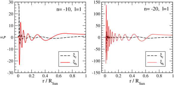
Figure 2: Horizontal $\xi_{h}$ and radial $\xi_{r}$ eigenfunctions as a function of normalized radius, $r/R_{\odot}$, are shown for modes $g_{10}^{1}$ (left) and $g_{20}^{1}$ (right) panel.

Our results are given in Table 1. These results for the magnetic shifts of the g-mode frequencies in the Sun for $g_{10}^{1}$ and $g_{20}^{1}$. One finds that magnetic shifts of the magnitude hinted by the data (order 1%) can be obtained for RZ magnetic field strength 300 ${\rm kG}$ for the mode $g_{20}^{1}$ and 2500 ${\rm kG}$ for the mode $g_{10}^{1}$. We also give the corresponding values of the $S_{c}$ coefficient in Eq. (11). Note that the case of young B-star considered in (Hasan, Zahn & Christensen-Dalsgaard, 2005) one obtains 110 ${\rm kG}$ and 1100 ${\rm kG}$ respectively.

Table 1: Solar RZ magnetic field which would produce a frequency of 1% for g-modes $g_{20}^{1}$ and $g_{10}^{1}$. The magnetic field mode $k=1$ is assumed. See text.

Mode	$\nu$ ($\mu$Hz)	P (hour)	$S_{c}$ (MG-2)	$B_{core}$ (MG)
$g_{20}^{1}$	33.19	8.37	$1.25\times 10^{-1}$	0.28
$g_{10}^{1}$	63.22	4.39	$1.63\times 10^{-3}$	2.48

Note that for low order g-mode candidates, e.g. $g_{3}^{2}$, ($n=-3$, $l=2$, $\nu_{3}^{2}=222.02~{}\mu$Hz) the JWKB approximation is not applicable and, moreover, the RZ magnetic field strengths required to provide the magnetic shift $\sim$ 1% would be huge, hence outside our assumptions.

4 Rotation-induced splitting of g-modes

Here we give the standard estimate of the rotational splitting of the g-mode frequencies obtained in the absence of magnetic field (Christensen-Dalsgaard, 2003). The exact result reads,

$$\delta\omega_{nlm}=m\frac{\int_{0}^{R}\Omega(r)[\xi_{r}^{2}+L^{2}\xi_{h}^{2}-2\xi_{r}\xi_{h}-\xi_{h}^{2}]r^{2}\rho{\rm d}r}{\int_{0}^{R}[\xi_{r}^{2}+L^{2}\xi_{h}^{2}]r^{2}\rho{\rm d}r}.$$ (12)

where the last two terms in the numerator come from the Coriolis force contribution.

For high order g-modes, $n\gg 1$, for which JWKB approximation is valid, $\xi_{h}\gg\xi_{r}$, and assuming rigid rotation of the RZ, $\Omega={\rm constant}$, one obtains the simple 3D formula:

$$\delta\omega_{nlm}=m\beta_{nl}\Omega,$$ (13)

where the last term in the coefficient $\beta_{nl}=1-[l(l+1)]^{-1}$ is given by the Coriolis force contribution.

For the lowest degree $l=1$ this gives $\beta_{nl}=1/2$ while for a high degree $l\gg 1$ the Coriolis term is negligible and $\beta_{nl}=1$. Choosing $\Omega/2\pi=430$ nHz ($T=27$ d) we see from the Table 2 that the JWKB approximation given by Eq. (13) (fourth column) is in good agreement with the exact calculations using Eq. (12) and given in the last column.

Table 2: Here we assumed $\Omega=430$ nHz.

			JWKB, 3D	3D
Mode	$\nu$ ($\mu$Hz)	P (hour)	$\delta\omega/\omega$	$\delta\omega/\omega$
			$\times m\,10^{-3}$	$\times m\,10^{-3}$
$g_{1}^{1}$	263.07	1.05	$0.82$	$0.95$
$g_{3}^{2}$	222.46	1.25	$1.61$	$1.54$
$g_{4}^{1}$	128.34	2.17	$1.68$	$1.64$
$g_{10}^{1}$	63.22	4.39	$3.40$	$3.63$
$g_{10}^{2}$	103.29	2.69	$3.47$	$3.57$
$g_{20}^{1}$	33.19	8.37	$6.48$	$6.60$
$g_{20}^{2}$	55.98	4.96	$6.40$	$6.44$

5 Discussion

Recent observations of g-mode candidates in the GOLF experiment (Turck-Chièze et al., 2004) indicate shifts in the g-mode frequencies corresponding to low order modes that may be as large as $\sim$ 1%, e. g. $g_{1}^{1}$, $g_{3}^{2}$. For such modes the expected rotation splittings seem rather small. We have found that $\delta\omega(\mathrm{rotation})/\omega\sim m\times 0.001-0.0015$ for a flat rotation in the radiative zone. As result rotation cannot provide the frequency shift hinted by GOLF observations for these modes. Nevertheless as the rotation in the core can be slightly increased by a factor greater than 2, it remains important to properly determine the centroid of the observed modes. Moreover, it is important to go beyond the standard model picture and introduce the effect of transport and mixing in the solar radiative zone which may also impact on the prediction of the high frequency gravity modes.

Here we mainly study that such shifts may result from RZ magnetic fields. In order to give an estimate of the corresponding values of RZ magnetic fields we have adopted the standard 3-D MHD JWKB perturbative approach, aware that its validity is limited to relatively large modes. We have found that the magnetic shift of g-mode frequencies for high order modes $\delta\omega/\omega\sim B_{core}^{2}/\omega^{2}$ can be of order 1% for realistic central magnetic fields values obeying all known upper bounds discussed in the literature. For example, we have obtained magnetic fields $B_{core}\simeq 300~{}{\rm kG}$ and $B_{core}\simeq 2500~{}{\rm kG}$ for $g_{20}^{1}$ and $g_{10}^{1}$, respectively. Such values are in qualitative agreement with recent calculated magnetic field values 110 ${\rm kG}$ and 1100 kG providing magnetic shift 1% for the same modes in the case of young $4~{}M_{\odot}$ B-stars (Hasan, Zahn & Christensen-Dalsgaard, 2005). Future observations of such high order g-modes $n\gg 1$ in the Sun could shed light on the validity of our assumption. In fact we have already some signature of these modes obtained from their asymptotic properties. However, due to their very low amplitudes, we have presently mainly analyzed the sum of dipole gravity modes from $n=-4$ to $-26$ (Garcia et al., 2006). A proper decomposition of the observed waves will place more constraints on the shift of these modes.

In contrast, to consider the case of low order modes hinted by the recent GOLF data requires further assumptions. In order to provide estimates for this case we consider two approximations. First we recall the general dependence $\delta\omega/\omega\sim B_{core}^{2}/\omega^{2}$. It implies that, in order to provide the same magnetic shift $\sim$ 1% the magnetic field for modes $g_{1}^{1}$, $g_{3}^{2}$ should be much stronger than in the case of JWKB frequencies, $n\gg 1$. E.g. for the g-mode candidate $g_{3}^{2}$ with $\nu=222.46~{}\mu$Hz (Turck-Chièze et al., 2004) from the frequency ratio $\nu(g_{3}^{2})/\nu(g_{10}^{1})=222.46/63.22=3.52$, one finds that the magnetic field which provides a shift $\sim$ 1% for $g_{3}^{2}$ would be $\sim 8.8$ MG. Such large RZ magnetic field estimate also agrees with the 1-D MHD approach given in Ref. (Rashba, Semikoz & Valle, 2006) (although such 1-D picture can not provide angular splittings, it has the merit of not relying on the JWKB approximation). Indeed, such trend for low order modes, $n=-3,-2,-1$, is seen in Fig. 4 of Ref. (Rashba, Semikoz & Valle, 2006) taking into account that the transversal wave number parameter ${\rm k=2}$ of the 1-D approach is analogous to the degree $l$ in the 3-D approach and 2.8 times more magnetic field value for the maximum Brunt-Väisälä frequency approximated as $N=2.8\times 10^{-3}~{}{\rm rad/sec}=constant$ instead of $\sim 10^{-3}~{}{\rm rad/sec}$ applied in numerical calculations in (Rashba, Semikoz & Valle, 2006).

The possible existence of such strong magnetic fields in the RZ is somewhat disturbing. It could be that neither rotation, nor magnetic fields are responsible for the hinted frequency shift with respect to SSeM prediction. For example, the $g_{3}^{2}$ mode might mix with other gravity modes penetrating RZ with frequencies just below Brunt-Väisälä frequency.

In this paper we have considered the possibility of a 1% magnetic shift of eigenfrequencies, independently of the frequency considered. The sensitivity to the detailed physics depends on the order of the mode as shown in (Mathur, Turck-Chièze & Couvidat, 2006) and is greater at high frequency (low order) than at large order, demonstrating the great interest of these modes.

The effect of the magnetic field on the frequency shift is expected to depend on its shape. In a forthcoming paper we plan to explore the sensitivity of magnetic shifts of g-modes in the Sun to the structure of magnetic fields given by the self-consistent MHD model. Indeed, refined g-mode data may enable future tomography studies of the structure of RZ magnetic fields.

In short, the search for fundamental solar characteristics deep within radiative zone constitutes an important challenge for helioseismology methods. Here we have given a conservative limit on the magnitude of the magnetic field obtained from its possible effect on the g-mode frequencies. Alternatively, the propagation of neutrinos may probe short-wave MHD density perturbations in the solar RZ ($\lambda_{MHD}\sim 100-200~{}{\rm km}$) as already discussed in Refs. (Burgess et al., 2003, 2004a, 2004b).

References

- Burgess et al. (2003) Burgess, C.P. et al., 2003 , ApJ, 588, L65
- Burgess et al. (2004a) Burgess, C.P. et al., 2004a, MNRAS, 348, 609
- Burgess et al. (2004b) Burgess, C.P. et al., 2004b, JCAP, 01, 007
- Christensen-Dalsgaard (2003) Christensen-Dalsgaard, J., 2003, Lecture Notes on Stellar Oscillations, available at http://astro.phys.au.dk/~jcd/oscilnotes/
- Couvidat, Turck-Chièze & Kosovichev (2003) Couvidat, S., Turck-Chièze, S., Kosovichev, A.G., 2003, ApJ, 599, 1434
- Garcia et al. (2006) Garcìa, R. et al., Science, 2007, in press
- Hasan, Zahn & Christensen-Dalsgaard (2005) Hasan, S.S., Zahn J.-P. & Christensen-Dalsgaard, J. 2005, A&A 444, L29
- Kutvitskii & Solov’ev (1994) Kutvitskii, V.A., Solov’ev L.S., 1994, JETP, 78 (4), 456-464 (In Russian Zh. Eksp. Teor. Fiz. 105, 1994, 853-867)
- Mathur, Turck-Chièze & Couvidat (2006) Mathur, S., Turck-Chièze, S., Couvidat, S. & Garcìa, R., 2007, ApJ, submitted
- Miranda et al. (2001) Miranda, O.G., et al., 2001, Nucl.Phys., B595, 360-380
- Moss (2003) Moss, D. 2003, A&A, 403, 693
- Ruzmaikin & Lindsey (2002) Ruzmaikin, A., & Lindsey, C. 2002, in Proceedings of SOHO 12/GONG + 2002 “Local and Global Helioseismology: The Present and Future”, Big. Bear Lake, California (USA)
- Rashba, Semikoz & Valle (2006) Rashba, T.I., Semikoz, V.B., Valle, J.W.F., 2006, MNRAS, 370, 845-850
- Turck-Chièze et al. (2001) Turck-Chièze, S. et al., 2001, ApJ, 555, L69
- Turck-Chièze et al. (2004) Turck-Chièze, S., et al. 2004, ApJ, 604, 455
- Unno et al. (1989) Unno, W., Osaki, Y., Ando, H., Saio, H., and Shibahashi, H. 1989, Nonradial Oscillations of Stars, 2-nd edition (Univ. of Tokyo Press, Tokyo)