Synthetic Mid-UV Spectroscopic Indices of Stars

Abstract

Using the UVBLUE library of synthetic stellar spectra we have computed a set of mid-UV line and continuum spectroscopic indices. We explore their behavior in terms of the leading stellar parameters ($T_{\mathrm{eff}}$, $\log{g}$). The overall result is that synthetic indices follow the general trends depicted by those computed from empirical databases. Separately we also examine the index sensitivity to changes in chemical composition, an analysis only feasible under a theoretical approach. In this respect, lines indices Fe i 3000, BL 3096 and Mg i 2852 and the continuum index 2828/2921 are the least sensitive features, an important characteristic to be taken into account for the analyses of integrated spectra of stellar systems. We also quantify the effects of instrumental resolution on the indices and find that indices display variations up to 0.1 mag in the resolution interval between 6–10 Å of FWHM. We discuss the extent to which synthetic indices are compatible with indices measured in spectra collected by the International Ultraviolet Explorer (IUE). Five line and continuum indices (Fe i 3000, 2110/2570, 2828/2921, S2850, and S2850L) display a remarkable good correlation with observations. The rest of the indices are either underestimated or overestimated, however, two of them, Mg Wide and BL 3096, display only marginal discrepancies. For 11 indices we give the coefficients to convert synthetic indices to the IUE system. This work represents the first attempt to synthesize mid-UV indices from high resolution theoretical spectra and foresees important applications for the study of the ultraviolet morphology of old stellar aggregates.

1 Introduction

With the accessibility to the rest-frame mid-ultraviolet (2200–3200 Å) spectra of distant evolved systems ($0.5<z<2.0$), the analysis of the ultraviolet morphology of intermediate and late type stars and old systems in the local universe has regained interest (e.g. Spinrad et al., 1997; Nolan, Dunlop, & Jimenez, 2001; and, more recently, McCarthy et al., 2004; Cimatti et al., 2004). Dating galaxies which have gone through null or negligible star formation events over the past few Gigayears at these redshifts has fundamental implications not only from an individual object point of view, but also at cosmological scales.

The mid-ultraviolet offers a new spectral window which may help to break the so-called age-metallicity degeneracy present in the optical spectra of evolved stellar systems (Worthey, 1994; Buzzoni, 1995; Jimenez et al., 2004). In general, the UV analyses of stellar populations have relied on empirical stellar databases, mainly the one constructed upon IUE low resolution data (Wu et al., 1983). Among the most important efforts to characterize the UV morphology of stars that presumably dominate the UV spectrum of old systems was presented by Fanelli, O’Connell, & Thuan (1987) and Fanelli et al. (1990, 1992). They have defined 25 narrow-band indices in the ultraviolet covering two spectral segments: 1230–1930 Å and 1950–3200 Å, corresponding to the wavelength limits of IUE cameras. Spectroscopic indices defined in the far-UV (Fanelli et al., 1987) were created to provide alternative tools for the analysis of active star-forming galaxies. The second set of indices (Fanelli et al., 1990) was constructed with the aim of analyzing the properties of prominent spectral features in old populations. In general, these indices focus on wavelength regions that are more sensitive to stellar atmospheric parameters and less affected by the IUE instruments artifacts and by the effects of features (emission and/or absorption) of interstellar origin. Given the prevailing contribution to the mid-UV wavelength range of bright main sequence stars (O’Connell, 1999; Buzzoni, 2002), the study of this spectral region is of special importance as a diagnostic tool, for instance to date high-redshift galaxies (Heap et al., 1998).

It has been recognized, however, that empirical databases are generally composed of stars of the solar neighbourhood and therefore unavoidably carry on the evolutionary imprints of the Milky Way. In order to cope the paucity of chemical composition of empirical libraries required for the analysis of old stellar systems, many of the population synthesis works have incorporated theoretical libraries of stellar fluxes. Amongst the most popular libraries is the Kurucz grid of spectral energy distributions (SEDs) which is public through his web site. It has been found that Kurucz flux library well represents segments of the mid-UV spectra of stars of intermediate and late type, in particular the continuum measurements (slopes in the SEDs) and some features such as the blend at about 2538 Å (LFB00). The limitations of the public Kurucz grid of fluxes has been a matter of discussion in several investigations. In this respect Dorman, O’Connell, & Rood (2003) concluded that for the analysis of the integrated UV properties of stellar aggregates, low resolution synthetic fluxes should be preferred over high resolution data. The reason being that use of high resolution theoretical data is precluded by the still unsolved uncertainties in atomic and molecular line data. It is important to note, nevertheless, that Kurucz grid of fluxes have a wavelength sampling of 10 Å and therefore might lack of the appropiate resolution for a direct comparison with, for example, the commonly used IUE database.

While we agree that, for now, only low resolution (e.g. broad band indices) can be safely used, it is important to stress that at low resolution a great deal of information is lost and efforts should concentrate in the improvement of high resolution theoretical data. Such an improvement must be based on a quantitative validation process by comparing theoretical data with stellar observations. On this line, Peterson et al. (2001, 2003) and Peterson (2005) have embarked into a project aimed at providing a large theoretical database fully consistent with Space Telescope Imaging Spectrograph (STIS) observations.

In this paper we present a quantitative comparison between observed mid-UV features in the form of absorption line and continuum indices and those computed from high resolution synthetic spectra. We start, in Section 2, by investigating the effects of stellar parameters and instrumental resolution on spectroscopic indices from a purely theoretical point of view. In Section 3 we compare theoretical and observed indices and discuss the extent to which empirical indices are reproduced by theory. Section 4 is devoted to provide the equations needed to transform theoretical (discrepant) indices to the standard (IUE) system. This represents the first attempt to derive synthetic indices from high resolution mid-UV spectra.

2 Theoretical UV indices

Following the definitions given in Table 1, we carried out the calculation of a set of mid-ultraviolet indices of the synthetic stellar SEDs of the UVBLUE library, described in Rodríguez-Merino et al. (2005, hereafter Paper I). The indices measure either the strength of absorption features or the slope of the continuum. It is important to mention that most of the definitions listed in Table 1 correspond to those provided by Fanelli et al. 1990. Two continuum indices (S2850 and S2850L) are analogous to the index defined by LFB00. The band passes for these two indices and for 2110/2570 are those of Bressan (private communication). In column 5 of Table 1 we list the atomic species that most contribute to the absorption in the central band of each line index. The list has been assembled from a visual inspection of the relevant absorption features present in the theoretical spectrum with $T_{\mathrm{eff}}$/$\log{g}$/[M/H]=5000/4.0/0.0.

The general procedure followed by Fanelli et al. (1990) to define the wavelength sequence and measure spectroscopic indices was carried out in a way similar to that described by O’Connell (1973). For the calculations presented here, UVBLUE has been degraded to match IUE nominal resolution (FWHM=6 Å). The line indices are the ratio of the integrated flux $F_{i}(\lambda)$ in the index passband to the integrated continuum flux $F_{c}(\lambda)$, obtained by linear interpolation of the mean flux of the two side bands; the result is transformed to magnitudes:

$$I=-2.5\times\log_{10}{\frac{\int_{\lambda_{1}}^{\lambda_{2}}{F_{i}(\lambda)\,d\lambda}}{\int_{\lambda_{1}}^{\lambda_{2}}{F_{c}(\lambda)\,d\lambda}}}\,,$$ (1)

where $\lambda_{1}$ and $\lambda_{2}$ are the limits of the index passband.

The continuum indices are given by the ratio of the mean flux of the blue passband, $\overline{F}_{b}(\lambda)$, to the mean flux of the red one, $\overline{F}_{r}(\lambda)$, transformed to magnitudes:

$$I=-2.5\times\log_{10}{\frac{\overline{F}_{b}(\lambda)}{\overline{F}_{r}(\lambda)}}\,.$$ (2)

In the mid-UV, the spectra of intermediate and late-type stars are strongly affected by line blanketing and therefore it is hard to find spectral regions free from features. For this reason the spectral bands are selected such as to optimize each index for a temperature interval in which the feature is maximum.

The homogeneous coverage in stellar parameters, in particular the chemical composition, allows the investigation of their effects on each index. The results are partially presented in Table 2 where we list some synthetic indices (line indices) for a subset of atmospheric parameters in UVBLUE, identified in columns 1-3. The full grid of indices is avaliable in electronic form. In Figure 1 we plot the index vs. effective temperature ($T_{\mathrm{eff}}$) and surface gravity ($\log{g}$) for synthetic spectra of solar metallicity. The reference labels inscribed in the upper left panel stand for different gravities which range from $\log{g}=0.0$ to 5.0 dex. We would like to stress at this point that the approach in this section is purely theoretical and not meant to analyze the compatibility between theoretical and empirical indices.

Some general remarks can be drawn just on the basis of a quick-look analysis of the different plots of Fig. 1, simply relying on prime physics principles. In all cases it is evident that indices probe a characteristic temperature range at which the corresponding absorption feature (or pseudo-continuum break) is maximum. As expected, metal indices for higher ionization states generally peak at warmer effective temperature: this is because stellar layers at the appropriate thermodynamical conditions to produce the feature lie at a shallower optical depth with increasing stellar effective temperature. This is well evident, for instance, looking at the Mg ii 2800 and Mg i 2852 indices or comparing the Fe ii 2402 feature with the Fe i 3000 one. In both cases, the higher ionization state is the prevailing one among F stars while the neutral metal becomes more important for the G spectral type.

As for gravity effects, one has to consider that the relative partition of a given elemental species between, let us say, first ($X_{\sc II}$) and neutral ($X_{\sc I}$) ionization states scales according to the Saha equation (e.g. Mihalas, 1978) as

$${X_{\sc II}\over X_{\sc I}}\propto{{T^{3/2}e^{-1/kT}}\over P_{e}}.$$ (3)

with $P_{e}$ being the electronic pressure of the stellar plasma.

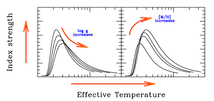
Figure 2: The expected effect on metal indices by increasing electronic pressure ($P_{e}$) in stellar atmosphere. This effect can be induced either by increasing surface gravity $\log g$ (that is by “packing” atoms more efficiently) or by increasing metal abundance (thus increasing the main $e^{-}$ donors to the plasma). Note the different trend of the index strength depending whether gravity or metallicity are acting. In the first case (left panel) we expect a weaker index for dwarf stars compared to giants due to the wiping effect of damping broadening in the spectral features with increasing gravity. Conversely (right panel), the index tends to be stronger if we increase the corresponding elemental abundance.

Therefore, with increasing $\log g$ (that is by “packing” atoms more efficiently) one makes easier the ionization process allowing metals to more efficiently feed $e^{-}$ to the plasma. As a consequence, the correspondingly higher value of $P_{e}$ leads any given equilibrium partition $X_{\sc II}/X_{\sc I}$ to shift to slightly higher temperatures. So, in Fig. 1 a given spectral feature is seen to peak at earlier spectral types with increasing $\log g$ (see, for instance, the nice trend of Fe ii 2402 or Mg ii 2800 in the figure). In addition, the broader damping wings of high-gravity spectral features mimic the wiping effect of a lower spectral resolution (see Sec. 2.2) thus favoring weaker index values for dwarf stars compared to giants. These qualitative arguments are summarized in Fig. 2.

Based on a more careful inspection of Fig. 1, we can give below further comments on individual indices:

Fe ii 2332: the absorption in the central band of this index is mainly due to Fe ii and Fe i lines, although several other elements add significant contribution, as in all other indices that we present here. This index has its maximum for all gravities at about $T_{\mathrm{eff}}=6000$ K. It displays a large variation with surface gravity, ranging from 0.5 mag for high gravity stars to 1.5 mag for supergiant spectra.

Fe ii 2402: feature produced by multiplets of Fe ii. This index is very sensitive to gravity. At its maximum, at $T_{\mathrm{eff}}=6000$ K, the index doubles its value from about 0.8 to 1.5 mag when the gravity decreases from $\log{g}=5.0$ to 1.0. All gravities peak at about the same temperature (6000 K).

BL 2538: the blend is produced by mainly Fe, Mg, Cr, and Ni absorption. Among line indices, BL 2538 shows the highest sensitivity to surface gravity. It peaks (index $\approx 1.5$ mag) at the lowest temperature (4000 K) for $\log{g}=5.0$. For $\log{g}=0.0$ the index drastically drops to negative values. Note that, contrary to most indices, for $T_{\mathrm{eff}}$ above 4500 K this index increases with increasing gravity.

Fe ii 2609: the absorption in the index band is largely due to Fe ii, with contributions by Fe i and Mn ii. This index has its maximum at about 5000 K, temperature at which it displays a strong sensitivity to gravity with a variation from 1.5 mag, for $\log{g}=5.0$, to 2.5 mag for $\log{g}=2.0$. It peaks at about the same temperature for all gravities.

BL 2720: blend produced by neutral and ionized iron lines, with presence of Cr i and V ii. Down to $T_{\mathrm{eff}}=4500$ K, this index shows little variation with surface gravity, with the exception of the outermost $\log{g}$ values. Similarly to BL 2538 for high gravity, this index reaches its maximum at the lowest temperatures.

BL 2740: blend of iron and chromium lines. This index is similar to BL 2720 in that it shows marginal dependence with gravity, it sharply increases with decreasing $T_{\mathrm{eff}}$, and it peaks at the lower temperature edge of UVBLUE.

Mg ii 2800: this index includes the strongest feature in the mid-UV interval, due to Mg ii. It sharply increases shortward of 10000 K and peaks at about 6000 K for $\log{g}=5.0$ and 5000 K for $\log{g}=0.0$. The index shows slight dependence on gravity since it varies about 30% along the full gravity interval. This dependence is restricted for $T_{\mathrm{eff}}<6000$ K.

Mg i 2852: this index is produced by a strong Mg i absorption line. It displays an enhanced sensitivity to the surface gravity with respect to Mg ii 2800. Indices from high gravity spectra peak at $T_{\mathrm{eff}}=6000$ K, while for the lowest gravity the maximum value is reached at about 4500 K.

Fe i 3000: the absorption in the index band is dominated by Fe i. It appears to be sensitive to $T_{\mathrm{eff}}$ in a short range, $4000\leq T_{\mathrm{eff}}\leq 8000$ K, and it is moderately dependent on gravity.

BL 3096: the blend is produced by Fe i, Ni i, Mg i, and Al i. It displays a marginal sensitivity on gravity for high gravity spectra. Giants and supergiants are not separated among themselves.

Mg Wide : this index covers 600 Å of the mid-UV SED. Its central band contains those of BL 2720, BL 2740, Mg ii 2800, and Mg i 2852. Is has been envisaged as a useful indicator of the effective temperature of the dominant stellar population in evolved systems. Defined by three 200 Å-wide bands, this index is expected to be suitable for the analysis of low resolution data of distant galaxies collected by current large facilities (Heap et al., 1998; McCarthy et al., 2004). The curves depicted in Fig. 1 show that the index increases monotonically for most gravities up to the low temperature edge; only for $\log{g}=5.0$ the index saturates at 4500 K (early K-type stars). Mg Wide is very sensitive to surface gravity with indices derived from lower gravity spectra displaying the highest values.

The general behavior of continuum indices (spectral breaks and broad band indices) is depicted below.

2110/2570: this index primarily measures the strong Mg i magnesium break at 2512 Å. It is interesting to note that down to about 5000 K the index is insensitive to gravity. At lower temperatures the effects of gravity are moderate. For synthetic fluxes with $T_{\mathrm{eff}}>7000$ K the index turn to negative values.

2609/2660: as indicated by Fanelli et al. (1990) the spectral break at about 2600 Å is dominated by iron opacity. In our synthetic spectra indices for all gravities peak at about the same temperature (5500 K) with perhaps a slight shift towards lower temperatures at lower gravities. The index shows a moderate sensitivity to gravity, changing by 50% over the entire $\log{g}$ interval. The break vanishes for models of 10000 K.

2828/2921: this break is among the most prominent features in the mid-UV spectra in cool stars and evolved populations. It displays very low sensitivity to surface gravity for model spectra of $T_{\mathrm{eff}}>5000$ K. Below this temperature, which marks the peak for high gravity fluxes ($\log{g}=5.0$), the trends for different gravities clearly separate. At the lowest temperatures the change of the index in the interval $\log{g}=0.0$–5.0 is about a factor of two.

2600-3000, S2850, and S2850L: as can be seen from the bands listed in Table 1, these indices measure the slope between 2600 and 3000 Å. The differences are the band widths and the centers of the bands of the index 2600-3000. As expected, the overall behavior of the three continuum indices is very similar: all turn from negative to positive values at $T_{\mathrm{eff}}\sim 10000$ K, higher gravity model fluxes display larger indices, and all are sensitive to gravity, with an enhanced sensitivity of the index S2850 that varies almost a factor of three from $\log{g}=0.0$ to 5.0.

We have described the general behavior of the 17 line and continuum indices from a purely theoretical point of view. It is worth to remark that the above results are affected by the theoretical limitations of model atmospheres, in particular, the limitations inherent to models constructed under the classical approximations, as is our case. In Paper I we have commented on the UVBLUE caveats and the reader is referred to that paper for more details. The discussion of the impact of UVBLUE limitations on synthetic indices is deferred to Sec. 3. Nevertheless, we can anticipate that the overall trends of index values with $T_{\mathrm{eff}}$ and surface gravity are similar to those depicted by indices computed from empirical data (Fanelli et al., 1992). Note that we have restricted the analysis to line indices redward of 2300 Å since both, theoretical and observed spectra, decrease in quality for intermediate and late stellar types. In what follows we describe the effects of chemical composition, which, in the context of stellar populations analyses, might be more important than those of gravity.

2.1 Effects of metallicity

The uniform metallicity coverage of UVBLUE (from [M/H]=$-$2.0 to $+0.5$) allows the investigation, at least from an exploratory point of view, of the effects of chemical composition on spectroscopic indices. Such an investigation is not feasible with current empirical databases since the vast majority of objects have solar or nearly solar metallicity (see Fig. 8 of Paper I).

In Fig. 3 we show the trends of the mid-UV spectral indices as a function of the effective temperature and metallicity for a fixed surface gravity of $\log{g}=4.0$ dex. Different line types correspond to different metallicities as denoted in the labels in the upper left panel in the figure. Like for gravity effects, a similar trend on spectrophotometric indices has also to be expected by increasing stellar metallicity. In this case, $P_{e}$ would increase in eq. (3) merely as a consequence of a higher value of $Z$. In addition, in case of thin absorption features, the corresponding index strength would increase reaching a stronger peak for higher values of metal abundance. This is nicely shown in Fig. 3, specially for the case of metal blends, like the BL 2538 or BL 2740 indices.

Recalling our previous physical arguments (see right panel of Fig. 2), note that systematically, the loci of the maxima in the plots of Fig. 3 also depend on the metal content, this is, high metallicity indices peak at higher temperatures. Because of this, in some indices, namely Fe ii 2332, Fe ii 2402, and Mg ii 2800, the effects of chemical composition are reversed after the index saturates towards low $T_{\mathrm{eff}}$: at the lowest temperatures the low metallicity indices are higher. The peak at different metallicities are shifted by as much as 3000 K if we compare, for the index Fe ii 2402, metal rich indices with those of the lowest chemical composition. The variation of the indices can be as high as a factor of three in the full metallicity interval.

The three redder indices, Mg ii 2852, Fe i 3000, and, notably, BL 3096 display marginal variations with chemical composition. This property seems promising for separating the effects of age and metallicity in integrated spectra.

2.2 Effects of instrumental resolution

An important test that has to be conducted and quite often is neglected is the analisys of sensitivity of spectral indices to instrumental resolution. The comparison of theoretical vs. observed indices (either stellar or integrated) or the analyses of indices measured from spectra from data sets collected with different instrumentation should be carried out with data at the same resolution. The risk of not doing so can be, for instance, the incorrect segregation of potential useful indices. The changes due to spectral resolution might have important implications in the calculation of spectroscopic indices, in particular if the indices are used in the study of the integrated properties of galaxies whose spectra are intrinsically broadened by the motions of the stellar component.

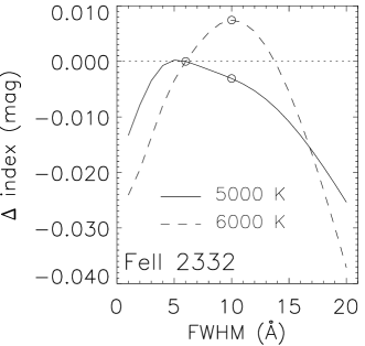
Figure 4: Effects of instrumental resolution of index values. The y-axis indicates the index residual with respect to their value at the nominal IUE resolution (6 Å) illustrated as a horizontal dotted line and an open circle at the 6 Å–0 mag intercept. We have also denoted with an open circle index values at 10 Å resolution compatible to the widely used Kurucz public fluxes. Solid and dashed lines correspond to indices for $T_{\mathrm{eff}}$=5000 and 6000 K synthetic spectra, respectively.

In Figure 4 we show the effects of resolution on the line and continuum indices discussed in the previous section. In the y-axis we indicate the index difference with respect to its value at a resolution of 6 Å. For the analysis we have considered two synthetic spectra of $\log{g}=4.0$, [M/H]$=+0.0$ and $T_{\mathrm{eff}}=5000$ and 6000 K (represented by solid and dashed lines, respectively), temperatures at which most indices reach their maxima. Data points correspond to indices measured in spectra after applying Gaussian filters for differents FWHM ranging from 1 to 20 Å with a step of 1.0 Å. The open circles in each panel indicate the position of the reference IUE resolution (6 Å) and the resolution of the Kurucz public library of fluxes (Kurucz, 1993). In general, one would expect that resolution effects will be modulated by the width of the bands, in the sense that broader bands will be less sensitive to resolution. In a similar way, effects of resolution will depend on the intrinsic width of the spectral lines, this is, whether a line is fully embraced or not within the central bandpass. Let us first comment on the line indices.

We can identify several properties of the effects of resolution on index values. First, all line indices have their lowest value at the lowest resolution (20 Å). The only exception is Mg Wide, which, however, displays a marginal variation of less 0.002 mag between 6 and 10 Å. Second, all indices have their peak values either at the highest resolution or at about 2–4 Å. This is most probably due to the role that features very near to the limit of the bands (either inside and outside) play in modulating an index. Third, with the exception of the index BL 3096, all indices vary up to 40% in the full resolution range. BL 3096 doubles its value from 1 to 20 Å, and changes as much as 0.05 mag (about 20%) in the 6 to 10 Å interval.

Concerning the continuum indices we find a wide diversity of behaviors, nevertheless in four of them (2120/2570, 2600-3000, 2609/2660, and S2850L) the effects of resolution are very weak within the full resolution range, while for the remaning two, 2828/2921 and S2850, values change up to 0.12 mag and 0.8 mag (30 and 40%), respectively. Note that this latter couple of indices are those defined with the narrowest bands. It is important to stress that the exercise shown here is based only on two model spectra. At other temperatures and chemical compositions the effects might decrease or be enhanced.

3 Empirical vs Theoretical Indices

With the goal of quantitatively compare theoretical indices with indices derived from observed data, we have adopted the database described in Paper I to where the reader is referred for more details. In summary, our working sample is based on the Wu et al. (1983) atlas of IUE low resolution spectra and the cool star extension by Fanelli et al. (1990). A sub sample of 111 stars was secured by imposing that at least one full set of atmospheric parameters be available in Cayrel de Strobel et al. (1997).

Keeping in mind that there exist differences in the image extraction processes used in the original Wu et al. (1983) atlas and our IUE-INES data set, we have, as a first step, verified the extent to which new indices measured in re-processed IUE spectra are compatible with those reported by Fanelli et al. (1990). The overall result is that most indices display a one to one correlation with the exception of Fe ii 2402 where there is a quite high dispersion for points corresponding to giant stars. The most plausible explanations for these differences are, on one side, the different absolute flux calibration curves used in INES (González-Riestra et al., 2001) and IUESIPS (Bohlin et al., 1980) and, on the other side, the fact that we used all available images of good quality (in some cases more than 50) while Wu et al. (1983) considered only a few. In addition to this, one has to consider that spectra of cool stars are often quite noisy since their intrinsic UV flux descreases drastically and that at the short wavelength edge the flux is close to the LWP/R cameras sensitivity limits. With the indices computed in the re-processed IUE images we have defined the standard system.

From the theoretical side, we have created a synthetic data set through a three-linear interpolation of the flux, divided by the corresponding $\sigma T_{\mathrm{eff}}^{4}$, of the UVBLUE spectra in the space ($T_{\mathrm{eff}}$, $\log{g}$, [M/H]). For each star we adopt the parameters listed in Table 2 of Paper I. As in the case of the synthetic SEDs presented in the previous section, these spectra were degraded to match IUE resolution (6 Å). It is important to mention that we have imposed one restriction for the comparison: we have excluded low gravity objects ($\log{g}\leq 3.5$) since, on one side, giant and supergiant stars show the largest discrepancies between observed and theoretical SEDs according to Paper I and, on the other side, intrinsic UV fluxes of low gravity objects at the short wavelength edge of IUE are lower that the high gravity counterparts. Additionally, evolved objects of low surface gravity are not expected to significantly contribute to the mid-UV flux of early-type systems, one of the main foreseeable applications of synthetic UV indices. The final sample for our comparison is composed of 68 objects whose distribution in $T_{\mathrm{eff}}$ and [M/H] is displayed in Figure 5. The restriction on wavelength for the material presented in this paper ($\lambda\geq 2300$ Å, except for the spectral break index 2110/2570) ensures a higher signal to noise in observed data. Note also that no restriction on chemical composition was imposed.

The results of the comparison are displayed in Figure 6, where we plot the synthetic indices ($y$-axis) and IUE-indices ($x$-axis) together with a reference 45^∘ dotted line. Ten indices are overestimated by the results of classical model atmospheres. Of these indices two of them (Fe ii 2332 and Fe ii 2402) represent the worst cases with a large scatter over the whole index range. All the remaining overestimated indices (BL 2538, Fe ii 2609, BL 2720, BL 2740, Mg ii 2800, Mg i 2852, BL 3096, and the spectral break 2609/2660) exhibit a clear linear correlation; however, in five of them there is a notable enhancement of scattering on the points for low temperatures stars, not so for the indices BL 2720, Mg i 2852, and BL 3096. Additionally, it is interesting to note that in three indices with large scatter at low $T_{\mathrm{eff}}$ the linear relation appears to be truncated and the empirical indices show a reversal, i.e. indices saturate and decrease after reaching their maxima towards low temperatures. This situation is not modelled by the synthetic indices. Two indices (Mg Wide and the continuum index 2600-3000) appear slightly underestimated by theory. Finally, five indices appear properly reproduced by UVBLUE indices: 2110/2570, Fe i 3000, the spectral break 2828/2921, and the continuum indices S2850 and S2850L.

Let us compare our results with those of Lotz, Ferguson & Bohlin (2000, herefater LFB00) which represent, to our knowledge, the only attempt so far to compare Kurucz-derived synthetic mid-UV indices with observations. They present eight indices all of which are included in our analysis, although, our definition of S2850 is different from that of LFB00. They concluded that for five of these indices, namely, Fe ii 2402, Fe ii 2609, Mg ii 2800, Mg i 2852, and Mg Wide, values are overestimated by Kurucz model fluxes. They found a good match for BL 2538 and for S2850 (the latter for stellar models with $T_{\mathrm{eff}}\geq 4500$ K), while Fe i 3000 is underestimated by 0.15 mag. While our results agree for the first four indices, for the rest we obtain contradicting behaviors. The BL 2538 index appears to be also overestimated, particularly at low temperatures, Mg Wide is somewhat underestimated, and our synthetic Fe i 3000 and the slope between 2600 and 3000 Å match very well empirical indices. There are three plausible explanations for the conflicting results. First, the fact that LFB00 measure theoretical indices from the set of Kurucz model fluxes compiled by Lejeune, Cuisinier, & Buser (1997) which are at a nominal resolution of 10 Å  while our high resolution theoretical data set has been degraded to 6 Å. As we have explained in Section 2.2, this change in resolution can account, at least partially, for the discrepancies. For instance, BL 2538 and Fe i 3000 decrease by about 0.04 mag after changing the resolution from 6 to 10 Å. Second, Kurucz model fluxes are calculated using the opacity distribution functions (ODFs) while the UVBLUE SEDs account for detailed line opacity. It is clear that the statistical nature of the ODFs dilutes the effects of incomplete and/or incorrect line opacities, however, at the price of preventing the possibility of producing spectra at high enough resolution (see also the discussion in Dorman et al., 2003). Third, in our comparison we have accounted for the individual stellar parameters while LFB00 provide a comparison of empirical indices obtained from mean stellar IUE spectra with those measured from a single-gravity single-metallicity (solar) theoretical flux. Even though the definition of the S2850 index in LFB00 and our work differs, our comparison indicates that the slopes we measure in UVBLUE-interpolated spectra closely reproduce empirical results.

Various agents more can be brandished to explain the discrepancies seen in Figure 6. As briefly mentioned by LFB00 and listed in Paper I as caveats of UVBLUE, these are: incomplete line lists, which directly affect the heavily blanketed ultraviolet fluxes; departures from LTE and chromospheric heating. Additionally, and not explicitly mentioned in the above investigations, is the fact that, even if we had a complete line list, the line parameters (mainly the oscillator strengths, Van der Waals damping constants and wavelengths) might be wrong. We believe that discrepancies in many of the indices can be significantly reduced with the improvement of these three parameters, since, as demonstrated in Paper I, individual lines are systematically stronger in theoretical spectra.

3.1 Comments on discrepant indices

A thorough spectral line study and their effects on individual index bands is necessary to unambiguously identify the agent(s) that provoke the discrepancies in the comparison between observed and theoretical indices. Such an analysis is beyond the scope of this work, however, we can speculate on the most likely explanations.

Mg Wide and 2600-3000: the underestimation of these two indices is attributed to a lower opacity in their shared blue band which partially includes the spectral region 2640–2700 Å. In Paper I we have already pointed out that this region is poorly reproduced by model spectra; the most plausible reason for this is the lack of many absorption lines in the UVBLUE line list (Peterson et al., 2001). Furthermore, in UVBLUE we did not considered the so-called “predicted” lines (Kurucz, 1992) which affect the blanketing in this region. The reason for avoiding the use of lines with non-laboratory atomic data is that UVBLUE is also intended for high resolution analyses and the inclusion of unreliable data greatly increases confusion for line identification. Moreover, for Mg Wide these effects are mixed with the overvalued strength of the Mg features comprised in its central band. We do not expect any important contribution to the inconsistencies from the red band since, on one side, we know that within the mid-UV spectral interval line blanketing effects are enhanced towards shorter wavelengths. On the other side, the red and middle bands and partially the blue band of the index Fe i 3000 are embraced by the red band of Mg Wide and 2600-3000, and this index is well reproduced.

Fe ii 2609, BL 2720, BL 2740: these indices, which share one side band, are also affected by the incompatibilities between the theoretical and observed SEDs in the region 2640–2720 Å which result in the largest deviations from the one-to-one reference line.

Fe ii 2332, Fe ii 2402, Mg i 2852: these indices are defined in regions where part of the discrepancies can be ascribed to differences in the individual feature intensities themselves. An additional aspect that should be taken into account is that the discrepant results of the two bluer indices might also be ascribed to the low quality of observational data in the wavelength interval used to define them. This is supported by the large scatter present even at low index values. Several authors have concentrated on redder indices because of this potential limitation.

Mg ii 2800: the prominent Mg ii line at about 2800 Å is filled by chromospheric emission. The different extents to which stars have chromospheric activity could provide the observed dispersion in the points, particularly at low $T_{\mathrm{eff}}$ (i.e. at the largest value of the index). Even though we knew in advance that this feature could not be modelled because of the non-thermal heating of the upper atmosphere, we decided to include it for the sake of completness and to explore its behavior, particularly in terms of chemical abundance. In fact we found that different metallicities peak at different temperatures and therefore it could partially explain its paradoxical behavior in stellar populations where the index is smaller with increasing metallicity. If this is true one should explore in more detail the less studied indices Fe ii 2332 and Fe ii 2402 where these effects arise more pronounced.

BL 3096: this index is marginally overestimated by UVBLUE model fluxes until it reaches a value of about 0.25 which roughly corresponds to intermediate K-type stars. Larger indices (i.e. cooler stars) are apparently not reproduced; however, there are too few points to draw any conclusion.

It is important to stress that to reach a better agreement between theoretical and the empirical results, an improvement of the line parameters is much needed. We anticipate that we have initiated a thorough test of the line parameters for the strongest lines in the mid-UV range (excluding those that are severely affected by chromospheric emission).

4 Re-calibration of discrepant theoretical indices

We have seen that five out of seventeen empirical indices are adequately reproduced by their synthetic counterparts. This result invites to a thorough analysis of the main agents affecting the UV spectra in late-type stars. However, we can still extract useful information from the indices that display a clear linear correlation between theory and observations. This can be done by calibrating the synthetic indices to match empirical ones in a similar way Chavez, Malagnini, & Morossi (1996) did for optically defined indices. We recall that no restriction has been imposed on metallicity. Hence, the resulting calibration should be in principle applicable to the full chemical composition and effective temperature ranges involved in our IUE database, thanks to the improved homogeneity in the parameter space provided by the theoretical spectra.

The general underlying goal of the transformation of a set of data to a standard system could be manyfold. For example, it is required when two data sets have not been obtained with the same instrument, i.e. have different resolution. When the flux calibration in both sets is different or has not been conducted at all in one or both and therefore it is necessary to match the different detector responses. A standard system is usually conformed by a sufficiently large sample of stellar observed spectra. This transformation has been a common practice in the analysis of, for example, the collection of optical indices defined by the Lick group. For the case of mid-UV indices we have defined, as mentioned previously, the mid-UV standard system as the set of indices measured from the re-processed IUE data.

In our particular case, the transformation is aimed at transporting synthetic indices to the expected empirical values. In Figure 6 we have represented with a solid line the least squares fit of the function $I_{\mathrm{syn}}=b\,I_{\mathrm{IUE}}$ for 11 indices. We constrained the fitted line to include the (0,0) point, i.e. both the theoretical and empirical indices vanish at the same temperature. However, one can see that, in any case, without this restriction the $y$-intercept would be very close to zero. The fitting process has been done in an iterative way, rejecting points (denoted by open circles in Fig. 6) located more than $3\,\sigma$ away from the linear fit, where

$$\sigma=\sqrt{{\sum(I_{syn}-b\,I_{IUE})^{2}}\over{(N-1)}},$$ (4)

and $N$ is the number of stars.

Columns 2–5 of Table 3 give the results of the calibration, its associated error, the rms in magnitudes, and the number of stars left after removing objects as described above.

5 Summary

In this work we have presented a set of seventeen mid-UV indices computed from the synthetic stellar SEDs of the UVBLUE library. We have explored for the first time their sensitivity in terms of the atmospheric parameters ($T_{\mathrm{eff}}$, $\log{g}$, [M/H]) as well as spectral resolution. We find that theoretical indices display a wide variety of behaviors, however, qualitatively resembling the results from empirical analysis using IUE data. This is, all line indices peak at effective temperatures of the order of 6500 K or lower and are higher with increasing gravity. For the purpose of analyzing integrated spectra of evolved populations the detection of features involved in any of the indices manifests the presence of stars older that 1 Gyr.

Bearing in mind that the UV light of stellar aggregates is dominated by stars at the turn off, the effects of chemical composition are more important than those due to surface gravity. The results indicate that in general high metallicity theoretical indices are larger than their metal-poor counterparts; nevertheless for some of them (Fe ii 2332, Fe ii 2402 and, to some extent, also Mg ii 2800) we find that the loci of the maxima strongly depend on metallicity. The result of this shift is that for a given lower temperature than the one at the peak, metal poor indices are higher. Interestingly we find that the index BL 3096 is even less sentitive to metallicity than Fe i 3000, which was empirically found to marginally respond to changes of this parameter.

The effects of instrumental resolution vary from negligible to very important, even if we only consider the range in resolution limited by IUE and Kurucz low resolution fluxes (6 and 10 Å, respectively). The index BL 3096 can change up to 20% in this interval.

Among the most important results of this work is that, after quantitatively comparing theoretical and empirical indices, we have found that five indices (although S2850 and S2850L measure the same property on the SED) agree very well with observations on the entire range of the parameter space delimited by the observed high-gravity stars. The indices cover both line and continuum measurements that show distinctive characteristics in stars. This property ensures their applicability in low as well as intermediate resolution analyses of the mid-UV SED of evolved stellar populations.

Figure 1: Synthetic UV spectral indices as a function of effective temperature and surface gravity. All indices were computed for solar-metallicity and were properly degraded to match the IUE resolution. Different line-types indicate different gravity data sets as indicated in the top left panel.

Figure 3: Effects of chemical composition and effective temperature for spectra with $\log{g}$=4 dex. Different line-types represent, as labeled in the first panel, four metallicities ranging from super solar ([M/H]=+0.5) to subsolar ([M/H]=$-2.0$).

Figure 5: The distributions in $T_{\mathrm{eff}}$ and [M/H] of the high-gravity IUE stellar sample that is used for the comparison of synthetic indices. The sample is mainly composed of G and F-type stars whose metallicity distribution (right panel) peaks at about the solar value.

Figure 6: Synthetic vs. empirical indices for IUE high-gravity ($\log{g}>3.5$ dex) stars. Panels in this figure are constructed by measuring indices with the definitions given in Table 1 and linearly interpolated UVBLUE spectra for the parameters listed in Paper I. The straight dotted line illustrates the location of the one-to-one correlation (slope unity). The solid lines in eleven panels depict the least square linear fits for these indices. Empty circles denote the rejected data points as explained in the text (see Sec. 4 for details)

Table 1: Definition of the bands for line and continuum indices.

	Blue bandpass	Index bandpass	Red bandpass	Main species
Index name	(Å)	(Å)	(Å)
Fe ii 2332	2285 – 2325	2333 – 2359	2432 – 2458	Fe ii, Fe i, Co i, Ni i
Fe ii 2402	2285 – 2325	2382 – 2422	2432 – 2458	Fe ii, Fe i, Co i
BL 2538	2432 – 2458	2520 – 2556	2562 – 2588	Fe i, Fe ii, Mg i, Cr i, Ni i
Fe ii 2609	2562 – 2588	2596 – 2622	2647 – 2673	Fe ii, Fe i, Mn ii
BL 2720	2647 – 2673	2713 – 2733	2762 – 2782	Fe i, Fe ii, Cr i
BL 2740	2647 – 2673	2736 – 2762	2762 – 2782	Fe i, Fe ii, Cr i, Cr ii
Mg ii 2800	2762 – 2782	2784 – 2814	2818 – 2838	Mg ii, Fe i, Mn i
Mg i 2852	2818 – 2838	2839 – 2865	2906 – 2936	Mg i, Fe i, Cr ii, Fe ii
Mg Wide	2470 – 2670	2670 – 2870	2930 – 3130	Mg i, Mg ii, Fe i, Fe ii, Cr i, Cr ii
Fe i 3000	2906 – 2936	2965 – 3025	3031 – 3051	Fe i, Cr i, Fe ii, Ni i
BL 3096	3031 – 3051	3086 – 3106	3115 – 3155	Fe i, Ni i, Mg i, Al i
2110/2570	2010 – 2210	… – …	2470 – 2670
2600–3000	2470 – 2670	… – …	2930 – 3130
2609/2660	2596 – 2623	… – …	2647 – 2673
2828/2921	2818 – 2838	… – …	2906 – 2936
S2850	2599 – 2601	… – …	3099 – 3101
S2850 L	2590 – 2610	… – …	3090 – 3110

Table 2: Synthetic UVBLUE indices after degrading the SEDs at 6 Å FWHM.

$T_{\mathrm{eff}}$	$\log{g}$	[M/H]	Fe ii 2332	Fe ii 2402	BL 2538	Fe ii 2609	BL 2720	BL 2740	Mg ii 2800	Mg i 2852	Mg Wide	Fe i 3000	BL 3096
(K)	(dex)	(dex)	(mag)	(mag)	(mag)	(mag)	(mag)	(mag)	(mag)	(mag)	(mag)	(mag)	(mag)
4000	1.0	-2.0	0.44061	0.47539	0.43790	0.87782	0.59571	0.50926	0.76453	1.35895	1.04094	0.35647	0.16311
4000	1.5	-2.0	0.41748	0.48331	0.59642	1.04292	0.67021	0.58925	0.83816	1.53405	0.99007	0.39780	0.20965
4000	2.0	-2.0	0.37282	0.53914	0.77864	1.11860	0.76399	0.67206	0.88320	1.70192	0.89574	0.44023	0.29045
4000	2.5	-2.0	0.29809	0.61892	0.93896	1.08568	0.85078	0.73388	0.85145	1.75295	0.76781	0.47426	0.40146
4000	3.0	-2.0	0.23567	0.62265	0.98577	0.91336	0.83173	0.69016	0.70402	1.65113	0.62329	0.45628	0.46000
4000	3.5	-2.0	0.17223	0.55195	0.98687	0.68457	0.77044	0.60286	0.52936	1.50798	0.50655	0.40967	0.46412
4000	4.0	-2.0	0.09713	0.48134	0.99168	0.50300	0.72933	0.54143	0.38437	1.35511	0.43448	0.37278	0.45930
4000	4.5	-2.0	-0.21163	0.50405	0.88451	0.80879	1.23938	0.77861	0.11611	0.86800	0.48530	0.26252	0.39315
4000	5.0	-2.0	-0.50491	0.36852	0.94043	0.43989	1.21883	0.77068	0.07321	0.85313	0.53453	0.28996	0.47198
4500	1.5	-2.0	0.31132	0.48188	0.18393	0.41794	0.11088	0.21140	0.59527	0.13673	0.26370	0.05283	0.08340
4500	2.0	-2.0	0.71607	1.10758	0.53916	1.37005	0.34172	0.51743	1.31980	0.89645	0.48798	0.18059	0.18137
4500	2.5	-2.0	0.61902	1.07981	0.67985	1.28936	0.41383	0.53511	1.30672	1.17151	0.43161	0.22482	0.21524
4500	3.0	-2.0	0.51926	1.02658	0.83930	1.22573	0.49990	0.56285	1.25480	1.46864	0.39972	0.28141	0.26612
4500	3.5	-2.0	0.42160	0.96628	1.01393	1.17014	0.59235	0.59360	1.15795	1.69445	0.38010	0.34159	0.33579

Note. — Table 2 is published in its entirety in the electronic edition of the Astrophysical Journal. A portion is shown here for guidance regarding its form and content.

Table 3: Transformation coefficients.

Index name	b	$\sigma_{b}$	rms	#
			(mag)
BL 2538	1.517	0.041	0.18	62
BL 2720	3.028	0.117	0.12	67
Mg i 2852	1.797	0.036	0.13	66
Mg Wide	0.811	0.013	0.03	64
Fe i 3000	0.966	0.025	0.04	66
BL 3096	1.260	0.046	0.05	66
2110/2570	0.934	0.027	0.24	60
2600–3000	0.717	0.012	0.14	67
2828/2921	1.068	0.021	0.08	60
S2850	1.014	0.011	0.14	64
S2850 L	0.924	0.010	0.13	67

References

- Bohlin et al. (1980) Bohlin, R. C., Sparks, W. M., Holm, A. V., Savage, B. D., & Snijders, M. A. J. 1980, A&A, 85, 1
- Buzzoni (1995) Buzzoni, A. 1995, A&AS, 98, 69
- Buzzoni (2002) Buzzoni, A. 2002, AJ, 123, 1188
- Cayrel de Strobel et al. (1997) Cayrel de Strobel, G., Soubiran, C., Friel, E. D., Ralite, N., & Francois, P. 1997, A&AS, 124, 299
- Chavez et al. (1996) Chavez, M., Malagnini, M. L., & Morossi, C. 1996, ApJ, 471, 726
- Cimatti et al. (2004) Cimatti, A., Daddi, E., Renzini, A., Cassata, P., Vanzella, E., Pozzetti, L., Cristiani, S., Fontana, A., et al. 2004, Natur, 430, 184
- Dorman et al. (2003) Dorman, B., O’Connell, R. W., & Rood, Robert T., 2003, ApJ, 591, 878
- Fanelli et al. (1987) Fanelli, M. N., O’Connell, R. W., & Thuan, T. X. 1987, ApJ, 321, 768
- Fanelli et al. (1990) Fanelli, M. N., O’Connell, R. W., Burstein, D., & Wu, C. 1990, ApJ, 364, 272
- Fanelli et al. (1992) Fanelli, M. N., O’Connell, R. W., Burstein, D., & Wu, C. 1992, ApJS, 82, 197
- González-Riestra et al. (2001) González-Riestra, R., Cassatella, A, & Wamsteker, W. 2001, A&A, 373, 730
- Heap et al. (1998) Heap, S. R., Brown, T. M., Hubeny, I., Landsman, W., Yi, S., Fanelli, M., Gardner, J. P., Lanz, T., et al. 1998, ApJ, 492, L131
- Jimenez et al. (2004) Jimenez, R., MacDonald, J., Dunlop, J. S., Padoan, P., & Peacock, J. A. 2004, MNRAS, 349, 240
- Kurucz (1992) Kurucz, R. L. 1992, RMxAA, 23, 187
- Kurucz (1993) Kurucz, R. L. 1993, CD-ROM No. 13, ATLAS9 Stellar Atmosphere Programs and 2 km/s Grid
- Lejeune et al. (1997) Lejeune, T., Cuisinier, F., & Buser, R. 1997, A&AS, 125, 229
- Lotz et al. (2000) Lotz, J. M., Ferguson, H. C., & Bohlin, R. C. 2000, ApJ, 532, 830
- McCarthy et al. (2004) McCarthy, P. J., Le Borgne, D., Crampton, D., Chen, H.-W., Abraham, R. G., Glazebrook, K., Savaglio, S., Carlberg, R. G., et al. 2004, ApJ, 614, L9
- Mihalas (1978) Mihalas, D. 1978, “Stellar Atmospheres”, San Francisco: W.H. Freeman & Co
- Nolan et al. (2001) Nolan, L. A., Dunlop, J. S., & Jimenez, R. 2001, MNRAS, 323, 385
- O’Connell (1973) O’Connell, R. W. 1973, AJ, 78, 1074
- O’Connell (1999) O’Connell, R. W. 1999, ARA&A, 37, 603
- Peterson (2005) Peterson, R. 2005, Mem. S. It. Suppl., Vol. 8, 197
- Peterson et al. (2001) Peterson, R., Dorman, B. & Rood, R. T., 2001, ApJ, 559, 372
- Peterson et al. (2003) Peterson, R., Carney, B. W., Dorman, B., Green, E. M., Landsman, W., Liebert, J., O’Connell, R. W. & Rood, R. T., 2003, ApJ, 588, 299
- Rodríguez-Merino et al. (2005) Rodríguez-Merino, L. H., Chavez, M., Bertone, E., & Buzzoni, A. 2005, ApJ, 626, 411
- Spinrad et al. (1997) Spinrad, H., Dey, A., Stern, D., Dunlop, J., Peacock, J., Jimenez, R., & Windhorst, R. 1997, ApJ, 484, 581
- Worthey (1994) Worthey, G. 1994, ApJS, 95, 107
- Worthey et al. (1994) Worthey, G., Faber, S. M., Gonzalez, J. J., & Burstein, D. 1994, ApJS, 94, 687
- Wu et al. (1983) Wu, C. C., Boggess, A., Bohlin, R. C., Imhoff, C. L., Holm, A. V., Levay, Z. G., Panek, R. J., Schiffer, F. H., & Turnrose, B. E. 1983, Greenbelt: NASA-GSFC