Muon Charge Information from Geomagnetic Deviation in Inclined Extensive Air Showers

Abstract

We propose to extract the charge information of high energy muons in very inclined extensive air showers by analyzing their relative lateral positions in the shower transverse plane. We calculate the muon lateral deviation under the geomagnetic field and compare it to dispersive deviations from other causes. By our criterion of resolvability, positive and negative muons with energies above $10^{4}$ GeV will be clearly separated into two lobes if the shower zenith angle is larger than $70^{\circ}$. Thus we suggest a possible approach to measure the $\mu^{+}/\mu^{-}$ ratio for high energy muons.

1 Introduction

The study of cosmic rays with primary energies above $10^{5}$ GeV are typically based on the measurements of extensive air showers (EAS) that they initiate in the atmosphere. The ground detector array records the secondary particles produced in shower cascades, including photons, electrons (positrons), muons, and some hadrons. Then their arrival times and density profiles are used to infer the primary energy and composition of the incident cosmic ray particle [1], usually through comparison with simulated results. EAS events initiated by primary particles with energies above $10^{10.9}$ GeV, the so called GZK cutoff energy [2], have already been reported [3]. Questions about the composition of such ultra high energy (UHE) cosmic ray particles are still open to investigations [4].

Photons, electrons and positrons are the most numerous secondary particles in an EAS event. However, for very inclined showers which will be concerned in this article, these electromagnetic components would travel a long slant distance and are almost completely absorbed before they reach the ground [5]. On the other hand, muons are decay products of charged mesons in shower hadronic cascades. Most high energy muons survive their propagation through the slant atmospheric depth, during which they lose typically a few tens of GeV’s energy [6]. These high energy muons carry important information about the nature of the primary cosmic ray hadron, which will be extracted from their energy spectrum and lateral distribution.

The ratio of positive versus negative muons $\mu^{+}/\mu^{-}$ is a significant quantity which can help to discern the primary composition [7], and at high energies this charge ratio also reflects important features of hadronic meson production in cosmic ray collisions [8]. In order to obtain such muon charge information, we would need a way to distinguish between positive and negative high energy muons. Unfortunately, existing muon detectors available at shower arrays, usually scintillators and water Čerenkov detectors [1], are not commonly equipped with magnetized steel to differentiate the muon charges. Even if they were, the limited region of the magnetic field prevents definite determination of high energy muons’ track curvature.

This invites us to think of the geomagnetic field as a huge natural detector for muon charge information. Apparently, after being produced high in the atmosphere, a positively charged muon would bend east on its way down while a negatively charged muon would bend west, introducing an asymmetry into the density profile of the shower front. If their separation is large enough as compared with other circularly symmetric “background” deviations, it will be possible to distinguish the positive muons from the negative ones.

To see such an effect, we may need a detailed simulation of inclined air showers, which keeps track of both the charges and lateral positions of numerous muons produced in the shower cascades. However, a simple model will be enough to analyze the practicability of our approach without cumbersome computations. We will calculate the muon lateral distribution and see its dependence on the shower zenith angle. By introducing a quantitative criterion to the muon energy, we can get an estimation of the condition for an unambiguous geomagnetic effect.

The article is organized as follows. We start by a general consideration of muon production and lateral deviations in section 2. The expressions for muon lateral deviations are derived explicitly in section 3. Then we present a revised Heitler model in section 4 to complete the calculation of muon lateral distribution. Our criterion is applied and some typical situations are discussed. Finally in section 5 we calculate the muon energy spectrum based on our model, and obtain a rough image of the muon number density. We will conclude with our proposed approach to measure the muon charge ratio in section 6.

2 General Features

To understand the development of an extensive air shower and the major processes in which muons are involved, we first introduce a Heitler model [9], which describes the air shower in a simple and analytical way but captures the main features of both electromagnetic cascades and hadronic multiparticle productions. Since our interest concentrates on muon production, we will only review the hadronic part briefly.

Let us assume that charged hadrons undergo multiparticle productions once they travel an interaction length $\lambda_{I}$, producing a new generation of $N_{ch}$ charged pions and $\frac{1}{2}N_{ch}$ neutral pions with equal energies, where $N_{ch}$ is the multiplicity of charged particles in the hadron-air interaction. The neutral pions decay immediately to photons, initiating electromagnetic subshowers, while the charged pions traverse another atmospheric depth $\lambda_{I}$ and experience multiparticle productions of their own. For interactions in the energy range $10-1000$ GeV, both $\lambda_{I}$ and $N_{ch}$ can be approximated as constants [9], where $\lambda_{I}\approx 120$ g/cm², and $N_{ch}\approx 10$.

Consider a single cosmic ray nucleon with primary energy $E_{0}$ incident into the atmosphere. After $n$ interactions, there are $N_{n}=\left(N_{ch}\right)^{n}$ charged pions in total with equal energies

$$E_{n}=E_{0}/\Big{(}\frac{3}{2}N_{ch}\Big{)}^{n},$$ (1)

and the shower front has traversed an atmospheric depth

$$X_{n}=n\lambda_{I}.$$ (2)

Let us solve Eq. (1) for $n$ and replace it in Eq. (2), so that we have a continuous function of $X$ on $E$,

$$X(E)=\lambda_{I}\frac{\ln(E_{0}/E)}{\ln(\frac{3}{2}N_{ch})}.$$ (3)

If we adopt the isothermal atmospheric density $\rho(h)=\rho_{0}e^{-h/h_{0}}$ with $\rho_{0}=1.225\times 10^{-3}$ g/cm³ and $h_{0}=8.4$ km [1], then the atmospheric depth $X$ can be related to height $H$ (assuming a vertical shower) by

$$X(H)=\int_{H}^{\infty}\rho(h)dh=X_{0}e^{-H/h_{0}},$$ (4)

where the total atmospheric depth $X_{0}=\rho_{0}h_{0}=1030$ g/cm². Eqs. (3) and (4) can be solved to give a relation between the pion energy $E$ and the height $H$,

$$H(E)=h_{0}\ln\left(\frac{X_{0}}{\lambda_{I}}\frac{\ln(\frac{3}{2}N_{ch})}{\ln(E_{0}/E)}\right).$$ (5)

We are now in a position to consider muon production and propagation in the air shower. Although in the above Heitler model we assumed that all charged pions experience hadronic interactions after they travel an atmospheric depth $\lambda_{I}$, they actually have certain probability of decaying to muons before they interact. When that happens, the muon would inherit about $1/1.27$ of the pion energy on average [10]. Simply inserting a factor $1.27$ in front of $E$ in Eq.(5), we find the relation between the production height and the muon energy. It is apparent that more energetic muons are produced higher in the atmosphere and travel a longer distance before they reach the ground.

We should expect that the decay probability of pions in the first generations is extremely small, with few highest energy muons actually produced. The probability approaches $1$ as the pion energy rapidly drops, so we set a critical energy $\xi^{\pi}_{c}\sim 10$ GeV below which all pions are supposed to decay rather than interact [9], and the hadronic multiplication is cut off.

To see the muon lateral distribution, we make the approximation that their lateral deviations from different causes can be calculated independently. Let us consider muons produced at a same height with equal energies. If not for the deviational effects, they would all have landed at a single point, i.e. the intersection of shower axis and the ground plane. However, due to their transverse momenta from production and multiple Coulomb scattering with air nuclei [11], these muons would spread isotropically in a plane perpendicular to the shower axis as they travel down, resulting in a circular distribution as a background.

In the presence of the geomagnetic field, positive and negative muons would bend in opposite directions perpendicular to the shower axis. This extra geomagnetic deviation splits the original landing point into two separate centers, one for the beam of positive muons and the other negative. Both beams experience lateral dispersions due to their transverse momenta and multiple scattering, which superposes the background circular distribution onto each center, resulting in a distinct double-lobed feature.

Conceivably, if the separation between the two centers is too small, then we can hardly resolve one lobe from the other. On the contrary, if we have a separation much larger than the radial extent of either circular distribution, hence little overlap between the two lobes, then we can be confident that each lobe mainly consists of muons with the same charge (positive or negative). In analogy to Rayleigh’s criterion in optics, we define the condition for resolvability to be that the separation of the two centers exceeds twice the attenuation radius of each background distribution.

In order that the separation be large, we will seek a big geomagnetic deviation, which implies a long muon trajectory. In this case inclined air showers are more favorable than vertical showers, because the total distance that a muon travels is magnified by a factor of $\sec\theta$, where $\theta$ is the zenith angle of the shower axis. Our above analysis can be applied directly to inclined showers if we restrict our conclusions in the plane perpendicular to the shower axis (the transverse plane) instead of the ground plane. A method for projections between these two planes can be found in [12].

3 Muon Lateral Deviations

Let us consider muons produced at height $H$ with energy $E$ in an inclined air shower with zenith angle $\theta$. The total length $L$ (slant distance) of muon trajectory along the shower axis is therefore $H\sec\theta$. For high energy muons produced early in the cascade, the lateral distance from their production sites to the shower axis can be safely neglected, so we think of these muons as being produced on the shower axis and then starting to deviate from it.

We shall calculate the muon lateral deviations in the transverse plane due to their transverse momenta, multiple scattering and geomagnetic bending separately. Since we are interested in muons with sufficiently high energies, their energy losses during propagation are relatively small and will be neglected.

3.1 Transverse momentum

The charged pions from hadronic multiparticle production have a relatively broad distribution in their transverse momenta. When they decay to muons, the transverse momentum distribution is largely maintained. For convenience in calculation, we can approximate this $p_{\textrm{\tiny T}}$ distribution by a Gaussian form [13],

$$f(p_{\textrm{\tiny T}})dp_{\textrm{\tiny T}}=\frac{2\,p_{\textrm{\tiny T}}}{\langle p_{\textrm{\tiny T}}^{2}\rangle}~{}e^{-\frac{p_{\textrm{\tiny T}}^{2}}{\langle p_{\textrm{\tiny T}}^{2}\rangle}}dp_{\textrm{\tiny T}}.$$ (6)

If we denote the lateral deviation due to $p_{\textrm{\tiny T}}$ by $r_{p}$, then we have $\frac{r_{p}}{L}=\frac{p_{\textrm{\tiny T}}}{p}$, where $p\simeq E/c$ is the longitudinal momentum of the muon. Replacing $p_{\textrm{\tiny T}}$ with $\frac{E}{L}~{}r_{p}$ in Eq. (6), we find the radial distribution of muons in the transverse plane,

$$f(r_{p})dr_{p}=\frac{E^{2}}{L^{2}}\frac{2\,r_{p}}{\langle p_{\textrm{\tiny T}}^{2}\rangle}~{}e^{-\frac{E^{2}}{L^{2}}\frac{r_{p}^{2}}{\langle p_{\textrm{\tiny T}}^{2}\rangle}}dr_{p},$$ (7)

or in $(x,y)$ coordinates,

$$f(x,y)dxdy=\frac{1}{2\pi\sigma_{p}^{2}}~{}e^{-\frac{x^{2}+y^{2}}{2\sigma_{p}^{2}}}dxdy,$$ (8)

whose standard deviation is

$$\sigma_{p}=\frac{L}{E}\,\frac{\langle p_{\textrm{\tiny T}}^{2}\rangle^{1/2}}{\sqrt{2}}.$$ (9)

Simulation of hadronic multiparticle production with QGSJet-II shows that in the energy range $10^{4}-10^{10}$ GeV $\langle p_{\textrm{\tiny T}}\rangle$ is almost a constant $\approx 0.5$ GeV [14], so that from Eq. (6), $\frac{\langle p_{\textrm{\tiny T}}^{2}\rangle^{1/2}}{\sqrt{2}}=\sqrt{\frac{2}{\pi}}\langle p_{\textrm{\tiny T}}\rangle\approx 0.4$ GeV. Adopting this value in Eq. (9) gives

$$\sigma_{p}=\frac{400\,(L/\textrm{km})}{(E/\textrm{GeV})}~{}\textrm{m}.$$ (10)

3.2 Multiple scattering

Under the approximation that different lateral deviations can be considered independently, we will neglect the muons’ initial transverse momenta when calculating their deviations caused by multiple scattering, assuming the muons to be moving along the shower axis when they are produced.

After traversing an atmospheric depth $\Delta X$, some muons will be deflected by an angle $\phi$ as a result of multiple Coulomb scattering with air nuclei. The deflection angle $\phi$ has a distribution that is nearly Gaussian [15],

$$f(\phi)d\phi=\frac{2\phi}{\langle\phi^{2}\rangle}~{}e^{-\frac{\phi^{2}}{\langle\phi^{2}\rangle}}d\phi.$$ (11)

The mean squared deflection angle is related to the traversed atmospheric depth by

$$\langle\phi^{2}\rangle=\left(\frac{E_{s}}{p\beta c}\right)^{2}\frac{\Delta X}{x_{0}},$$ (12)

where $E_{s}=21$ MeV, and the radiation length $x_{0}=36.7$ g/cm² in air. For muons with energies $\gtrsim$ TeV, we have $\beta\simeq 1$ and $pc\simeq E$, so that

$$\langle\phi^{2}\rangle=\left(\frac{0.021}{E/\textrm{GeV}}\right)^{2}\,\frac{(\Delta X/\textrm{g\,cm}^{-2})}{36.7}.$$ (13)

We can use Eq. (13) and $X=X_{0}\,e^{-\frac{l\cos\theta}{h_{0}}}$ from isothermal atmosphere to calculate the muon lateral deviation $r_{s}$. The result is also a Gaussian distribution like Eq. (8), but with standard deviation

$$\sigma_{s}=\frac{\langle r_{s}^{2}\rangle^{1/2}}{\sqrt{2}}=\frac{0.021}{\sqrt{2}E}\sqrt{\frac{\rho_{0}}{x_{0}}}\left[\left(\frac{h_{0}}{\cos\theta}\right)L^{2}-\left(\frac{h_{0}}{\cos\theta}\right)^{2}2L+2\left(\frac{h_{0}}{\cos\theta}\right)^{3}\left(1-e^{-\frac{L\cos\theta}{h_{0}}}\right)\right]^{1/2}.$$ (14)

Now the total background dispersion is the superposition of the above two kinds of lateral deviations. Let us “add together” these two Gaussian distributions, which results in another Gaussian distribution with a combined standard deviation,

$$f(x,y)=\frac{1}{2\pi\sigma^{2}}~{}e^{-\frac{x^{2}+y^{2}}{2\sigma^{2}}},\quad\sigma=\sqrt{\sigma_{p}^{2}+\sigma_{s}^{2}}.$$ (15)

3.3 Geomagnetic deviation

In this calculation we leave aside the effects of both transverse momenta and multiple scattering. Let us decompose the geomagnetic field $\vec{B}$ into components $\vec{B_{\parallel}}$ parallel to the shower axis and $\vec{B_{\perp}}$ perpendicular to it, then we define coordinates $(x,y)$ in the transverse plane such that $y$ axis is in the direction of $\vec{B_{\perp}}$. Since an EAS event takes place within a small region of Earth’s surface, the magnetic field $\vec{B}$ is almost a constant for a specific shower location. Moreover, for very inclined air showers $B_{\perp}$ is approximately independent of azimuth [12].

Therefore, we will simply set $B_{\perp}$ to a reasonable fixed value $40\,\mu$T, and the muon trajectory can be well approximated by an arc in the plane containing the $x$ and the shower axis. The radius of curvature is

$$R=\frac{p}{eB_{\perp}}=\frac{E/c}{eB_{\perp}}=\frac{(E/\textrm{GeV})}{3\,(B_{\perp}/\mu\textrm{T})}~{}10^{4}\,\textrm{km},$$ (16)

hence the lateral deviation

$$x_{g}=R\left[1-\Big{(}1-\frac{L^{2}}{R^{2}}\Big{)}^{1/2}\right]\approx\frac{L^{2}}{2R}=\frac{3\,(B_{\perp}/\mu\textrm{T})\,(L/\textrm{km})^{2}}{20\,(E/\textrm{GeV})}~{}\textrm{m},$$ (17)

where we have expanded the bracket to first order in $\left(\frac{L}{R}\right)^{2}$, which is small as seen from Eq. (16). Since positive and negative muons deviate in opposite directions, their separation is simply twice $x_{g}$. Putting $B_{\perp}=40\,\mu$T gives

$$s=\frac{12\,(L/\textrm{km})^{2}}{(E/\textrm{GeV})}~{}\textrm{m}.$$ (18)

To see the muon lateral distribution, we now superpose the background deviation Eq. (15) onto two separated centers for the opposite muon charges. Let us denote the muon charge ratio $\mu^{+}/\mu^{-}$ by $R_{\mu}$, so that $\frac{R_{\mu}}{1+R_{\mu}}$ of the total muons are positive and the rest $\frac{1}{1+R_{\mu}}$ are negative. Putting the lobe of positive muons on the right and the negative on the left, we finally arrive at the distribution

$$f(x,y)=\frac{1}{2\pi\sigma^{2}}\left(\frac{1}{1+R_{\mu}}~{}e^{-\frac{(x+\frac{s}{2})^{2}+y^{2}}{2\sigma^{2}}}+\frac{R_{\mu}}{1+R_{\mu}}~{}e^{-\frac{(x-\frac{s}{2})^{2}+y^{2}}{2\sigma^{2}}}\right),$$ (19)

where $\sigma=\sqrt{\sigma_{s}^{2}+\sigma_{p}^{2}}$ is given by Eqs. (9) & (14), and $s$ by Eq. (18).

Note that $R_{\mu}$ is found to be almost a constant around $1.268$ in the energy range $10-300$ GeV [16], yet there is no systematic measurement of its value above that energy. Since small changes in the value of $R_{\mu}$ do not affect the validity of our approach, here we first set $R_{\mu}$ to $1$ for symmetry and simplicity, so that

$$f(x,y)=\frac{1}{4\pi\sigma^{2}}\left(e^{-\frac{(x+\frac{s}{2})^{2}+y^{2}}{2\sigma^{2}}}+e^{-\frac{(x-\frac{s}{2})^{2}+y^{2}}{2\sigma^{2}}}\right).$$ (20)

We will propose an approach to measure the precise value of $R_{\mu}$ later.

Eq. (20) is exactly the double-lobed distribution we expected. If we take $\sigma$ to be the attenuation radius of either lobe, then our criterion of muon charge resolvability is $s>2\sigma$. Since longer muon trajectories correspond to higher production sites and greater muon energies, the slant distance $L$ in Eqs. (9), (14) and (18) is a function of $E$ implicitly. Therefore, to see the muon energy that meets our criterion, we will need an appropriate $L$ - $E$ relation to convert the dependence of $s$ and $\sigma$ on the slant distance to that on muon energy.

4 Revised Heitler Model

The advantage of the Heitler model briefly discussed in section 2 is that it plainly demonstrates the development of extensive air showers with simplest calculations. However, when we consider air showers with energies several orders beyond TeV, some basic assumptions of the original Heitler model no longer hold strictly. In fact, as the hadron energy rises from a few GeV up to over $10^{10}$ GeV, the multiplicity of hadron-air interactions increases rapidly while the interaction length of the hadrons decreases by more than a half [17]. Consequently, some revisions are necessary to extend the Heitler model to higher energies, which will result in a more realistic $L$ - $E$ relation than Eq. (5).

Fig. 1 shows the multiplicity of charged particles $N_{ch}$ in pion-air interactions predicted by simulations using the QGSJet-II model (dashed curve). We can see an exponential growth of $N_{ch}$ with the logarithm of pion energy. This trend can be fitted by a function like

$$N_{ch}(E)=A\,e\,^{\alpha\lg E},$$ (21)

with $E$ always expressed in GeV. A best fit gives the parameters $A=2.8$ and $\alpha=0.5$ (solid curve in Fig. 1), which compares well with the simulated result.

Figure 1: Multiplicity of charged particles in pion-air interactions from QGSJet-II (dashed curve) and the empirical formula (21) with $A=2.8,\ \alpha=0.5$ (solid curve).

Similarly, we introduce another empirical formula to approximate the decrease of pion interaction length with energy,

$$\lambda_{I}(E)=B-C\,\lg E,$$ (22)

where $B$ and $C$ are constants chosen to fit the simulated curve. Fig. 2 shows a comparison between our result with best parameters $B=145$ g/cm², $C=10.5$ g/cm² (solid curve) and that from QGSJet-II (dashed curve).

Figure 2: Pion-air interaction length from QGSJet-II (dashed curve) and the empirical formula (22) with $B=145,\ C=10.5$ (solid curve).

To see the revised Heitler model, we only need to replace $N_{ch}$ and $\lambda_{I}$ in the original model with the empirical formulas (21) and (22). More specifically, let us consider the $n$th hadronic interaction. The energy of the charged pions before this interaction is $E_{n-1}=\big{(}\frac{2}{3}\big{)}^{n-1}\frac{E_{0}}{N_{n-1}}$, where $E_{0}$ is the primary energy of the cosmic ray particle, and $N_{n-1}$ is the total number of charged pions before this interaction. By Eq. (21) the total multiplicity of this hadronic interaction is $M_{n-1}=\frac{3}{2}A\,e^{\alpha\lg E_{n-1}}$, producing $N_{n}=N_{n-1}\cdot\frac{2}{3}M_{n-1}$ charged pions with equal energies

$$E_{n}=\frac{E_{n-1}}{M_{n-1}}=\Big{(}\frac{2}{3}\Big{)}^{n}~{}\frac{E_{0}}{N_{n}}.$$ (23)

Meanwhile, the parent pion has traversed an atmospheric depth $\lambda_{n-1}=B-C\,\lg E_{n-1}$ before it interacts, pushing the shower front to a greater total depth $X_{n}=X_{n-1}+\lambda_{n-1}$. As usual, the multiplication of charged pions is supposed to continue before they reach the critical energy $\xi^{\pi}_{c}\sim 10$ GeV.

We have to use the above recursive relations repeatedly to derive an expression of $E_{n}$ and $X_{n}$ with regards to $n$ only. Fortunately, this is possible due to the special forms of empirical formulas (21) and (22). The main steps are:

$$M_{n} = M_{0}^{\left(1-0.4343\alpha\right)^{n}}=\Big{(}\frac{3}{2}A\,e\,^{\alpha\lg E_{0}}\Big{)}^{(1-0.4343\alpha)^{n}},$$ (24)

$$E_{n} = \Big{(}\frac{3}{2}A\Big{)}^{-\frac{1-\left(1-0.4343\alpha\right)^{n}}{0.4343\alpha}}E_{0}^{\left(1-0.4343\alpha\right)^{n}},$$ (25)

$$X_{n} = n\left(\frac{C}{\alpha}\ln\Big{(}\frac{3}{2}A\Big{)}+B\right)+\frac{C}{0.4343\alpha}\left(\lg E_{n}-\lg E_{0}\right).$$ (26)

Just like what we did with the original model, we now solve Eq. (25) for $n$ and then plug it into Eq. (26) to obtain $X$ as a continuous function of $E$. The result is

$$X(E)=\left(\frac{C}{\alpha}\ln\Big{(}\frac{3}{2}A\Big{)}+B\right)\frac{\ln\left(\frac{\frac{1}{\alpha}\ln(\frac{3}{2}A)+\lg E}{\frac{1}{\alpha}\ln(\frac{3}{2}A)+\lg E_{0}}\right)}{\ln\left(1-0.4343\alpha\right)}+\frac{C}{0.4343\alpha}\left(\lg E-\lg E_{0}\right),$$ (27)

or, adopting the best-fit parameters,

$$X(E)=\left(-21~{}\lg\frac{E_{0}}{E}+715.4~{}\ln\frac{2.870+\lg E_{0}}{2.870+\lg E}\right)~{}\textrm{g/cm}^{2}.$$ (28)

Referring to Eq. (4) for the height $H$, and taking account of the shower zenith angle $\theta$, we find the slant distance

$$L=h_{0}\sec\theta~{}\ln\frac{X_{0}\sec\theta}{X(E)},$$ (29)

where $X(E)$ is given by Eq. (28).

To make $E$ the energy of the decay muon, we should insert the factor $1.27$ in this expression, which results in exactly the $L$ - $E$ relation that we sought in the last section,

$$L(E)=h_{0}\sec\theta~{}\ln\frac{X_{0}\sec\theta}{X(1.27\,E)}.$$ (30)

Fig. 3 compares the result from the original Heitler model (dashed curve) with that from the revised one (solid curve), their difference being so evident that our revision is justified.

Figure 3: Relation between the slant distance of muon production site and the muon energy for air showers with $E_{0}=10^{11}$ GeV and $\theta=70^{\circ}$, calculated with the original Heitler model (dashed curve) and the revised model (solid curve).

Let us set out to use this $L(E)$ function to complete our calculation of the muon lateral distribution and determine the muon energy range suitable for our purpose. By replacing $L$ in expressions (9), (14) and (18) with Eq. (30), we render the separation $s$ and deviation $2\sigma$ in Eq. (20) functions of $E$ only. Thus we can compare the variation of their relative magnitudes with energy.

Fig. 4(a) shows a case with shower primary energy $E_{0}=10^{11}$ GeV and zenith angle $\theta=70^{\circ}$. It can be seen that the geomagnetic deviation $s$ begins to dominate at high energies, just as we predicted earlier. The transition point is $s=2\sigma$, which can be read from the graph to be at an energy of about $10^{3.5}$ GeV. Fig. 5(a) shows the corresponding lateral distribution of high energy muons in the transverse plane, where positive and negative muons should form their own lobes respectively. As our criterion predicts, their separation begins to be distinguishable when muon energies are higher than $10^{3.5}$ GeV. Each type of muon with such energy would have little chance ($<14\%$) of arriving and being found in the other lobe, so that we can confidently distinguish the muon charges provided that their relative positions in the transverse plane are recorded with a good resolution.

(a) $\theta=70^{\circ}$

(b) $\theta=75^{\circ}$

(c) $\theta=80^{\circ}$

(d) $\theta=85^{\circ}$

Figure 4: Dependence of the separation $s$ (solid curve) and attenuation radius $2\sigma$ (dashed curve) in Eq. (20) on the muon energy, assuming air showers with primary energy $E_{0}=10^{11}$ GeV and at different zenith angles $\theta=70^{\circ},\ 75^{\circ},\ 80^{\circ},\ 85^{\circ}$ respectively.

Actually $\theta=70^{\circ}$ acts like a critical zenith angle, in which case the curves of $2\sigma$ and $s$ nearly coincide for muon energies $\gtrsim$ TeV. For larger zenith angles, the separation $s$ far exceeds $2\sigma$ in the whole energy range above TeV. Typical examples are shown in Figs. 4(b), 4(c) and 4(d) with zenith angles $\theta=75^{\circ}$, $80^{\circ}$ and $85^{\circ}$ respectively. Accordingly, the two lobes of either positive or negative muons can be easily recognized from each other, as seen from Fig. 5.

(a) $\theta=70^{\circ}$

(b) $\theta=75^{\circ}$

(c) $\theta=80^{\circ}$

(d) $\theta=85^{\circ}$

Figure 5: Lateral distribution of high energy muons in the transverse plane as a function of $x$ coordinate with $y=0$, for fixed muon energy around $10^{4.5}$ GeV in air showers with primary energy $E_{0}=10^{11}$ GeV and at different zenith angles $\theta=70^{\circ},\ 75^{\circ},\ 80^{\circ},\ 85^{\circ}$ respectively.

Note that now the lateral distribution function Eq. (20) depends on the specific muon energy, and will be denoted by $f(x,y;E)$. From Eq. (18), the centers of the two lobes become very close to each other at highest energies. Consequently there will be a technical upper limit to the muon energy, above which the two lobes are hardly distinguishable due to the limited detector resolution. Luckily, as Fig. 8 will show, the number of muons produced at such highest energies is virtually zero, hence this energy range will be excluded from our consideration of muon production and deviation.

Note also that with the growth of zenith angle, the separation between positive and negative muons becomes larger, so that the demand for detector resolution is more accessible. Therefore, in order to detect an unambiguous geomagnetic separation between the positive and the negative high energy muons, we should focus our attention on EAS events with zenith angles $>70^{\circ}$. On the other hand, for almost horizontal air showers with a nonzero azimuth, the two lobes of muons would travel very different distances to reach the ground, resulting in extra asymmetry in the positive and negative muon distributions [12]. Therefore, we suggest an optimum zenith range $75^{\circ}\leq\theta\leq 85^{\circ}$ for our approach, which contributes over $17\%$ of the half total solid angle.

5 Muon Number Density

We note that the lateral distribution we calculated in the early section is only for muons with fixed energies. To see the actual muon number density in an extensive air shower, we need to know the muon energy spectrum, of which we can get a rough estimate through the same Heitler model.

We start by considering the number of charged pion produced in the development of an air shower. From Eq. (23) we have

$$N_{n}=\frac{E_{0}}{E_{n}}\left(\frac{2}{3}\right)^{n},$$ (31)

or, eliminating $n$ by Eq. (25) and adopting best-fit values of the parameters,

$$N(E)=\frac{E_{0}}{E}\left(\frac{2.870+\lg E}{2.870+\lg E_{0}}\right)^{1.656}.$$ (32)

In this expression we have assumed the proliferation of charged pions to be a continuous process, during which the number of charged pions grows while their energy drops simultaneously. We can calculate the number of pions produced in the energy range $E$ to $E-dE$ by taking the derivative of $N(E)$,

$$dN=\left(-\frac{dN(E)}{dE}\right)dE.$$ (33)

As mentioned in section 2, the parent pions of these newly produced ones actually have a small chance of decaying to muons instead of interacting. We can estimate this probability by taking the ratio of the interaction length to the decay mean free path,

$$P(E)\simeq\frac{\lambda_{I}(E)}{c\gamma\tau_{\pi^{\pm}}\rho(H)}=\frac{h_{0}m_{\pi^{\pm}}}{c\tau_{\pi^{\pm}}E}~{}\frac{\lambda_{I}(E)}{X(E)\cos\theta}=\frac{115}{E}~{}\frac{145-10.5\lg E}{X(E)\cos\theta},$$ (34)

where we have used the relation between the atmospheric depth $X(H)$ and the isothermal atmospheric density $\rho(H)$. Since the probability of pion decay is very small with energies above $10^{4}$ GeV (see Fig. 6),

Figure 6: Estimated probability of pion decay at high energies, calculated for air showers with primary energy $E_{0}=10^{11}$ GeV and zenith angle $\theta=80^{\circ}$.

we can safely neglect the charged pions lost by decaying in the Heitler model before the energy reaches too low. Thereby the number of high energy pions that decay in the energy range $E$ to $E-dE$ is

$$N_{dec}(E)dE=P(E)\,\frac{1}{N_{ch}(E)}\left(-\frac{dN(E)}{dE}\right)dE,$$ (35)

where the multiplicity of charged particles $N_{ch}(E)$ is given by Eq. (21).

The muons from these pion decays typically lose several tens of GeV’s energy to ionization before reaching the ground, which is negligible compared to their kinetic energies well above TeV [11]. Hence their energy spectrum $D_{\mu}(E)$ remains virtually the same before they reach the ground. Allowing for an energy fraction factor in pion decay, we have

$$D_{\mu}(E)=1.27\,N_{dec}(1.27\,E).$$ (36)

Fig. 7 shows the calculated result for $D_{\mu}(E)$ with shower primary energy $E_{0}=10^{11}$ GeV and zenith angle $\theta=80^{\circ}$, exhibiting a perfect power-law $D_{\mu}\propto E^{\gamma}$ with index $\gamma\approx-3$.

Figure 7: The energy spectrum of high energy muons in air showers with primary energy $E_{0}=10^{11}$ GeV and zenith angle $\theta=80^{\circ}$, expected by the revised Heitler model.

Let us integrate Eq. (36) to see the number of muons with energies $\geq E$,

$$N_{\mu}(E)=\int_{E}^{E_{0}}D_{\mu}(E)dE,$$ (37)

where $E_{0}$ is the energy of the primary cosmic ray particle.

Figure 8: Expected number of high energy muons in the revised Heitler model for air showers with $E_{0}=10^{11}$ GeV and $\theta=80^{\circ}$.

Moreover, with the muon energy spectrum, we can calculate the “integral” number density of high energy muons in the transverse plane. Referring to Eq. (20) for the lateral distribution of muons with energy $E$, let us multiply it by the spectrum $D_{\mu}(E)$ and integrate,

$$g(x,y)=\int_{E_{b}}^{E_{1}}f(x,y;E)D_{\mu}(E)dE,$$ (38)

where we have chosen the lower bound of integration to be $E_{b}=10^{4}$ GeV, and the upper bound $E_{1}\approx 10^{5.6}$ GeV is given by $N_{\mu}(E_{1})=1$, above which energy there is no muon produced. The numerically calculated muon number density $g(x,y)$ for $\theta=80^{\circ}$ is shown in Fig. 9, which can be compared with simulation or experiment results.

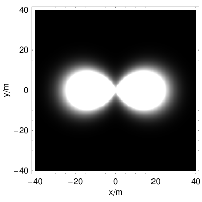
Figure 9: Contour plot: number density of high energy muons in the transverse plane for air showers with primary energy $E_{0}=10^{11}$ GeV and zenith angle $\theta=80^{\circ}$, calculated with the revised Heitler model.

As expected, the number of high energy muons is very limited (Fig. 8). So the detector array will actually record several high energy muons arriving at discrete lateral positions, instead of a continuous density distribution in the transverse plane. Nevertheless, once we have determined the shower core position, our calculated double-lobed distribution (Fig. 9) predicts that the high energy muons arriving at each side of the shower core most probably ($>99\%$) belong to the lobe on the same side, carrying the corresponding charge. The shower core can be located by analyzing the density distribution and energy deposits of plenty lower energy secondary particles [18]. Since we know which side for which type of muon charge from the direction of local geomagnetic field, in this way we can confidently identify these high energy muons with their own charges.

Our final purpose is to obtain the charge ratio $R_{\mu}$ for such high energy muons, which will give us valuable information on the composition of primary cosmic ray particle and the understanding of hadro-production processes. However, we need to point out here that it is impractical to measure the charge ratio on an event-by-event basis. Because of the stochastic nature of extensive air showers, the fluctuation in muon numbers will be large compared to the limited total number of high energy muons in a single event. Also, not all the high energy muons in a particular event will be detected, since the array detectors do not cover the whole region. Therefore, both positive and negative muon numbers should be collected from a large number of inclined EAS events, so that we can get a statistically sound value of $R_{\mu}$ for high energy muons.

6 Summary

In this article we analyzed the possibility of obtaining the charge information of high energy muons in very inclined extensive air showers. We have demonstrated that positive and negative high energy muons in sufficiently inclined air showers can be distinguished from each other through their opposite geomagnetic deviations in the transverse plane. We developed a revised Heitler model to calculate this distinct double-lobed distribution, and studied the condition for the two lobes of either positive or negative muons to be separable with confidence. From our criterion of resolvability, we concluded that a zenith angle $75^{\circ}\leq\theta\leq 85^{\circ}$ will be most suitable for our approach.

There are already some results from full air shower simulations that take into account the geomagnetic effect on muon propagation [12] [19]. They illustrated remarkable double-lobed muon lateral density profile in very inclined air showers, which is in agreement with our expectation qualitatively. However, no present study has fully considered the high energy part of muon content, which can be used to compare with our results. Thus we would like to propose future simulations of very inclined extensive air showers that focus on the behavior of high energy muons. They also have to keep track of the muon charges and the relation to their lateral positions.

For our method to be applicable in measuring the high energy muon charges, there are some requirements on the shower detector performance. First, the muon detectors should be able to measure muon energies up to over $10^{4}-10^{5}$ GeV, so that we can sort out those muons with energies high enough for our purpose. Moreover, since the high energy muons arrive very near the shower core, we would have to look for EAS events whose shower cores are inside the coverage of the detector array. Besides, to distinguish the muons’ charges from their lateral positions, a detector array is expected to have a high resolution in the shower transverse plane.

As far as we are concerned, there are still some technical limitations to the above requirements. For example, the detectors near the shower core are usually saturated with signals from lower energy muons [1]. Therefore, we suggest to employ muon detectors that are especially aimed at detecting high energy muons in the shower array. They should have a high threshold energy up to $10^{4}$ GeV, so as to avoid unwanted signals from low energy muons. Or these detectors may be extensions of existing ones like water Čerenkov detectors, but with special triggers to sort out high energy signals.

Our method not only works for air showers with primary energies over the “ankle” ($\sim 10^{10}$ GeV), it can also be applied to study cosmic rays in the “knee” region. In such cases, the primary energy of the cosmic ray particle is around $10^{6}$ GeV, several orders lower than the examples we studied above. Accordingly, the energies of muons produced by early generation pions range from $10^{2}$ GeV to $10^{3}$ GeV. Produced higher in the atmosphere with lower energies, these muons experience larger lateral deviations, and are more susceptible to the geomagnetic bending. Thus we shall have an even better condition to use our method to obtain the muon charge information. What is more, for such energies below $1000$ GeV, there are alternative ways to distinguish the muon charges [20, 8]. By comparing the results, these experiments can serve as a test to validate or rule out the possible application of our approach.

References

- [1] L. Anchordoqui, M. T. Dova, A. Mariazzi, T. McCauley, T. Paul, S. Reucroft and J. Swain, Annals Phys. 314, 145 (2004) [arXiv:hep-ph/0407020].
- [2] K. Greisen, Phys. Rev. Lett. 16, 748 (1966); G. T. Zatsepin and V. A. Kuzmin, JETP Lett. 4, 78 (1966) [Pisma Zh. Eksp. Teor. Fiz. 4, 114 (1966)].
- [3] D. J. Bird et al., Astrophys. J. 441, 144 (1995); M. Nagano and A. A. Watson, Rev. Mod. Phys. 72, 689 (2000); M. Takeda et al., Astropart. Phys. 19, 447 (2003) [arXiv:astro-ph/0209422].
- [4] For recent reviews, see e.g. T. Stanev, eConf C040802, L020 (2004) [arXiv:astro-ph/0411113]; R. Engel, Nucl. Phys. Proc. Suppl. 151, 437 (2006) [arXiv:astro-ph/0504358].
- [5] E. Zas, New J. Phys. 7, 130 (2005) [arXiv:astro-ph/0504610].
- [6] S. Eidelman et al. [Particle Data Group], Phys. Lett. B 592, 1 (2004).
- [7] R. K. Adair, H. Kasha, R. G. Kellogg, L. B. Leipuner and R. C. Larsen, Phys. Rev. Lett. 39, 112 (1977); W. Y. Hwang and B. Q. Ma, Eur. Phys. J. A 25, 467 (2005) [arXiv:astro-ph/0509118].
- [8] B. Vulpescu et al., Nucl. Instrum. Meth. A 414, 205 (1998); E. B. Beall, FERMILAB-THESIS-2005-74.
- [9] J. Matthews, Astropart. Phys. 22, 387 (2005).
- [10] L. Penchev, P. Doll and H. O. Klages, J. Phys. G 25, 1235 (1999).
- [11] J. Knapp, D. Heck, S. J. Sciutto, M. T. Dova and M. Risse, Astropart. Phys. 19, 77 (2003) [arXiv:astro-ph/0206414].
- [12] M. Ave, R. A. Vazquez and E. Zas, Astropart. Phys. 14, 91 (2000) [arXiv:astro-ph/0011490].
- [13] H. H. Aly, M. F. Kaplon, and M. L. Shen, Nuovo. Cim. 31, 905 (1964).
- [14] J. R. Horandel, J. Phys. G 29, 2439 (2003) [arXiv:astro-ph/0309010].
- [15] C. A. Ayre et al., J. Phys. A 5, L102 (1972).
- [16] T. Hebbeker and C. Timmermans, Astropart. Phys. 18, 107 (2002) [arXiv:hep-ph/0102042].
- [17] S. Ostapchenko, Nucl. Phys. Proc. Suppl. 151, 147 (2006) [arXiv:astro-ph/0412591].
- [18] See, e.g., W. D. Apel et al. [KASCADE Collaboration], arXiv:astro-ph/0510810.
- [19] P. Hansen, T. K. Gaisser, T. Stanev and S. J. Sciutto, Phys. Rev. D 71, 083012 (2005) [arXiv:astro-ph/0411634]; A. Cillis and S. J. Sciutto, arXiv:astro-ph/9908002.
- [20] See, e.g., B. C. Rastin, J. Phys. G 10, 1629 (1984); J. Kremer et al., Phys. Rev. Lett. 83, 4241 (1999).