A simple model for the distribution of quiet Sun magnetic field strengths

Abstract

We derive a first order linear differential equation describing the shape of the probability density function of magnetic field strengths in the quiet Sun (PDF). The modeling is very schematic. It considers convective motions which continuously supply and withdraw magnetic structures. In addition, a magnetic amplification mechanism increases the field strength up to a threshold that cannot be exceeded. These three basic ingredients provide PDFs in good agreement with the PDFs produced by realistic numerical simulations of magneto convection, as well as with quiet Sun PDFs inferred from observations. In particular, the distribution is approximately lognormal, and it produces an excess of magnetic fields (i.e., a hump in the distribution) right before the maximum field strength. The success of this simple model may indicate that only a few basic ingredients shape the quiet Sun PDF. Our approach provides a concise parametric representation of the PDF, as required to develop automatic methods of diagnostics.

1. Introduction

Livingston & Harvey (1975) and Smithson (1975) discovered weak polarization signals in the interior of supergranulation cells. These magnetic signals are known as Inter-Network magnetic fields (IN), Intra-Network fields or, simply, quiet Sun fields. It has been long conjectured that such signals trace a hidden component of the solar magnetic field having most of the unsigned magnetic flux and magnetic energy (e.g., Unno 1959; Stenflo 1982; Yi et al. 1993; Sánchez Almeida 1998, 2004; Schrijver & Title 2003). This suggestion seems to be confirmed by recent measurements (e.g. Stenflo 1982; Faurobert-Scholl 1993; Faurobert-Scholl et al. 1995; Sánchez Almeida & Lites 2000; Socas-Navarro & Sánchez Almeida 2002; Trujillo Bueno et al. 2004; Manso Sainz et al. 2004; Sánchez Almeida 2005), as well as by numerical simulations of magneto convection (e.g. Cattaneo 1999; Emonet & Cattaneo 2001; Stein & Nordlund 2002; Vögler 2003; Vögler et al. 2005). The signals discovered by Livingston & Harvey and Smithson represent the residual left when a magnetic field of complex topology is observed with finite angular resolution (e.g., Emonet & Cattaneo 2001; Sánchez Almeida et al. 2003). Such complex field is to be expected as a result of the MHD interaction between magnetic fields and the random motions associated with the granulation.

Characterizing these IN fields is therefore important, and significant advances have been produced during the last years (see the references given above). Among the observational parameters used for characterization, the probability density function of magnetic field strengths (PDF) turns out to be particularly useful. It is defined as the fraction of quiet Sun occupied by magnetic fields of each strength. It condenses basic physical information like the filling factor, the unsigned flux, and the magnetic energy corresponding to each field strength (see Sánchez Almeida 2004). In addition, some of the diagnostic techniques employ them directly (e.g., Faurobert-Scholl 1993; Faurobert-Scholl et al. 1995; Faurobert et al. 2001; Trujillo Bueno et al. 2004), and PDFs are predicted by the numerical simulations, allowing a direct comparison between simulations and observations (Cattaneo 1999; Stein & Nordlund 2002; Vögler & Schüssler 2003; Vögler et al. 2005). In spite of these advantages, measuring the quiet Sun PDF is not trivial. All direct estimates are strongly biased. The Zeeman signals originate only in regions of significant field strength and net polarity, whereas the Hanle signals are insensitive to the fields stronger than a few hundred G. Domínguez Cerdeña et al. (2006a) carry out a first attempt to provide the full PDF from 0 G to 1800 G. They remove the known biases by using Hanle effect measurements to constrain the shape at weak fields ($<$ 200 G), Zeeman signals for the strong fields (say, $>$ 400 G), and assuming the PDF to be continuous in between. They work out a set of PDFs compatible with the observations and consistent with numerical simulations of magneto-convection. As it is acknowledged by the authors, they carry out an exploratory estimate and therefore further independent work is required for confirmation. Support would be provided if some of the characteristic and unexpected properties of these PDFs can be explained in terms of simple physical mechanisms. In particular, the empirical PDFs show an increase of strong kG fields right before the maximum possible field strength, set by the gas pressure of the quiet photosphere (see the solid line in Fig. 1a with a hump at $B\sim 1700$ G).

Figure 1.— (a) Set of quiet Sun PDFs derived from numerical simulations of magneto convection (the discontinuous lines), and a semi-empirical PDF that fits observed Zeeman and Hanle signals (the solid line). (b) $\kappa$s reproducing the PDFs shown above. The labels in the inset stand for: Vogler $\equiv$ Vögler (2003), and DC et al. $\equiv$ Domínguez Cerdeña et al. (2006a).

Despite the fact that these strong fields occupy only a small fraction of the surface, they contribute with a large part of the quiet Sun unsigned magnetic flux and magnetic energy, which makes them particularly important. Moreover the kG fields turn out to be ideal for studying the quiet Sun magnetism since they show up in unpolarized light images (Sánchez Almeida et al. 2004). The possible physical origin of such a hump is addressed here. We discuss that a terminal hump is to be expected if a magnetic amplification mechanism operates in the quiet Sun. These mechanisms have a long tradition to explain the presence of kG magnetic fields in plage and network regions (Weiss 1966; Parker 1978; Spruit 1979; van Ballegooijen 1984; Sánchez Almeida 2001; Cameron & Galloway 2005). They concentrate weakly magnetized plasma conserving the magnetic flux, which demands increasing the field strength. No matter the details of the mechanism, all of them abruptly die out at the maximum field strength imposed by the gas pressure of the quiet photosphere. The magnetic structures tend to pile up at this limit giving rise to a hump (bottleneck effect). The idea was already put forward by Domínguez Cerdeña et al. (2006b), but it is elaborated in this paper.

We write down a differential equation to describe the time evolution of the IN PDF (§ 2). The stationary solutions of such equation are analyzed in § 3. It is shown how a terminal hump appears in a natural way. The efficiency of the amplification mechanism is parameterized using a coefficient (speed) with units of magnetic field strength per unit time. Given a PDF, one can infer by inversion the speed of the concentration mechanism. The technique is applied to PDFs coming from numerical simulations, as well as to semi-empirical PDFs (§ 4). Other uses and limitations of the model PDFs are discussed in § 5.

2. Differential Equation

We use a heuristic approach to derive an equation for the shape of the PDF $P(B)$. The different mechanisms creating, destroying and modifying magnetic fields determine $P(B)$. Here we consider three of them plus the buffeting of the granulation, namely, (1) a magnetic amplification mechanism that tends to increase the magnetic field strength, (2) the submergence of the existing flux transported by the granulation downdrafts, (3) the emergence of new magnetic flux transported by the granulation upflows, and (4) the buffeting of the granular motions on the magnetic structures. In the stationary state they are perfectly balanced, therefore,

$${{dP(B)}\over{dt}}={{dP_{1}(B)}\over{dt}}+{{dP_{2}(B)}\over{dt}}+{{dP_{3}(B)}\over{dt}}+{{dP_{4}(B)}\over{dt}}=0,$$ (1)

where $dP_{j}/dt$ represents the variation with time produced by the $j$-th mechanism. We proceed by working out the contribution of the four terms separately, and then considering all them together. Simplicity is the main driver therefore a number of simplifying hypotheses restrict the problem to make it tractable.

First, consider the magnetic amplification mechanism. We start off by assuming that the photospheric magnetic fields are made of fluxtubes, each one having a single magnetic field vector and a single cross-section. Four parameters characterize each fluxtube; the magnetic field strength $B_{i}$, the magnetic field inclination $\theta_{i}$, the magnetic field azimuth $\phi_{i}$, and the section $A_{i}$. Then the properties of the photospheric magnetic fields are fully characterized given the four parameters $B_{i},\theta_{i},\phi_{i}$, and $A_{i}$ corresponding to each fluxtube – the subscript $i$ varies from one to the number of fluxtubes present in the photosphere. By definition, and when $\Delta B\rightarrow 0$, $P(B)\,\Delta B$ is the fraction of photospheric volume occupied by all magnetic structures with strengths between $B-\Delta B/2$ and $B+\Delta B/2$. It can be expressed as a sum that considers all fluxtubes,

$$P(B)\,\Delta B={1\over{\sum_{i}\,\upsilon_{i}}}\sum_{i}\,\upsilon_{i}\,\Pi\Big{(}{{B_{i}-B}\over{\Delta B}}\Big{)},$$ (2)

with $\upsilon_{i}$ the volume of the $i-$th fluxtube, and $\Pi$ the rectangle function,

$$\Pi(x)=\cases{1&$|x|<1/2$,\cr 0&elsewhere.}$$ (3)

Given a field strength $B$, the sum in the numerator of equation (2) differs from zero only when $B-\Delta B/2<B_{i}<B+\Delta B/2$ and, therefore, it gives the total volume occupied by fluxtubes with field strengths between $B-\Delta B/2$ and $B+\Delta B/2$. Note also that the normalization constant in the denominator of equation (2) is the volume of the photosphere and, therefore, a constant. In the case of interest, when $\Delta B\rightarrow 0$, the rectangle function can be replaced with a Dirac $\delta$-function since,

$$\delta(x)=\lim_{\Delta x\rightarrow 0}{{\Pi(x/\Delta x)}\over{\Delta x}};$$ (4)

see, e.g., Bracewell (1978). This replacement leads to the compact expression for $P(B)$ adequate for mathematical manipulations,

$$P(B)={1\over{\sum_{i}\,\upsilon_{i}}}\sum_{i}\,\upsilon_{i}\,\delta(B_{i}-B).$$ (5)

Each fluxtube has a single inclination, therefore, we are implicitly assuming that the fluxtubes are straight and longer than the range of heights of the photosphere; see Figure 2. Accordingly, the volume of photosphere occupied by a fluxtube is simply set by its section and inclination,

$$\upsilon_{i}=\Delta z\,A_{i}/\cos\theta_{i},$$ (6)

where $\Delta z$ stands for the vertical extent of the photosphere or, if this is too large for the approximation (6) to hold, $\Delta z$ represents the range of heights to be described by our PDF. We characterize the magnetic amplification mechanism with the rate $\kappa$ at which it changes the magnetic field strength,

$$\kappa(B_{i})={{dB_{i}}\over{dt}}.$$ (7)

The rate has units of magnetic field strength per unit time, and we will call it speed. According to equation (7), the speed only depends on the field strength of the fluxtube. This is a working hypothesis which may not hold in some practical cases, as we point out in § 5. All the magnetic amplification mechanisms proposed so far conserve the magnetic flux so that an increase of field strength comes together with a decrease of the section of the magnetic structure to maintain the product $A_{i}\,B_{i}$ constant,

$${{d}\over{dt}}(B_{i}\,A_{i})=0.$$ (8)

Equations (6) and (8) lead to,

$${{d\upsilon_{i}}\over{dt}}=-{{\upsilon_{i}}\over{B_{i}}}\kappa(B_{i}),$$ (9)

where we assume that the concentration mechanism does not change the field inclination in a preferred sense. Using equations (5) and (9), and the chain rule,

$$\Big{(}-\sum_{i}\,\upsilon_{i}\Big{)}\,{{dP_{1}(B)}\over{dt}}=$$

$$\sum_{i}\,{{\kappa(B_{i})}\over{B_{i}}}\upsilon_{i}\,\delta(B_{i}-B)+\sum_{i}\,\kappa(B_{i})\,\upsilon_{i}\,{{\delta(B_{i}-B)}\over{B_{i}-B}},$$ (10)

where we have employed the expression for the derivative of a $\delta$-function (e.g., Bracewell 1978),

$${{d\delta(x)}\over{dx}}=-\delta(x)/x.$$ (11)

Keeping in mind the following properties,

$${{\kappa(B_{i})}\over{B_{i}}}\delta(B_{i}-B)={{\kappa(B)}\over{B}}\,\delta(B_{i}-B),$$ (12)

and

$$\kappa(B_{i})\,{{\delta(B_{i}-B)}\over{B_{i}-B}}\simeq\Big{[}\kappa(B)+{{d\kappa(B)}\over{dB}}(B_{i}-B)\Big{]}\,{{\delta(B_{i}-B)}\over{B_{i}-B}},$$ (13)

one can rewrite equation (13) as,

$$\kappa(B_{i})\,{{\delta(B_{i}-B)}\over{B_{i}-B}}\simeq\kappa(B)\,{{d\delta(B_{i}-B)}\over{dB}}+{{d\kappa(B)}\over{dB}}\,\delta(B_{i}-B),$$ (14)

and, consequently, equation (10) turns out to yield either,

$$-{{dP_{1}(B)}\over{dt}}\simeq B^{-1}\kappa(B)\,P(B)+\kappa(B){{dP(B)}\over{dB}}+P(B)\,{{d\kappa(B)}\over{dB}},$$ (15)

or, alternatively,

$$-{{dP_{1}(B)}\over{dt}}\simeq{{1}\over{B}}{{d[\kappa(B)\,B\,P(B)]}\over{dB}}.$$ (16)

The previous equation describes the variation with time of the PDF due to a magnetic amplification mechanism with speed $\kappa(B)$. Note that if rather than an amplification mechanism one deals with a magnetic de-amplification mechanism, equation (16) remains valid with $\kappa(B)<0$. Consequently, one can think of $\kappa(B)$ as the average between all the amplification and de-amplification mechanisms operating in the quiet Sun. The existence of de-amplifications is indeed likely since they often come together with the amplification mechanisms (e.g., Spruit 1979; Cameron & Galloway 2005).

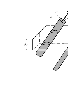
Figure 2.— Schematic with a portion of the photosphere (the box) which includes the full range of photospheric heights $\Delta z$. The two cylinders represent magnetic fluxtubes. The photospheric volume occupied by one of such fluxtubes depends on its cross-section $A$ and its inclination $\theta$, but not on its length if it is longer than $\Delta z/\cos\theta$.

Consider the magnetic fields transported by the downdrafts. In this case magnetic structures disappear in proportion to the existing magnetic structures, i.e.,

$${{dP_{2}(B)}\over{dt}}\simeq-\beta(B)\,P(B),$$ (17)

where $\beta(B)$ provides the rate of submergence per unit time. The rate $\beta(B)$ depends on $B$ to consider that different photospheric field strengths might submerge at different rates.

The emergence of magnetic fields transported by the upflows has the same structure of the submergence but considering a PDF $M(B)$ not necessarily the same as the photospheric PDF. In this case,

$${{dP_{3}(B)}\over{dt}}\simeq\alpha(B)\,M(B),$$ (18)

with the rate of emergence $\alpha(B)$ also depending on the field strength.

The interaction between granular motions and magnetic fluxtubes changes magnetic field inclinations, azimuths, field strengths, and sections. The changes of field strength and section are important, but they have been included in the formalism among the magnetic amplification de-amplification mechanisms. We are left with changes of magnetic field direction, in particular, with changes of magnetic field inclination since the PDF is immune to the azimuths; see equations (5) and (6). We assume, however, that the random granular motions do not change inclinations in a preferred direction which, together with equations (5) and (6), lead to,

$${{dP_{4}(B)}\over{dt}}\simeq 0.$$ (19)

Some limitations of this assumption are pointed out in § 5

Inserting equations (16), (17), (18), and (19) into equation (1), one ends up with the following differential equation for the shape of $P(B)$,

$${{d\big{[}\kappa(B)\,B\,P(B)\big{]}}\over{dB}}\simeq-\beta(B)\,B\,P(B)+\alpha(B)\,B\,M(B).$$ (20)

By definition, the three coefficients that characterize the three physical mechanisms modifying $P(B)$ are all positive, i.e., $\alpha(B)>0$, $\beta(B)>0$ and $\kappa(B)>0$. As we point out above, $\kappa(B)$ stands for the speed of the amplification mechanism whereas $\alpha(B)$ and $\beta(B)$ represent inverse of time scales for the vertical transport of magnetic structures.

From now on we drop from the equations the dependence of all variables on the field strength, which provides manageable expressions without compromising clarity. Then equation (20) becomes,

$${{d(\kappa\,B\,P)}\over{dB}}=-\beta\,B\,P+\alpha\,B\,M.$$ (21)

It is a first order linear differential equation and, consequently, its solutions are given by,

$$P=(B\,\kappa)^{-1}\int_{0}^{B}\alpha\,B^{\prime}\,M\,\exp[-\int_{B^{\prime}}^{B}(\beta/\kappa)\,dB^{\prime\prime}]\,dB^{\prime},$$ (22)

where we have considered that the product $\kappa\,B\,P\rightarrow 0$ when $B\rightarrow 0$. Note that the two coefficients $\alpha$ and $\beta$ cannot be independent since $P$ is a PDF and therefore it must be properly normalized,

$$\int_{0}^{\infty}P\,dB=1.$$ (23)

According to equation (22), $P$ scales with $\alpha$, therefore, given $\kappa$ and $\beta$, a scaling factor applied to $\alpha$ guarantees the proper normalization. It follows from the solution of the differential equation,

$${{d\big{[}\kappa\,B\,f\big{]}}\over{dB}}=-\beta\,B\,f+\alpha_{f}\,B\,M,$$ (24)

which is identical to the original equation (21) except that $\alpha$ has been replaced with an unconstrained $\alpha_{f}$. One can readily show by direct substitution that,

$$P=f/\int_{0}^{\infty}f\,dB,$$ (25)

is a properly normalized solution of equation (21) with,

$$\alpha=\alpha_{f}/\int_{0}^{\infty}f\,dB.$$ (26)

3. Properties of the solutions

3.1. Hump at large field strength

First and most important in the context of this paper, equation (21) predicts PDFs with a hump at large magnetic field strengths. The only condition is an abrupt cease of the magnetic amplification mechanism when $B$ approaches a maximum value $B_{\rm max}$. Explicitly,

$$\kappa\rightarrow 0~{}~{}{\rm when}~{}~{}B\rightarrow B_{\rm max},$$ (27)

with

$$\big{|}{{d\kappa}\over{dB}}\big{|}~{}~{}~{}{\rm large~{}enough}.$$ (28)

Equation (27) puts forward a very natural condition to be satisfied by any amplification mechanism. The magnetic structures must be in mechanical balance within the photosphere and, therefore, the magnetic field strength cannot provide a magnetic pressure exceeding the (gas) pressure of the quiet photosphere (e.g., Spruit 1981). At the base of the photosphere and in the standard 1D model atmospheres (e.g. Maltby et al. 1986),

$$B_{\rm max}\simeq 1800~{}{\rm G}.$$ (29)

In order to prove that conditions (27) and (28) necessarily produce a hump, one rewrites equation (21) as,

$${{dP}\over{dB}}\simeq-\big{[}{{\beta+{{d\kappa}/{dB}}}\over{\kappa}}+B^{-1}\big{]}P,$$ (30)

where we have assumed that the strong fields are produced by the amplification mechanism rather that transported upward by the granular flows ($M\simeq 0$ when $B\rightarrow B_{\rm max}$). Consider the condition (27). It forces

$$P\rightarrow 0~{}~{}{\rm when}~{}~{}B\rightarrow B_{\rm max},$$ (31)

since there are no sources ($M\simeq 0$) and the magnetic fields cannot be intensified to $B=B_{\rm max}$. Because of the limit (31) and the constraint $P>0$,

$${{dP}\over{dB}}<0~{}{\rm when}~{}B\rightarrow B_{\rm max}.$$ (32)

Consequently, the condition for a continuous $P$ to have a maximum ($dP/dB=0$) is equivalent to

$${{dP}\over{dB}}>0,$$ (33)

at a $B<B_{\rm max}$. Using equations (30) and (33), there is a maximum if

$${{d\kappa}\over{dB}}<-\big{[}\beta+{{\kappa}\over{B}}\big{]},$$ (34)

or

$$\big{|}{{d\kappa}\over{dB}}\big{|}>\big{[}\beta+{{\kappa}\over{B}}\big{]}.$$ (35)

These two equations provide specific expressions for what large enough means in equation (28).

3.2. PDF for small magnetic field strengths

We expect the direction of the magnetic field vector to be random when $B\rightarrow 0$. In this case the magnetic forces cannot back-react on the flows and the magnetized plasma is freely dragged, bended and moved around by the granular motions. This continuous buffeting impinges a random tilt to the magnetic fields, which should show no preferred orientation. Domínguez Cerdeña et al. (2006a) argue that this random orientation forces,

$$P\rightarrow 0~{}~{}{\rm when}~{}~{}B\rightarrow 0.$$ (36)

For a point in the atmosphere to have $B=0$, the three Cartesian components of the magnetic field vector must be zero simultaneously, and this is a very improbable event when the orientation of the field is random and therefore the three components independent. Here we go a step further and conjecture that $P$ should follow a Maxwellian distribution, which is the PDF characteristic of the modulus of a vector field with random orientation (see, e.g., Prokhorov 1990; Aguilar Peris 1981). Explicitly,

$$P\simeq{{4}\over{\sqrt{\pi}\,\sigma^{3}}}\,B^{2}\,\exp(-B^{2}/\sigma^{2}),$$ (37)

when $B\rightarrow 0$. In order to obtain this particular shape, $M$ in equation (21) must follow a Rayleigh distribution,

$$M\simeq{2\over{\sigma_{m}^{2}}}\,B\,\exp(-B^{2}/\sigma_{m}^{2}),$$ (38)

with $\sigma=\sigma_{m}\sqrt{5/3}$ and $\alpha=18\kappa/5\sigma\sqrt{\pi}$. This can be checked by direct substitution of $M$ and $P$ into equation (21), considering that $\kappa$ and $\alpha$ do not vary with the magnetic field when $B\rightarrow 0$, and neglecting the influence of the magnetic flux transported downward ($\beta P\ll\alpha M$ when $B\rightarrow 0$).

3.3. Analytical approximation

It was found by Domínguez Cerdeña et al. (2006a) that the PDFs produced by numerical simulations of magneto-convection follow a lognormal distribution, and this shape was adopted to describe $P$ for sub-kG magnetic field strengths. In this case,

$$P={{1}\over{\sqrt{\pi}\,s\,B}}\exp\big{\{}-\big{[}{{\ln(B/B_{s})}\over{s}}\big{]}^{2}\big{\}},$$ (39)

with the parameters $B_{s}$ and $s$ related to the mean and the variance of the distribution. It turns out that equation (21) predicts a lognormal distribution when (a) the influence of $M$ is negligible (e.g., when B is larger than the typical field strengths supplied by the granular upflows), and (b) the various coefficients characterizing the differential equation have a weak dependence on the field strength. Equation (21) can be rewritten as,

$${{d\ln(B\,P)}\over{d\ln B}}=-\big{[}{{\beta}\over{\kappa}}B+{{d\ln\kappa}\over{d\ln B}}\big{]}.$$ (40)

When the variation of the right-hand-side term of this equation with magnetic field is not is not very large, then it can be approximated as,

$${{\beta}\over{\kappa}}B+{{d\ln\kappa}\over{d\ln B}}\simeq a+b\ln B,$$ (41)

with $a$ and $b$ two constants. In this case the integration of equation (40) automatically gives a lognormal (39) with,

$$\ln B_{s}= -a/b,$$ (42)

$$s= \sqrt{2/b}.$$ (43)

Therefore, provided that the approximation (41) is valid, a lognormal yields a good analytical representation of the PDFs proposed in the paper.

3.4. Magnetic flux and magnetic energy

The two terms on the right-hand-side of equation (21) represent the rate of magnetic flux emergence and submergence (§ 2). Since the magnetic amplification mechanisms do not change the flux (§ 2), they have to be equal once integrated over the full range of field strengths. This property is automatically fulfilled by the solutions of equation (21). Integrating (21) from $B=0$ to $B=B_{\rm max}$ and considering the limit (31), then,

$$\int_{0}^{B_{\rm max}}\,\beta\,B\,P\,dB=\int_{0}^{B_{\rm max}}\,\alpha\,B\,MdB,$$ (44)

as demanded by the conservation of magnetic flux. The amplification mechanisms transform weak fields into strong fields. The energy of the distribution scales with the square of the magnetic field strength, therefore, the magnetic amplification mechanism is expected to create magnetic energy. One can show that any amplification mechanism increases the energy coming from below multiplying equation (21) by $B$ an integrating from $B=0$ to $B=B_{\rm max}$. A trivial manipulation leads to,

$$\int_{0}^{B_{\rm max}}\,\beta\,B^{2}\,P\,dB=\int_{0}^{B_{\rm max}}\,\alpha\,B^{2}\,MdB+\int_{0}^{B_{\rm max}}\,\kappa\,B\,PdB.$$ (45)

Keeping in mind that the second term of the right-hand-side is always positive ($\kappa$, $B$ and $P$ are positive), then

$$\int_{0}^{B_{\rm max}}\,\beta\,B^{2}\,P\,dB>\int_{0}^{B_{\rm max}}\,\alpha\,B^{2}\,MdB.$$ (46)

This inequality implies that magnetic energy transported downward (proportional to the left-hand-side term) is always larger than the energy coming from below (the right-hand-side term).

3.5. Examples of PDFs

Figure 3.— (a) PDFs predicted by equation (21) depending on the speed of the amplification mechanism $(\kappa)$. (b) Speeds responsible for the above PDFs. The legend in (a) indicates the only parameter that differs between the reference (the solid line) and the other PDFs.

In order to illustrate some of the properties described above, we integrate equation (21) under simple assumptions that still provide a hump at large field strengths. We consider $\alpha$ and $\beta$ to be constant, whereas $\kappa$ is almost constant up to a magnetic field $B_{\kappa}$ where it abruptly drops to zero in an interval $\Delta B_{\kappa}$, namely,

$$\kappa={{\kappa_{0}}\over{2}}\big{[}1-\tanh\big{(}{{B-B_{\kappa}}\over{\Delta B_{\kappa}}}\big{)}\big{]}.$$ (47)

The symbol $\kappa_{0}$ stands for $\kappa$ when $B\ll B_{k}-\Delta B_{k}$. The differential equation is integrated using a standard fourth-order Runge-Kutta method, from low to strong fields, and using as boundary condition that given in equation (36). The feeding function $M$ is taken to be a Rayleigh distribution as discussed in § 3.2. The solid line in Figure 3a shows $P$ for $B_{\kappa}=1600~{}$G, $\Delta B_{\kappa}=$100 G, $\kappa_{0}/\beta=$500 G and $\sigma_{m}=50$ G, and it is used as a reference to explore the dependence of $P$ on $\kappa$. The curves in Figure 3a have been computed using the speeds shown in Figure 3b. First, note how all PDFs show a terminal hump. The hump rises as the jump of $k$ sharpens (see the dashed line, with $\Delta B_{\kappa}=$25 G), and its position moves according to $B_{\kappa}$ (see the dotted-dashed line, with $B_{\kappa}=$1000 G). The faster the magnetic amplification mechanism the larger the tail of strong fields. The dotted line corresponds to a $\kappa_{0}$ almost twice the reference value. Finally, the tail of strong fields also increases with the magnetic flux supplied by the granulation upflows. The triple dot-dash line is fed with three times more magnetic flux than the reference PDF. This may explain why plage regions have more kG fields than the quiet Sun.

4. Inversion of selected PDFs

Knowing $P$ it is possible to derive by inversion the function $\kappa$ characterizing the concentration mechanism. This is particularly simple for the range of large field strengths, where one expects $M$ to be negligible. Under this condition, equation (21) admits a solution of the kind,

$${{\kappa}\over{\beta}}\,B\,P=\int_{B_{0}}^{B_{\rm max}}\,B^{\prime}\,P\,dB^{\prime}-\int_{B_{0}}^{B}\,B^{\prime}\,P\,dB^{\prime}.$$ (48)

The symbol $B_{0}$ stands for the smallest field strength where $M$ can be neglected ($M\simeq 0$ for $B>B_{0}$). The coefficient $\beta$ has been assumed to be constant for convenience, but this condition can be relaxed if required. Equation (48) provides $\kappa$ given $P$. It has been applied to a set of PDFs to illustrate the feasibility of the inversion. Theses PDFs are shown in Figure 1a, whereas the associated $\kappa$ are in Figure 1b. The solid line corresponds to a semi-empirical PDF that reproduces the level of Zeeman and Hanle signals observed in the quiet Sun (Domínguez Cerdeña et al. 2006a, the reference PDF). Despite all the uncertainties, it represents the kind of the PDF to be expected in the quiet Sun. The inversion provides $\kappa/\beta$, i.e., the speed of the concentration mechanism times the time-scale for the granular downdrafts to remove all magnetic structures from observable layers. In order to reproduce the semi-empirical PDF, $\kappa/\beta$ has to be of the order of 1000 G (between 500 G and 1700 G, according to the solid line in Fig. 1b). In other words, during a time scale $\beta^{-1}$, the concentration mechanism must increase the field strength from zero to 1kG. If we associate $\beta^{-1}$ with the granulation turn-over time, the concentration mechanism must operate with a time-scale of, say, 15 min. This value is not very different from the time-scales characteristic of the concentration mechanisms proposed in the literature. For example, the convective collapse simulations by Takeuchi (1999) create kG fields in minutes, whereas the thermal relaxation proposed by Sánchez Almeida (2001) easily concentrates low magnetic flux structures within a granulation turn-over time. The other PDFs in Figure 1a correspond to numerical simulations of magneto convection by Vögler (2003) having three different levels of unsigned magnetic flux (see the inset). The values of $\kappa/\beta$ are similar to that of the semi-empirical PDF, however, the variation with the field strength is significantly different. They peak at hG field strengths whereas the semi-empirical $\kappa$ has its peak at kG field strengths. The main effect is a reduction of the kG fields of the numerical PDFs with respect to the semi-empirical PDF. As a by product, the gradient of $\kappa$ with $B$ is smaller in the numerical PDF which, according to the discussion in § 3.1, necessarily produces humps that are smaller.

5. Discussion and conclusions

We derive a first order linear differential equation describing the shape of the probability density function of magnetic field strengths in the quiet Sun (PDF). The modeling considers convective motions which continuously supply and remove magnetic structures from the observable layers. In addition, a generic magnetic amplification mechanism tends to increase the field strength up to a maximum threshold. The basic ingredients that we consider yield PDFs in good agreement with the PDFs produced by realistic numerical simulations of magneto convection, as well as with quiet Sun PDFs inferred from observations. In particular, they give a natural explanation for the hump right before the cutoff at 1700 G found by Domínguez Cerdeña et al. (2006b, a). It is produced by the abrupt end of the amplification mechanism at the cutoff. The solutions of our equation provide a parametric family of PDFs as required for diagnostics in automatic inversion procedures (see Socas-Navarro 2001). For example, the PDFs analyzed in § 4 depend on four free parameters which, in principle, can be fitted using four independent observables. We also derive an approximate expression to infer the speed of the amplification mechanism once the PDFs are known. In order to reproduce the semi-empirical PDFs, the amplification mechanism must concentrate field strengths from zero to 1 kG in a time-scale similar to the granulation turn-over time.

The magnetic structure of the quiet photosphere is certainly much more complex than the modeling carried out in the paper, as it is evidenced by the existing numerical simulations of magneto convection (see § 1). To mention just a few potentially important ingredients that we have ignored, the speed of the amplification may depend on the section of the magnetic structure (Spruit 1979), we expect a tendency for the plasma with large field strength to be buoyant and so vertical (e.g. Schüssler 1986), and the fluxtubes forming loops fully embedded in the photosphere do not change their volume under magnetic amplification. This caveat notwithstanding, one should not underestimate the ability of the model to reproduce realistic PDFs. It is a non-trivial property which may reflect that, even if sketchy and primitive, the model contains the basic physical ingredients shaping the PDF of the quiet Sun magnetic fields. Obviously, we cannot discard that the agreement is due to a fortunate coincidence, and so the model is offered here only as a mere possibility to interpret the quiet Sun PDF.

References

- Aguilar Peris (1981) Aguilar Peris, J. 1981, Curso de Termodinámica (Madrid: Alhambra Universidad)
- Bracewell (1978) Bracewell, R. N. 1978, The Fourier Transform and Its Applications (2nd edition) (Tokyo: McGraw Hill)
- Cameron & Galloway (2005) Cameron, R., & Galloway, D. 2005, MNRAS, 358, 1025
- Cattaneo (1999) Cattaneo, F. 1999, ApJ, 515, L39
- Childress & Gilbert (1995) Childress, S., & Gilbert, D. G. 1995, Stretch, Twist, Fold: The Fast Dynamo (Berlin: Springer-Verlag)
- Domínguez Cerdeña et al. (2006a) Domínguez Cerdeña, I., Sánchez Almeida, J., & Kneer, F. 2006a, ApJ, 636, 496
- Domínguez Cerdeña et al. (2006b) —. 2006b, ApJ, 646, 1421
- Emonet & Cattaneo (2001) Emonet, T., & Cattaneo, F. 2001, ApJ, 560, L197
- Faurobert et al. (2001) Faurobert, M., Arnaud, J., Vigneau, J., & Frish, H. 2001, A&A, 378, 627
- Faurobert-Scholl (1993) Faurobert-Scholl, M. 1993, A&A, 268, 765
- Faurobert-Scholl et al. (1995) Faurobert-Scholl, M., Feautrier, N., Machefert, F., Petrovay, K., & Spielfiedel, A. 1995, A&A, 298, 289