Pumping of OH Main-Line Masers in Star-Forming Regions

Abstract

Pumping routes of masers can in principle be recovered from a small matrix of master equations, at an advanced stage of elimination, by tracing back the coefficients to a set of unmodified all-process rate coefficients, drawn from those which appeared in the original set of master equations, prior to any elimination operations. The traceback is achieved by logging the operations carried out on each coefficient. There is no guarantee that a pumping scheme can be represented as a small set of important routes in this way. In the present work, the traceback method is applied to a model which is typical of a large volume of parameter space which produces very strong inversions in the main lines of the rotational ground state of OH, at 1665- and 1667-MHz. For both lines, the pumping scheme is largely restricted to the ${}^{2}\Pi_{3/2}$ stack of rotational levels, and it is possible to list a comparatively small set of routes (less than ten) which provide more than 80 per cent of the inversion. In both cases, the strongest, and simplest, route consists of a radiative upward stage, to the ${}^{2}\Pi_{3/2},J=5/2$ rotational level, followed by a collisional de-excitation to the rotational ground state.

1 Introduction

Sophisticated, many-level, non-local-thermodynamic-equilibrium (NLTE) computations are now routinely used to generate observables, such as the emergent flux and polarization, from maser regions. Such observables are based on NLTE molecular energy-level populations and associated radiation fields, which are the fundamental outputs from the calculations. In general, however, computations of this type yield far less detailed information about the pumping schemes that produce the maser inversions because the NLTE solutions do not explicitly store pumping routes. The combination of radiative transfer and kinetic master equations that comprises a model of a maser environment typically loses track of which pieces of molecular data, from the (typically) thousands that form the input to the computation, are responsible for the resulting inversions.

Our knowledge of maser pumping schemes remains quite patchy. In the case of OH, the pumping scheme for the $1612$-MHz line in long-period variable and supergiant stars is quite well understood (Elitzur, Goldreich & Scoville [1976]; Elitzur [1981]). Absorption of $35$- and $53$-$\mu$m radiation is required to lift population from the ground rotational state to the $J=3/2$ and $J=5/2$ rotational levels of the ${}^{2}\Pi_{1/2}$ stack, followed by a series of radiative decays to the upper state of the $1612$-MHz line. Dickinson [1987] predicted from IRAS data that the two pumping lines should make similar contributions to the pump. A discussion of modern searches for the pumping lines, and an application of the technique used in the present work (to an OH/IR star envelope that is far from typical) appears in Gray, Howe & Lewis [2005]. Investigations into the pumping of the OH ground-state main lines in stellar envelopes have also been carried out (Collison & Nedoluha [1993],[1994]).

A much less complete picture emerges for OH in star-forming regions, particularly for the ground-state main lines at $1665$ and $1667$ MHz. One ingredient that is widely believed to be important in the pumping of these lines is far-infrared (FIR) line overlap (Litvak [1969]; Lucas [1980]; Bujarrabal et al. [1980]). Detailed models produced after corrected collisional data became available (Dixon, Field & Zare [1985]; Andresen, Hausler & Lülf [1984]) have added further insights. Piehler & Kegel [1989] reject a photodissociative pump, whilst Kylafis & Norman [1990] reject a predominantly collisional scheme. Detailed many-level models, for example, Cesaroni & Walmsley [1991], Gray, Doel & Field [1991], and Pavlakis & Kylafis [1996] suggest a combination of FIR line overlap and an FIR continuum radiation field are significant components of the pump, but the details remain obscure. Recent work on the pumping of $1667$-MHz masers in megamaser sources [2005] links the inversion with FIR radiation at $60$ $\mu$m.

An alternative approach to the analysis of pumping schemes is required: one which reveals significantly more detail than broad inferences from NLTE computations. One such alternative was outlined by Sobolev [1986] and references thererin. This method involves treating the population flow as a set of cycles, with varying numbers of links. These cycles were later compared by analogy with electronic circuits governed by Kirchoff’s Laws [1994a]. Some subset of these cycles will be important for sustaining each maser inversion. Finding the strongest component of the pump was introduced as an analytic optimisation problem, but the suggestion that was followed is that the whole method be developed as a Monte-Carlo computer code, providing mainly statistical information about pumping schemes. This program was used to analyse the pumping scheme for water masers [1989], where it was estimated that a very large number of cycles would need to be traced in order to obtain $75$ per cent of the population flow. The most sophisticated use of this Monte-Carlo scheme is the analysis of pumping routes in methanol masers [1994a, 1994b]. This work was successful in identifying ‘bottleneck’ transitions, following modifications due to saturation, and in computing the percentage of the maser flux produced as a function of the number of links in a cycle. A significant proportion of the flux depended on complicated cycles involving at least $25$ links [1994a].

The method I use to analyse pumping routes in the present work is related to the flow cycles discussed above [1994a], but here the relationship between simple analytic expressions for the inversion, and rate coefficients, from a partially eliminated matrix of master equations, is made explicit. The method also draws heavily on the simple interpretation of the decomposition of a rate coefficient, after an arbitrary number of matrix eliminations, into two sub-expressions. One of these is the same coefficient at an earlier stage of elimination, and the other is a route via a level equal to the row and column just eliminated. Further details of the method are explained in Gray, Howe & Lewis, [2005]. A summary is given in Section 2 below.

2 A summary of the traceback method

I begin with some definitions. The symbol $k_{x,y}^{p}$ is an all-process rate coefficient, representing the flow of population from energy level $x$ to energy level $y$ in a system of master equations which is at elimination stage $p$. For historical reasons, the elimination stage is defined to be $p=n+1$ where $n$ is the number of rows (or columns) remaining in the matrix. As elimination proceeds, $n$ decreases, and has the value $3$ when the matrix has been reduced to $2\times 2$ form. I define the original matrix to be the matrix formed from the set of master equations prior to any elimination operations being carried out; it is a square matrix of size $N\times N$, where $N$ is the number of energy levels in the molecular model. If $x=y$, the coefficient is diagonal, and takes on the meaning of the sum of all rate coefficients out of level $x$. It can be proved by induction (see Appendix A) that, provided this definition of a diagonal coefficient holds at $p=N+1$, it holds for all smaller values of $n$ until matrix elimination reaches a $2\times 2$ form. Where it is necessary to raise a coefficient to a power, it is always enclosed in brackets with the elimination stage inside, and the power outside the brackets.

The coupled radiative transfer and kinetic master equations are solved by a standard numerical method [1994]. The same equations are then re-solved by a naive matrix elimination technique, in which an all-process rate coefficient, at elimination stage $p-1$, can be written as

$$k_{i,j}^{p-1}=k_{i,j}^{p}\pm k_{i,p-1}^{p}k_{p-1,j}^{p}/k_{p-1,p-1}^{p}$$ (1)

where the $-$sign applies only to modification of diagonal coefficients, and where the denominator in the second term on the right-hand side, a diagonal coefficient, acts as a normalising factor, and this whole term represents the introduction of a new link to the coefficient, transfering population from level $i$ to level $j$ via level $p-1$.

Operations of the type shown in eq.(1) are logged and divided into three types, depending on the relative sizes of the two terms on the right-hand side. If the first term is larger than the second by a factor of at least $1/\epsilon$, where $\epsilon$ is a parameter less than $1$, the operation is flagged as ‘unmodified’. This instructs the tracer code, introduced in Gray et al. [2005], to treat $k_{i,j}^{p-1}$ as unchanged from its previous value. If the first term is smaller than the second by a factor smaller than $\epsilon$, the operation is flagged as ‘replacement’: in this case the $k_{i,j}^{p}$ is discarded in favour of the new route via level $p-1$. The third option (an ‘amendment’) requires that both parts of the expression be kept.

The computer code tracer takes coefficients from a matrix reduced to a state where $p$ is small (typically $4$ or $5$), and expands it back to forms with higher $p$, using the information contained in the operation log to simplify the expressions as far as possible. Values for inversions calculated by the standard numerical method are compared with those computed from coefficients returned by tracer as a check that $\epsilon$ has been made small enough (or conversely that sufficient information has been retained).

Providing that the pumping scheme is sufficiently simple (and there is no guarantee of this) it is possible to use tracer in several stages to expand coefficients at elimination stage $p\sim 4$ back to the original coefficients of the unmodified matrix, that is where $p=N+1$. Once this has been achieved, the coefficient $k_{i,j}^{p}$, for small $p$, has been represented in terms of original all-process rate coefficients that can be expressed directly in terms of the molecular parameters supplied to the model (Einstein A-values and collisional rate coefficients) and the radiation energy density, or mean intensity.

2.1 inversions

Expansion of a single coefficient does not, of course, reveal the pumping scheme. In order to do this, we need to recover the net effect of a set of coefficients which together yield an inversion in the transition of interest. The method used is simply to find an analytic expression for the required inversion in terms of coefficients at small $p$ and then use tracer on all antagonistic pairs of coefficients which represent forward (pumping) and reverse (anti-pumping) routes. It is important to note that some terms, which are large in the tracer expansion of an individual coefficient, may contribute almost nothing to an inversion because they are paired with a term of the same magnitude in the expansion of the reverse coefficient. I give below the analytic formulae for the inversions in the main-line ground state maser transitions of OH. The formula for $1665$ MHz (level $3$ to level $1$) is given in terms of coefficients with $p=4$, whilst the analogous formula for $1667$ MHz is written with $p=5$. For a listing of level numbers in terms of the more usual quantum-mechanical designations for OH, see Table 1. The level numbers used in the present work are ordered upwards by energy, with level $1$ being the ground state.

$$\Delta\rho_{3,1}=\frac{{\cal N}k_{2,2}^{4}}{3D}\left\{\!k_{1,3}^{4}-k_{3,1}^{4}+\!\left(\frac{k_{1,2}^{4}k_{2,3}^{4}-k_{3,2}^{4}k_{2,1}^{4}}{k_{2,2}^{4}}\!\right)\!\right\}$$ (2)

$$\Delta\rho_{4,2} \!\!\!\!\!=\!\!\!\!\! \frac{{\cal N}X}{5Dk_{4,4}^{5}}\left\{\!k_{2,4}^{5}-k_{4,2}^{5}+\frac{k_{1,1}^{5}}{X}(k_{2,3}^{5}k_{3,4}^{5}-k_{4,3}^{5}k_{3,2}^{5})\right.$$ (3)

$$\!\!\!\!\!+\!\!\!\!\! \frac{k_{3,3}^{5}}{X}(k_{2,1}^{5}k_{1,4}^{5}-k_{4,1}^{5}k_{1,2}^{5})\!+\!\frac{k_{2,1}^{5}k_{1,3}^{5}k_{3,4}^{5}-k_{4,3}^{5}k_{3,1}^{5}k_{1,2}^{5}}{X}$$

$$\!\!\!\!\!+\!\!\!\!\! \left.\frac{k_{2,3}^{5}k_{3,1}^{5}k_{1,4}^{5}-k_{4,1}^{5}k_{1,3}^{5}k_{3,2}^{5}}{X}\!\right\}$$

where $X=k_{1,1}^{5}k_{3,3}^{5}-k_{1,3}^{5}k_{3,1}^{5}$ and $\cal N$ is the total number density of OH used in the model.

Equations 2 and 3 have a number of important features: both have, multiplying the outer bracket, a positive definite term which modifies the overall magnitude of the inversion, but which does not decide its sign. It is obvious that $X$ is positive definite because the diagonal term $k_{1,1}^{5}$ must contain $k_{1,3}^{5}$ as part of its sum, and similarly $k_{3,3}^{5}$ contains $k_{3,1}^{5}$. The negative part of the expression, as written above, is therefore cancelled exactly. The denominator $D$ is shown to be positive definite in Appendix B. Both inversions are quoted per magnetic sublevel, giving rise to the $3$ in the denominator of eq.(2) amd the $5$, in eq.(3). Inside the outer bracket, groups of coefficients are written in antagonistic pairs, which represent the flow of population between the pair of levels that form the transition of interest. The pair of coefficients involving only the upper and lower levels of the transition of interest will be referred to as forming the ‘direct’ route (even though, on expansion, many other levels will in general be involved). Other pairs, which involve one or two other un-eliminated levels, will be referred to as forming ‘indirect’ routes, because they involve levels other than those that make up the transition in question before any expansion has been performed with tracer. The reason for the greater complexity of eq.(3) is that it is evaluated for $p=5$ (a $4\times 4$ matrix) whilst eq.(2) uses $p=4$.

Table 1: Quantum-mechanical designations of the first twenty hyperfine levels of OH in Hund’s case (a) notation.

Level Number	Designation
1	${}^{2}\Pi_{3/2},J=3/2,(1-)$
2	${}^{2}\Pi_{3/2},J=3/2,(2-)$
3	${}^{2}\Pi_{3/2},J=3/2,(1+)$
4	${}^{2}\Pi_{3/2},J=3/2,(2+)$
5	${}^{2}\Pi_{3/2},J=5/2,(2+)$
6	${}^{2}\Pi_{3/2},J=5/2,(3+)$
7	${}^{2}\Pi_{3/2},J=5/2,(2-)$
8	${}^{2}\Pi_{3/2},J=5/2,(3-)$
9	${}^{2}\Pi_{1/2},J=1/2,(0+)$
10	${}^{2}\Pi_{1/2},J=1/2,(1+)$
11	${}^{2}\Pi_{1/2},J=1/2,(0-)$
12	${}^{2}\Pi_{1/2},J=1/2,(1-)$
13	${}^{2}\Pi_{1/2},J=3/2,(1-)$
14	${}^{2}\Pi_{1/2},J=3/2,(2-)$
15	${}^{2}\Pi_{1/2},J=3/2,(1+)$
16	${}^{2}\Pi_{1/2},J=3/2,(2+)$
17	${}^{2}\Pi_{3/2},J=7/2,(4-)$
18	${}^{2}\Pi_{3/2},J=7/2,(3-)$
19	${}^{2}\Pi_{3/2},J=7/2,(4+)$
20	${}^{2}\Pi_{3/2},J=7/2,(3+)$

3 The OH Pumping Model

The pump-route traces for both main lines were drawn from the same model. This was a single computation chosen from a large parameter-space search using a slab-geometry accelerated lambda iteration (ALI) code [1985]. This code incorporates far-infrared (FIR) line overlap (Jones et al. [1994]; Stift [1992]). It has previously been applied in the study of several OH and H₂O maser environments [2005, 2001, 1997, 1995].

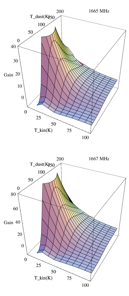
Figure 1: Integrated gains in the $1665$ (top) and $1667$-MHz lines for a dataset, which includes the chosen ALI model, plotted against the kinetic and dust temperatures. Physical conditions not shown on the axes are those from Table 2. Saturation of the maser transitions is not included.

The only criterion for selection was that the chosen computation came from near the peak of the parameter-space search for unsaturated integrated gain in both the ground-state main lines. Fig. 1 shows unsaturated integrated gain plotted as a function of kinetic and dust temperatures for part of the parameter space search, including the model chosen. Parameters of the selected model itself are shown in Table 2. Unsaturated integrated gains predicted for the selected model were $20.039$ at $1665$ MHz and $35.661$ at $1667$ MHz. Saturation would limit any real maser to values in the range $10$-$14$ as the overall amplification factor is the exponential of the integrated gain through the model. Competitive gain in saturation [1988], is effective at converting initial inversion at $1667$ MHz to maser amplification at $1665$ MHz, so the model is probably consistent with observations in Galactic star-forming regions which show that $1665$ MHz is usually the dominant main-line, and ground-state, OH maser (for example, Gaume & Mutel [1987]). An additional inversion was present in the ground state at $1720$ MHz, but the only significant excited-state inversions in this model were the ${}^{2}\Pi_{3/2},J=5/2$ main lines at $6035$ and $6030$ MHz.

Table 2: Main parameters of the ALI model

Parameter	Value
Total depth	$3.0\times 10^{13}$ m
Depth of chosen slab	$2.0\times 10^{13}$ m
Thickness of chosen slab	$4.7\times 10^{12}$ m
H2 number density	$1.0\times 10^{7}$ cm-3
Fractional abundance of OH	$2.0\times 10^{-7}$
Kinetic temperature	$30$ K
Dust temperature	$70$ K
Bulk velocity shift	$0.0$ km s-1
Microturbulence	$0.0$ km s-1

The tracer method can only work under one set of conditions at once, including the radiation field. Therefore, the naive matrix elimination method was run on a single selected slab drawn from the total of $85$ in the model. These are arranged logarithmically, such that the depth of slab $k$ is given by

$$z_{k}=z_{1}(z_{M}/z_{1})^{k/M}$$ (4)

where $z_{k}$ is the depth of layer $k$, and there are $M$ layers altogether. The selected slab was $k=80$; this slab was chosen to have the peak inversion found anywhere in the model at $1665$ MHz. It also turns out that the maximum $1667$-MHz inversion was also found in the same slab. The absolute inversions in the two lines for the chosen slab are $\Delta\rho_{3,1}=7.311\times 10^{-3}$ cm^-3 and $\Delta\rho_{4,2}=8.683\times 10^{-3}$ cm^-3. The overall number density of OH, from Table 2, is $2.0$ cm^-3. The tracer analysis which follows, if it is to have any generality, therefore includes the assumptions that the pumping schemes in other slabs are generally similar to those analysed here, and that neighbouring models, such as those forming the grids in Fig. 1, also have pumping schemes broadly similar to that of the chosen model and slab. This assumption is probably reasonable, given that the model slab is uniform, and that the integrated gains in Fig. 1 vary smoothly in the vicinity of the chosen model.

3.1 molecular data

The molecular data supplied as input to the ALI code comprised energies of the $48$ hyperfine levels used and Einstein A-values for the radiatively allowed transitions [1977], complemented by collisional rate coefficients from Offer, van Hemmert & van Dishoeck [1994]. This set of coefficients allows for collisions of OH with both ortho- and para-hydrogen. Molecular hydrogen was assumed to be distributed between the ortho- and para- species at a ratio of $3$ to $1$.

4 The 1665 MHz Pump

As the highest level involved in the $1665$-MHz transition is level $3$, it is convenient to begin from a $3\times 3$ matrix, which yields the inversion in eq.(2). For this transition, eq.(2) has two antagonistic groups of rate coefficients which control the inversion: the first is the ‘direct’ route, $k_{1,3}^{4}-k_{3,1}^{4}$ and the second, the ‘indirect’ route via level $2$, $(k_{1,2}^{4}k_{2,3}^{4}-k_{3,2}^{4}k_{2,1}^{4})/k_{2,2}^{4}$. On examining the magnitudes of these two expressions, the direct route was found to have the value $1.05\times 10^{-4}$ s^-1, and the indirect route, $9.07\times 10^{-5}$ s^-1. Both terms are positive, and therefore inverting, and similar in magnitude, so they provide roughly comparable contributions to the overall pump. It is therefore clear that both routes must be taken into account when tracing back towards earlier elimination stages. Fortunately, the trace remains resonably simple, with two components of the direct route supplying $83$% of it, and three components of the indirect route contributing $80.5$% of the total in that system. This total of five dominant terms, which together provide 81.8 per cent of the $1665$ MHz inversion, are discussed below in detail.

4.1 Route 1

Route 1 is the strongest term in the expansion of the direct pump, $k_{1,3}^{4}-k_{3,1}^{4}$. It has a rate of $6.01\times 10^{-5}$ s^-1 (relative strength $1.0$) and the expression in rate-coefficients at elimination stage $6$ is $(k_{1,5}^{6}k_{5,3}^{6}-k_{3,5}^{6}k_{5,1}^{6})/k_{5,5}^{6}$. Route 1 is the strongest of the five dominant routes, and also the simplest, because further expansion of the coefficients in the numerator with tracer produces little additional complexity. Writing unmodified coefficients (at elimination stage $N+1$) without superscript, I found $k_{1,5}^{6}=k_{1,5}$ and similarly for $k_{5,1}^{6}$. The expansion of $k_{5,3}^{6}$ and $k_{3,5}^{6}$ produced original coefficients, and extra terms (via a list of ‘amendment’ operations). However, all but one of these were found to be weak and anti-inverting. The remaining route was a weakly inverting pump via level $15$. However, it was negligible compared to the route using the original coefficients, and to Route 3 (see below). Denoting Route 1 by $R1$, the pump route can therefore be expressed as

$$R1=(k_{1,5}k_{5,3}-k_{3,5}k_{5,1})/k_{5,5}^{6}$$ (5)

Note that the denominator in eq.(5) is left evaluated at elimination stage $6$ for simplicity. As a sum of rate-coefficients, it is positive definite and cannot control the sign of the expression. Important original, or unmodified, all-process rate-coefficients appear in Table 3. Route 1 is also displayed by the black arrows in Figure 2.

4.2 Route 2

Route 2 is the strongest term in the expansion of the indirect pump. It has the expression,

$$R2=(k_{1,5}^{6}k_{5,2}^{6}k_{2,4}^{6}k_{4,3}^{6}-k_{3,4}^{6}k_{4,2}^{6}k_{2,5}^{6}k_{5,1}^{6})/(k_{2,2}^{4}k_{4,4}^{5}k_{5,5}^{6})$$ (6)

and a rate equal to $4.86\times 10^{-5}$ s^-1. It has a relative strength (compared to Route 1) of $0.808$. Unlike Route 1, the expansion of Route 2 with tracer introduces a complicated web of routes, not all of which have been traced fully. Three terms control $73$ per cent of Route 2. When fully expanded back to unmodified coefficients, these three components of Route 2 are

$$R2 \!\!\!\!\!\!=\!\!\!\!\!\! \frac{k_{1,5}k_{5,2}k_{2,6}k_{6,4}k_{4,7}k_{7,3}-k_{3,7}k_{7,4}k_{4,6}k_{6,2}k_{2,5}k_{5,1}}{k_{2,2}^{4}k_{4,4}^{5}k_{5,5}^{6}k_{6,6}^{5}k_{7,7}^{8}}$$ (7)

$$\!\!\!\!\!\!+\!\!\!\!\!\! \frac{k_{1,5}k_{5,2}k_{2,6}k_{6,4}k_{4,8}k_{8,20}k_{20,7}k_{7,3}-\Omega_{2B}}{k_{2,2}^{4}k_{4,4}^{5}k_{5,5}^{6}k_{6,6}^{5}k_{7,7}^{8}k_{8,8}^{9}k_{20,20}^{21}}$$

$$\!\!\!\!\!\!+\!\!\!\!\!\! \frac{k_{1,5}k_{5,2}k_{2,10}k_{10,14}k_{14,4}k_{4,7}k_{7,3}-\Omega_{2C}}{k_{2,2}^{4}k_{4,4}^{5}k_{5,5}^{6}k_{10,10}^{5}k_{14,14}^{15}k_{7,7}^{8}}$$

where $\Omega_{2B}$ and $\Omega_{2C}$ are reverse routes, formed from a product of rate coefficients with each pair of levels reversed with respect to those of the forward route; $\Omega_{2A}$ is written out in full. The lines of eq.(7) correspond to the A, B and C subroutes in Fig. 2. The loss of $27$ per cent of Route 2, missing from eq.(7), arises from ignoring $k_{5,6}^{7}k_{6,2}/k_{6,6}^{7}$ in favour of $k_{5,2}$ in the expansion of $k_{5,2}^{6}$ (and a similar approximation in the reverse route). This omission is comparable, in magnitude, to ignoring the fourth and fifth dominant terms (the remaining two from the indirect pump). The second and third lines in eq.(7) are of comparable strength, and these are both about 1/5 of the strength of the route on the first line. The web of transitions comprising Route 2 is represented by blue arrows in Fig. 2 (except for transitions already marked as part of Route 1).

4.3 Route 3

Route 3 comes from the direct part of the pump, and has a rate of $2.72\times 10^{-5}$ s^-1 (relative strength $0.453$), placing it third in strength of the five dominant terms. The expression for $R3$ is

$$(k_{1,4}^{5}k_{4,3}^{5}-k_{3,4}^{5}k_{4,1}^{5})/k_{4,4}^{5}$$ (8)

The expansion of Route 3 leads to a complex web of routes most of which, for brevity, have been omitted here. The strongest three routes, when fully traced back to unmodified coefficients, appear in eq.(9). These three together account for only $50$ per cent of Route 3. Six terms appear in eq.(9) because some of the expansion involves amendment operations which add terms. The first four terms correspond to Route 3A, and the last pair are Route 3B and Route 3C, respectively. Reverse routes are written in full except for in the third line.

$$R3 \!\!\!\!\!\!=\!\!\!\!\!\! \frac{k_{1,9}k_{9,4}k_{4,7}k_{7,3}-k_{3,7}k_{7,4}k_{4,9}k_{9,1}}{k_{4,4}^{5}k_{7,7}^{8}k_{9,9}^{10}}$$ (9)

$$\!\!\!\!\!\!+\!\!\!\!\!\! \frac{k_{1,9}k_{9,4}k_{4,8}k_{8,20}k_{20,7}k_{7,3}-k_{3,7}k_{7,20}k_{20,8}k_{8,4}k_{4,9}k_{9,1}}{k_{4,4}^{5}k_{7,7}^{8}k_{8,8}^{9}k_{9,9}^{10}k_{20,20}^{21}}$$

$$\!\!\!\!\!\!+\!\!\!\!\!\! \frac{k_{1,9}k_{9,13}k_{13,10}k_{10,14}k_{14,4}k_{4,7}k_{7,3}-\Omega_{3Aiii}}{k_{4,4}^{5}k_{7,7}^{8}k_{9,9}^{10}k_{10,10}^{11}k_{13,13}^{14}k_{14,14}^{15}}$$

$$\!\!\!\!\!\!+\!\!\!\!\!\! \frac{k_{1,9}k_{9,13}k_{13,4}k_{4,7}k_{7,3}-k_{3,7}k_{7,4}k_{4,13}k_{13,9}k_{9,1}}{k_{4,4}^{5}k_{7,7}^{8}k_{9,9}^{10}k_{13,13}^{14}}$$

$$\!\!\!\!\!\!+\!\!\!\!\!\! \frac{k_{1,10}k_{10,14}k_{14,4}k_{4,7}k_{7,3}-k_{3,7}k_{7,4}k_{4,14}k_{14,10}k_{10,1}}{k_{4,4}^{5}k_{7,7}^{8}k_{10,10}^{11}k_{14,14}^{15}}$$

$$\!\!\!\!\!\!+\!\!\!\!\!\! \frac{k_{1,5}k_{5,4}k_{4,3}-k_{3,4}k_{4,5}k_{5,1}}{k_{4,4}^{5}k_{5,5}^{6}}$$

4.4 Route 4

Route 4 comes from the indirect part of the pump; it has a rate equal to

$$R4=(k_{1,5}k_{5,2}k_{2,6}k_{6,3}^{7}-k_{3,6}^{7}k_{6,2}k_{2,5}k_{5,1})/(k_{2,2}^{4}k_{5,5}^{6}k_{6,6}^{7})$$ (10)

with a numerical value of $1.31\times 10^{-5}$ s^-1 (relative strength = $0.218$).

4.5 Route 5

Route 5 is also part of the indirect pump; it has a rate equal to

$$R5=\frac{k_{1,5}k_{5,2}k_{2,10}k_{10,3}^{11}-k_{3,10}^{11}k_{10,2}k_{2,5}k_{5,1}}{k_{2,2}^{4}k_{5,5}^{6}k_{10,10}^{11}}$$ (11)

with a numerical value of $1.13\times 10^{-5}$ s^-1 (relative strength = $0.188$).

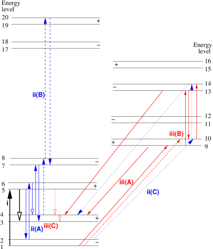
Figure 2: Principal pumping routes for the $1665$ MHz maser under the conditions of Table 2. Energy levels are numbered following the scheme in Table 1, and are marked with a parity assignment (+ or -). Energy gaps between levels are not drawn to scale. Route 1 transitions are shown in black; additional transitions appearing in Route 2 are drawn in blue, and further additions from Route 3 are in red. Transitions appearing from an ‘A’ sub-route have solid lines, those from a ‘B’ sub-route are marked by dashed lines, those from a ‘C’ subroute, by dotted lines. For simplicity, only the forward (pumping) routes are shown for each antagonistic pair, and transitions appearing in more than one route are drawn only once. A solid arrowhead indicates a transition allowed for electric dipole radiation; a hollow arrowhead indicates a radiatively forbidden transition in which population transfer can be considered to proceed via collisions only.

4.6 Summary

The $1665$ MHz pump, though complex, is simple enough to allow a large percentage of its strength to be represented in a modest number of terms. The overall degree of complexity is similar to that found for the $1612$ MHz line in the OH/IR stellar envelopes studies in Gray, Howe & Lewis [2005]. In contrast to that case, in which transfer to the ${}^{2}\Pi_{1/2}$ stack from the ground state by $53$ $\mu$m radiation is amongst the most important processes, the $1665$ MHz pump tends to stay largely within the ${}^{2}\Pi_{3/2}$ stack, with transfer to ${}^{2}\Pi_{1/2}$ appearing only in weaker terms of Route 2, and in Route 3. The strongest pump route of all, Route 1, is extremely simple, comprising only two parts: a radiative FIR absorption from the ground state up to ${}^{2}\Pi_{3/2},J=5/2$, and a collisional decay back to level $3$ in the upper part of the ground-state lambda doublet. This downward leg must be collisional because the upper part of the ground-state lambda doublet and the lower part of the excited-state lambda doublet have the same parity, making this transition radiatively forbidden.

Most of the transitions shown in Fig. 2 are radiative, but there are a significant number of important links which must be predominantly collisional, either because the transitions involved are within lambda doublets and have a very small A-value, or they are radiatively forbidden by parity or other quantum-mechanical selection rules. No part of the pumping scheme involves levels higher than those in the ${}^{2}\Pi_{3/2},J=7/2$ lambda doublet.

5 The 1667 MHz Pump

This pumping scheme was traced from a $4\times 4$ matrix, with the inversion given by eq.(3). The inversion expression is therefore considerably more complicated than in the case of $1665$ MHz, but the compensation for this is reduced complexity in the traceback. Seven contributions to the inversion were found which had an inverting effect of at least ten per cent of the strongest. Of these seven routes, the strongest pair account for $56.5$ per cent of the total inversion. In fully traced-back form, the seven routes become:

$$R1=\frac{k_{2,6}k_{6,4}-k_{4,6}k_{6,2}}{k_{6,6}^{7}}$$ (12)

where $R1$ is taken to have a relative strength of $1.0$, and

$$R2 \!\!\!\!\!=\!\!\!\!\! \frac{k_{2,5}k_{5,1}k_{1,5}k_{5,3}k_{3,7}k_{7,4}-k_{4,7}k_{7,3}k_{3,5}k_{5,1}k_{1,5}k_{5,2}}{[k_{5,5}^{6}]^{2}k_{7,7}^{8}X}$$ (13)

$$\!\!\!\!\!+\!\!\!\!\! \frac{k_{2,5}k_{5,1}k_{1,5}k_{5,3}k_{3,7}k_{7,20}k_{20,8}k_{8,4}-\Omega_{R2}}{[k_{5,5}^{6}]^{2}k_{7,7}^{8}k_{8,8}^{9}k_{20,20}^{21}X}=0.413R1$$

$$R3=\frac{k_{2,10}k_{10,14}k_{14,4}-k_{4,14}k_{14,10}k_{10,2}}{k_{10,10}^{11}k_{14,14}^{15}}=0.290R1$$ (14)

$$R4 \!\!\!\!\!=\!\!\!\!\! \frac{k_{1,1}^{5}(k_{2,6}k_{6,3}k_{3,7}k_{7,4}-k_{4,7}k_{7,3}k_{3,6}k_{6,2})}{k_{7,7}^{8}k_{8,8}^{9}X}$$ (15)

$$\!\!\!\!\!+\!\!\!\!\! \frac{k_{1,1}^{5}(k_{2,6}k_{6,3}k_{3,7}k_{7,20}k_{20,8}k_{8,4}-\Omega_{R4})}{k_{7,7}^{8}[k_{8,8}^{9}]^{2}k_{20,20}^{21}X}=0.255R1$$

$$R5 \!\!\!\!\!=\!\!\!\!\! \frac{k_{1,1}^{5}(k_{2,10}k_{10,3}k_{3,7}k_{7,4}-k_{4,7}k_{7,3}k_{3,10}k_{10,2})}{k_{7,7}^{8}k_{10,10}^{11}X}$$ (16)

$$\!\!\!\!\!+\!\!\!\!\! \frac{k_{1,1}^{5}(k_{2,10}k_{10,14}k_{14,3}k_{3,7}k_{7,4}-\Omega_{R5})}{k_{7,7}^{8}k_{10,10}^{11}k_{14,14}^{15}X}=0.228R1$$

$$R6=\frac{k_{3,3}^{5}(k_{2,5}k_{5,1}k_{1,5}k_{5,4}\!-\!k_{4,5}k_{5,1}k_{1,5}k_{5,2})}{[k_{5,5}^{6}]^{2}X}=0.203R1$$ (17)

$$R7 \!\!\!\!\!=\!\!\!\!\! \frac{k_{3,3}^{5}(k_{2,5}k_{5,1}k_{1,9}k_{9,4}-k_{4,9}k_{9,1}k_{1,5}k_{5,2})}{k_{5,5}^{6}k_{9,9}^{10}X}$$ (18)

$$\!\!\!\!\!+\!\!\!\!\! \frac{k_{3,3}^{5}(k_{2,5}k_{5,1}k_{1,9}k_{9,13}k_{13,10}k_{10,14}k_{14,4}-\Omega_{R7B})}{k_{5,5}^{6}k_{9,9}^{10}k_{10,10}^{11}k_{13,13}^{14}k_{14,14}^{15}X}$$

$$\!\!\!\!\!+\!\!\!\!\! \frac{k_{3,3}^{5}(k_{2,5}k_{5,1}k_{1,9}k_{9,13}k_{13,4}-\Omega_{R7C})}{k_{5,5}^{6}k_{9,9}^{10}k_{13,13}^{14}X}=0.112R1$$

where some reverse routes have been compressed to the $\Omega$-notation, as for $1665$ MHz. For the equations in the set eq.(13) - eq.(15) where there is more than one line, the lines are ordered by inverting strength. The first line is termed the ‘A’ route, then the ‘B’ route. Only Route 7 has a ‘C’ route. In all these equations, inverting strengths have been given relative to the expression in eq.(12). The absolute value of this expression for $R1$ is $6.89\times 10^{-5}$ s^-1. The seven routes represented by eq.(12) - eq.(15) are shown on a schematic energy-level diagram of OH in Fig. 3

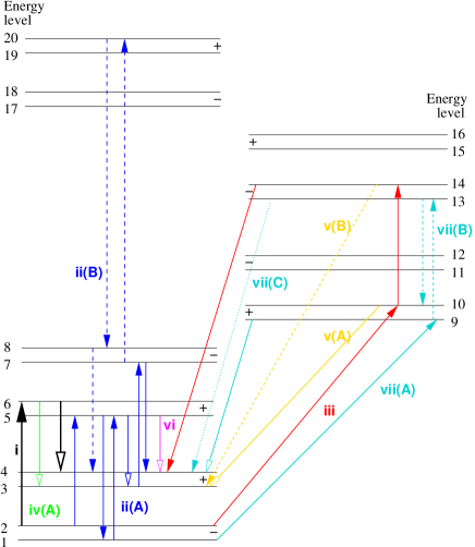
Figure 3: Principal pumping routes for the $1667$ MHz maser under the conditions of Table 2. Markings as for Fig. 2 except that the colour code is extended to seven colours: transitions appearing in Route 4 are drawn in green and then Route 5 in gold, Route 6 in pink and Route 7 in turquoise.

5.1 Summary

The $1667$- and $1665$-MHz pumps share many features: the strongest pair of routes are confined to the ${}^{2}\Pi_{3/2}$ stack of levels, the strongest route does not involve levels higher than the ${}^{2}\Pi_{3/2},J=5/2$ rotational state and the weaker routes make much more extensive use of the ${}^{2}\Pi_{1/2}$ levels. The similarity is particularly striking for the strongest pumping route in each line: for both lines, this consists (considering the forward route only) of a radiative absorption from ${}^{2}\Pi_{3/2},J=3/2$ to ${}^{2}\Pi_{3/2},J=5/2$, followed by a collisional de-excitation back to ${}^{2}\Pi_{3/2},J=3/2$. For $1665$ MHz, the route, in levels, is $1\rightarrow 5$, followed by $5\rightarrow 3$. The analogous route at $1667$ MHz is $2\rightarrow 6$, followed by $6\rightarrow 4$. A similar analogy can be drawn for the second-strongest route in both lines, where a collisional de-excitation is bracketed by a pair and a triplet of radiative lines. The first group operates between the lower halves of the ${}^{2}\Pi_{3/2},J=3/2$ and ${}^{2}\Pi_{3/2},J=5/2$ lambda doublets, and the second group links the upper halves. The swap from the lower to the upper halves is allowed by the intervening collisional de-excitation.

6 The Pumps at a Deeper Level

So far, the present work has derived pumping routes for OH masers in terms of all-process rate-coefficients. Therefore, we know what routes are responsible for most of the steady-state inversion, but some details of the underlying physics are still missing. To proceed, we can expand the all-process rate coefficients presented in eq.(5) - eq.(11) and eq.(12) - eq.(18) in terms of their radiative and collisional parts, so that the importance of routes can be explained in terms of radiation fields and molecular parameters. Some of the expressions are very complex, so I present here the analysis for the most important route at $1665$ MHz, and for its analogue at $1667$ MHz, where the analysis of the pumping schemes leads to a very simple physical understanding.

6.1 1665 MHz

The strongest component of the $1665$ MHz pump is given by the expression in eq.(5). The absolute value of the inversion it generates requires multiplication of $R1$ by the constants outside the main brackets in eq.(2). Here, the only term of interest is the antagonistic part of eq.(5), so we group the denominator with the constants and expand the expression,

$$y=k_{1,5}k_{5,3}-k_{3,5}k_{5,1}$$ (19)

As the $5\rightarrow 3$ transition is radiatively forbidden, expansion of eq.(19) in terms of the radiation field and molecular parameters yields

$$y=(B_{1,5}\bar{J}_{1,5}+C_{1,5})C_{5,3}-C_{3,5}(A_{5,1}+\bar{J}_{1,5}B_{5,1}+C_{5,1})$$ (20)

where $A_{x,y}$, ($B_{x,y}$ ) are Einstein-A (B) coefficients and the $C_{x,y}$ are first-order collisional rate coefficients for population transfer from level $x$ to level $y$. The values of the seven important quantities appearing in eq.(20) are tabulated in Table 3.

Table 3: Radiative and collisional rate coefficients for 1665 MHz

Quantity	Value (Hz)
$A_{5,1}$	$1.24\times 10^{-1}$
$B_{5,1}\bar{J}_{1,5}$	$2.16\times 10^{-2}$
$B_{1,5}\bar{J}_{1,5}$	$3.60\times 10^{-2}$
$C_{5,1}$	$4.35\times 10^{-5}$
$C_{1,5}$	$1.31\times 10^{-6}$
$C_{5,3}$	$3.75\times 10^{-4}$
$C_{3,5}$	$1.13\times 10^{-5}$

It is easy to see from Table 3 that there is a hierarchy of these rate coefficients. The stimulated emission and absorption terms are about five times smaller than the spontaneous emission rate, but of order $100$ times larger than the collisional rate coefficients. A sensible initial simplification of eq.(20) is therefore to ignore terms that are products of collisional coefficients, leaving

$$y\simeq B_{1,5}\bar{J}_{1,5}C_{5,3}-C_{3,5}(A_{5,1}+\bar{J}_{1,5}B_{5,1})$$ (21)

Another glance at Table 3 shows that $C_{3,5}$ is smaller than $C_{5,3}$ by a factor of about $30$. Ignoring the stimulated emission compared with the absorption reduces eq.(21) to

$$y\simeq B_{1,5}\bar{J}_{1,5}C_{5,3}-C_{3,5}A_{5,1}$$ (22)

The Einstein B-value and the upward collisional rate-coefficient can be expressed in terms of the downward expressions, producing

$$y=(C_{5,3}g_{5}/g_{1})[B_{5,1}\bar{J}_{1,5}-A_{5,1}e^{-\frac{h\nu}{kT_{K}}}]$$ (23)

where $g_{1}$ and $g_{5}$ are the statistical weights of levels $1$ and $5$ respectively, $\nu$ is the line-centre transition frequency of the $5\rightarrow 1$ transition, and $T_{k}$ is the kinetic temperature. Expressing the Einstein B-coefficient in terms of the A-coefficient, I obtain

$$y=\frac{A_{5,1}C_{5,3}g_{5}}{g_{1}(e^{\frac{h\nu}{kT_{K}}}-1)}\left[\frac{\bar{J}_{1,5}}{B_{\nu}(T_{K})}-1+e^{-\frac{h\nu}{kT_{K}}}\right]$$ (24)

where $B_{\nu}(T_{K})$ is a Planck function at the local kinetic temperature (for the chosen slab in the ALI model). The group of terms outside the square braket in eq.(24) helps to set the overall speed of the pump, but does not control its direction. For the moment, group these terms as $K$, and noting that the exponential in eq.(24) is vastly smaller than $1$, the final form for $y$ is

$$y\simeq K[(\bar{J}_{1,5}/B_{\nu}(T_{K}))-1]$$ (25)

Two things are responsible for the effectiveness of the pump in eq.(25). The first is that the mean intensity of radiation in the $5\rightarrow 1$ transition must be greater than a Planck function at the same frequency, based on the kinetic temperature. The second is that the energy gap between the ${}^{2}\Pi_{3/2},J=3/2$ and ${}^{2}\Pi_{3/2},J=5/2$ rotational levels is large compared to $kT_{K}$: this condition makes the upward rate coefficient in the collision-only $5\rightarrow 3$ transition much weaker than its downward companion.

The first of these requirements - that the mean intensity exceed the black-body function at the kinetic temperature - can be explained in terms of three physical processes, either singly or in combination. The first is the presence of a radiation field at a temperature higher than $T_{K}$. The ALI model has dust at a temperature $T_{d}=70$ K, so continuum radiation is a possible source of the necessary mean intensity. The second possibility is that radiative transfer effects drive the mean intensity to a level well above what would be expected for LTE at $30$ K, the kinetic temperature. The third possibility is line overlap with another FIR transition. However, in the model used here, the $5\rightarrow 1$ and $6\rightarrow 2$ transitions are not members of the overlapping groups, so the dust continuum and/or NLTE radiation transfer must be responsible.

For the $1665$ MHz pump, I compare the rate $B_{5,1}\bar{J}_{5,1}$ from Table 3 with three other relevant radiative rates. The first of these is the LTE rate, $B_{5,1}B_{\nu}(T_{K})$, which is $2.28\times 10^{-3}$ Hz for $T_{K}=30$ K. The actual rate in the $5\rightarrow 1$ line exceeds this by a factor of $\sim 10$. The second is the black-body rate at the dust temperature, $B_{5,1}B_{\nu}(T_{d})=2.70\times 10^{-2}$ Hz - substantially larger than the actual rate. Thirdly, there is the rate $B_{5,1}S_{1,5}$ generated by the source function in the chosen slab, which has the value $1.97\times 10^{-2}$ Hz. The actual value exceeds this slightly, so the actual radiative rate found in the transition must depend on both a substantial optical depth in the $5\rightarrow 1$ line, and the presence of the dust continuum. This view of the inversion mechanism is consistent with Fig. 1, where there is little or no inversion for models where $T_{d}<T_{K}$.

It is, in fact, possible to give a reasonably detailed physical explanation of the radiative part of the pump, that is to explain eq.(25) in terms of the details of the radiative transfer. The ultimate source of the large mean intensity in the $5\rightarrow 1$ line is the boundary condition on the inner (high optical depth, and the more remote from the observer) boundary of the model. This specifies that the continuum becomes optically thick, and that the abundance of OH falls to zero. As a result, the radiation field at the inner boundary is a Planck function at the (constant) dust temperature, whilst the mean optical depth in the line tends to a large, but finite, value. In the model analysed in the present work, the mean line optical depth reaches $\tau_{M}=265$. All the slabs which make up the numerical model (where $\tau<\tau_{M}$ ) will be referred to here as the line zone. The line zone includes the slab analysed with tracer. Although the line zone also contains dust at the same temperature as the boundary, it is too optically thin to contribute significant radiation to the pumping line. Therefore, it is definitely the boundary which is responsible, and any simplified model can assume that opacity is provided by the line only in the line zone, and by the continuum only in the boundary. High line optical depths ($>150$ ) in the analysed slab and those nearby, suggest that a diffusion approximation may lead to a reasonable physical understanding of the line zone close to the inner boundary.

If a radiation diffusion approximation is assumed (see Appendix C), an analytical solution to the radiation transfer problem can be found. Within the restrictions discussed in the Appendix, the mean intensity in the line zone is given by,

$$\bar{J}(\tau)=B_{\nu}(T_{K})+(B_{\nu}(T_{d})-B_{\nu}(T_{K}))e^{-\sqrt{3\zeta}(\tau_{M}-\tau)}$$ (26)

Equation 26 has sensible limits: the mean intensity tends to a Planck function at the dust temperature as the optical depth approaches the inner boundary, whilst at small optical depth, the limit is a Planck function at the kinetic temperature. Of course eq.(26) has no semblance of validity for small values of $\tau$. Re-arranging eq.(26) to look like eq.(25) yields,

$$\frac{\bar{J}(\tau)}{B_{\nu}(T_{K})}-1=\left(\frac{B_{\nu}(T_{d})}{B_{\nu}(T_{K})}-1\right)e^{-\sqrt{3\zeta}(\tau_{M}-\tau)}$$ (27)

so in the model used in the present work, the boundary value of the bracket ( $10.87$ ) has decayed to $8.496$ over an optical depth shift of $32.4$. This shows that the crucial parameter is $\zeta$. If it were not present in eq.(27), the mean intensity would decay to a value dictated by the kinetic temperature well within the first slab of the line zone, and no pumping radiation would be transported far from the inner boundary. The full definition of $\zeta$, the scattering parameter, is given in Appendix C for a two-level system. However, in the case of the $5\rightarrow 1$ line in the present work, with parameters given in Table 3, it is well approximated by $\zeta\sim C_{5,1}/A_{5,1}=3.51\times 10^{-4}$. This results in an effective optical depth scale thinner than that based on the line-profile mean by a factor of $\sqrt{3\zeta}=0.032$. This scale does not match the decay in $\bar{J}$ found in the model, but this is not surprising given that the diffusion approximation is not strictly valid, and relies on the assumption of a two-level system. The important point is that the effective optical depth scale is vastly thinner than the line scale because of a small value of $\zeta$. The small value of $\zeta$ in turn depends upon the fact that the Einstein A-value in the $5\rightarrow 1$ line is vastly larger than the downward collisional rate coefficient. Any radiation absorbed in this line has a high probability of being re-radiated, in the same line, rather than being collisionally de-excited, which would lead to thermalization of the energy. A large fraction of the absorption therefore behaves effectively as scattering, so that the effects of the boundary continuum on pumping can be felt in the slab studied with tracer, and indeed substantially closer to the observer.

It is perhaps worth noting that photons travelling directly from the boundary do not actually penetrate very far into the model. This radiation also does not decay exponentially as $\tau_{M}-\tau$, because the wings of the Gaussian line profile are always substantially optically thinner than the line mean. Very roughly, the actual inner boundary radiation penetrates as $1/(\tau_{M}-\tau)$, for optical depth shifts $>1$, so it would have only a marginal effect on the slab studied in the present work, when compared to the ‘effectively scattered’ radiation discussed above.

An interesting rider to this investigation of the leading $1665$-MHz pump is to consider the symmetry between the routes linking levels $3$ and $1$ via level $5$, as discussed above, and those linking levels $3$ and $1$ via level $7$. If one assumes similar Einstein coefficients and collisional rate coefficients, one would conclude that a radiative excitation from level $3$ to level $7$, followed by a collisional decay from $7$ to level $1$, would provide an anti-inverting mirror to the similar transitions via level $5$, negating the inverting effect of the latter. The reason that this does not happen in the model discussed here is that the downward rate-coefficient, $C_{7,1}=5.00\times 10^{-5}$ Hz, is considerably smaller (by a factor of $0.133$ ) than $C_{5,3}$ (see Table 3). Importantly, $C_{5,3}$ is the largest term in the tracer expansion of $k_{5,3}^{6}$, which follows from eq.(5), and the fact that the $5\rightarrow 3$ transition is radiatively forbidden. Therefore, direct collisional transfer in this route exceeds all indirect methods of transfer between levels $5$ and $3$, and the large difference between $C_{5,3}$ and $C_{3,5}$ is significant in creating inversion. By contrast, $C_{7,1}$ is only the third most important route in the expansion of $k_{7,1}^{8}$. It is exceeded in importance by radiative routes transfering population from level $7$ to level $1$ via levels in the ${}^{2}\Pi_{1/2}$ stack. Therefore, compared with $5\rightarrow 3$, direct collisional transfer between level $7$ and level $1$ plays a much less prominent role, and the difference between $C_{1,7}$ and $C_{7,1}$, though large, is unimportant as an anti-inverting mechanism.

At a still deeper level, it is possible to explain why the collisional rate coefficient $C_{7,1}$ is so much smaller than $C_{5,3}$: both coefficients are constructed from contributions due to collisions with ortho- and para-H₂. The rate coefficients from collisions of OH with ortho-H₂ are similar for both transitions, with the coefficient for $7\rightarrow 1$ stronger by a factor of $1.08$. However the rate coefficients for the two transitions derived from collisions with para-H₂ are very different. This ‘parity propensity’ of the OH plus para-H₂ collision cross sections was noted by Offer et al. [1994]. In fact, the ratio of the rate coefficients for the $5\rightarrow 3$ and $7\rightarrow 1$ transitions, due to collisions with para-H₂, is $8.37$ at the $30$ K kinetic temperature of the model. The strong parity propensity of the collisions with para-H₂ is apparent at this temperature because the equilibrium abundance of the ortho-H₂ is small (about $2.5$ per cent). At higher temperatures, the abundance of ortho-H₂ would be expected to rise, and the efficiency of the pump to fall, as the ortho- to para-H₂ abundance ratio tends towards its high-temperature value of $3$. A glance at Fig. 1 suggests that this is indeed the case, with the pumping mechanism becoming ineffective below a kinetic temperature of $100$ K, where the ratio of the contributions of the ortho- and para-hydrogen species to the overall rate coefficient is $1.5$.

6.2 1667 MHz

The strongest pump route at $1667$ MHz can be analysed in a very similar way to the $1665$ MHz route discussed above. The inversion expression to be expanded is

$$y^{\prime}=k_{2,6}k_{6,4}-k_{4,6}k_{6,2}$$ (28)

and the version of eq.(28) fully expanded in terms of molecular parameters and the radiation field in transition $2\rightarrow 6$ is

$$y^{\prime}=(B_{2,6}\bar{J}_{2,5}+C_{2,6})C_{6,4}-C_{4,6}(A_{6,2}+\bar{J}_{2,6}B_{6,2}+C_{6,2})$$ (29)

Values of the various terms appearing in eq.(29) appear in Table 4.

Table 4: Radiative and collisional rate coefficients for 1667 MHz

Quantity	Value (Hz)
$A_{6,2}$	$1.38\times 10^{-1}$
$B_{6,2}\bar{J}_{2,6}$	$2.31\times 10^{-2}$
$B_{2,6}\bar{J}_{2,6}$	$3.24\times 10^{-2}$
$C_{6,2}$	$5.16\times 10^{-5}$
$C_{2,6}$	$1.30\times 10^{-6}$
$C_{6,4}$	$4.74\times 10^{-4}$
$C_{4,6}$	$1.20\times 10^{-5}$

Following through the same steps as for $1665$ MHz, the final expression for $y^{\prime}$ is

$$y^{\prime}\simeq K^{\prime}[(\bar{J}_{2,6}/B_{\nu}(T_{K}))-1]$$ (30)

It can be shown that the mean intensity in the $2\rightarrow 6$ line which pumps $1667$ MHz is actually smaller than the corresponding mean intensity in the $1\rightarrow 5$ transition. On this basis $y^{\prime}$ in eq.(30) would be expected to be smaller than $y$ for the case of identical constants $K=K^{\prime}$. The reason that the $1667$ MHz inversion is larger, per sublevel, by a factor of $1.188$ therefore requires that either $K>K^{\prime}$, or that the inversion ratio is explained by differences in the external constants appearing in eq.(2) and eq.(3). If we take the inversion per sublevel, then the ratio of the external constants is

$$R_{ext}=\frac{\Delta\rho_{42}}{\Delta\rho_{31}}=\frac{3(k_{1,1}^{5}k_{3,3}^{5}-k_{1,3}^{5}k_{3,1}^{5})}{5k_{2,2}^{4}k_{4,4}^{5}}$$ (31)

When evaluated, $R_{ext}=1.093$. Therefore, part of the reason for the larger inversion at $1665$ MHz lies in the ratio of the constants, $R_{c}=K^{\prime}/K$. Ignoring the exponential terms, the ratio of which is $1.0$ to better than one part in $10^{4}$, $R_{c}$ is given by

$$R_{c}=\frac{A_{6,2}C_{6,4}g_{6}g_{1}}{A_{5,1}C_{5,3}g_{2}g_{5}}$$ (32)

which evaluates to $R_{c}=1.1794$. One reason why the inversion at $1667$ MHz is larger than the corresponding inversion at $1665$ MHz is therefore that both transitions in its strongest pumping routes are faster than their analogues in the $1665$ MHz pump. For comparison of the Einstein A-values and collisional rate coefficients, see Table 4 and Table 3. The radiative part of the pump for $1667$ MHz depends on the efficient transfer of radiation from the inner boundary of the model by effective scattering of radiation in the $6\rightarrow 2$ line in a very similar manner to the detailed discussion for $1665$ MHz, given in Section 6.1.

The similarity of the $1667$- and $1665$-MHz pumps also extends to the symmetry breaking between the pumping route (level $2$ to level $4$ via level $6$) investigated above, and its anti-inverting mirror, taking population from level $4$ to level $2$ via level $8$. Just as in the case of the $1665$-MHz pump, the inverting route has the direct collisional transfer as the leading term in the tracer expansion of its downward transition ( $6\rightarrow 4$ in this case), but the direct transfer is relatively unimportant in the downward transition ( $8\rightarrow 2$ ) of the anti-inverting route. The weakness of the direct $8\rightarrow 2$ collisional transfer is based on the size of the collisional rate coefficient ($C_{8,2}/C_{6,4}=0.18$), which in turn depends on the overwhelming contribution of the para-H₂ species, with its large parity propensity, to collisions at low temperatures.

7 Efficiencies

I discuss here the efficiency of overall schemes and the efficiencies of important individual routes. I define the efficiency of a scheme or route as the ratio of the rate at which it produces inversion divided by the total population flow rate through the same scheme or route. For example, considering the overall $1665$ MHz pumping scheme, there are the direct and indirect terms from eq.(2). For the direct part of the pump, the efficiency is

$$\epsilon_{d}=\frac{k_{1,3}^{4}-k_{3,1}^{4}}{k_{1,3}^{4}+k_{3,1}^{4}}$$ (33)

which evaluates to $4.1$ per cent. Similarly, the indirect part of the pump is $3.34$ per cent efficient. Weighting these two efficiencies by the contribution each makes to the inversion, the overall efficiency of the $1665$ MHz pump is $3.75$ per cent. In the case of the $1667$ MHz pump, obtaining the overall efficiency is a little more laborious, but still straightforward, and the mean of all the routes in eq.(3), weighted by contribution to the inversion gives an efficiency of $4.60$ per cent. The third term in the brackets of eq.(3) is notable in having the largest individual efficiency, of $5.13$ per cent. Overall, the $1667$ MHz pump is the more efficient, which is unsurprising, since the inversion in this line is also the larger.

7.1 individual routes

Individual routes within the overall scheme can have substantially higher efficiencies than those for the scheme as a whole. I define such internal efficiencies as those calculated for a route when the denominator is confined to consideration of that route only. For example, the strongest pumping route at $1665$ MHz has the internal efficiency,

$$\epsilon_{R1}=\frac{k_{1,5}k_{5,3}-k_{3,5}k_{5,1}}{k_{1,5}k_{5,3}+k_{3,5}k_{5,1}}$$ (34)

which has the numerical value of $78.2$ per cent. The analagous route in the $1667$ MHz system, operating via levels $2$, $6$ and $4$ is internally $77.6$ per cent efficient. These figures drop to $\sim 2.5$ per cent when the routes are expressed as part of the expansion of eq.(33), or its $1667$ MHz analogue. Routes with many links are not noticeably less efficient. For example, Route 2B in the $1665$ MHz scheme, which climbs to level $20$ in the ${}^{2}\Pi_{3/2},J=7/2$ rotational level, has the internal efficiency

$$\epsilon_{R2B}=\frac{k_{1,5}k_{5,2}k_{2,6}k_{6,4}k_{4,8}k_{8,20}k_{20,7}k_{7,3}-\Omega_{2B}}{k_{1,5}k_{5,2}k_{2,6}k_{6,4}k_{4,8}k_{8,20}k_{20,7}k_{7,3}+\Omega_{2B}}$$ (35)

with the numerical value of $77.0$ per cent.

8 Discussion

The results reported here and in Gray et al. [2005] show that it is possible to trace pumping schemes in OH in considerable detail in at least two of the common OH-maser environments (Galactic star-forming regions and evolved-star envelopes). The pumping schemes revealed so far are actually very complex, but a large proportion of their inverting strength can be explained in terms of a few dominant routes. An obvious extension of this work is to study the additional ground-state OH maser environments: OH megamasers and those supernova remnants which support strong masing at $1720$ MHz. Additional work needs to be done to confirm the generality of the schemes analysed in the present work, both in terms of the spatial variation within one model, and variation between models with different input parameters. To complete such an analysis of many schemes in a reasonable time requires considerably improved automation of the population tracing process. The explanation of the radiative part of the pump in terms of the transport of radiation from the optically thick boundary to a significant part of the model (many slabs) by means of a modifed optical depth scale does at least suggest that the same pumping mechanism operates within a large fraction of the current geometrical model.

The importance of parity propensity in collisions between OH and para-H₂ in the pumping scheme for both OH main lines means that the ortho- to para-H₂ ratio in the gas of the maser zone must be well biased in favour of the para-species for the schemes investigated here to operate efficiently. Given that H₂ forms in the ratio of 3:1 in favour of the ortho-form, as dictated by the nuclear spin statistics, maser action via the pumping schemes discussed here would require time for the species ratio to move substantially towards the thermodynamic ratio via a set of proton exchange reactions [2006]. In some circumstances the timescale for these reactions could equate to the ‘switch-on’ time for main-line OH masers.

Labelling of energy levels is of course arbitrary, so expressions similar to eq.(2) and eq.(3) can be formed for excited-state inversions without increased complexity, providing that, say, the ${}^{2}\Pi_{3/2},J=5/2$ levels were labelled $1-4$ instead of those in the ${}^{2}\Pi_{3/2},J=3/2$ ground state. It would then be possible to trace the common $6030$ and $6035$ MHz inversions; alternative re-labelling would allow tracer to be applied to any of the other OH rotational levels that support maser action. A likely problem with the extension of the method to excited states is one of stability: the elimination process following the naive method relies on the last levels eliminated having large populations as a form of numerical pivoting. There may, however, be ways of avoiding these stability problems by attaching the operation log to the basic numerical method, provided that the interpretation in terms of rate coefficients can be preserved.

It may also be possible to extend this inversion-tracing method to molecules other than OH. In many interesting cases, such as the $22$ GHz maser line of water, the maser levels lie well above the ground state, so any attempts at analysis would suffer from the stability problems already discussed in connexion with the excited rotational states of OH. However, there may be an even more fundamental barrier to understanding inversions in some cases. In the case of methanol [1994a] the authors show that, for the $2_{0}-3_{-1}$ Class II maser transition of the E-species, $65$ per cent of the maser flux results from pumping cycles with a number of links which exceeds $10$. In these cases at least, it is almost certainly not possible to write down a manageable expression for the inversion: either the number of required terms would be too great, or the expressions too complicated, or both. If the tracer method is to be extended to another molecule, the first one to try is probably SiO: it has a relatively simple level structure, and a maser (though not one of the strongest or most common) has been observed between the lowest two rovibrational levels ($v=0,J=1-0$). In addition, population in each vibrational level tends to be concentrated towards the lower rotational levels, which is likely to aid numerical stability.

Another application which is likely to prove fruitful is to extend the tracer method to saturating conditions. The semi-classical analysis by Field & Gray [1988] automatically breaks the kinetic scheme into coefficients which multiply the maser radiation and those which do not. The former affect the inversion as the maser saturates, whilst the latter generate the inversion, like those studied in the present work. Both sets of coefficients in models (for example Gray, Field & Doel [1992]) are generated in a very similar manner, and, for the ground-state OH masers, would introduce no extra stability problems. The coefficients that multiply the maser intensity could be studied as a function of propagation distance along the maser, showing how the increasingly rapid transfer of population across the maser levels introduces newly important transfer routes.

9 Conclusions

I conclude that it is possible to trace the population transfer routes which cause strong inversions in the $18$ cm OH main-line masers under conditions typical of star-forming regions. The number of routes which need to be traced in order to recover the great majority of the inversion is modest - a conclusion which does not necessarily hold for the kinetic schemes of other molecules, or even for OH in other environments.

The pumping schemes derived for the $1665$- and $1667$-MHz lines show strong similarity, and are biased quite strongly to the ${}^{2}\Pi_{3/2}$ stack of rotational levels, unlike the case of $1612$ MHz OH masers in late-type stellar atmospheres. In both lines, the strongest route contains just two transitions, comprising, for the forward route, a radiative absorption, lifting population to the ${}^{2}\Pi_{3/2},J=5/2$ rotational state, followed by collisional de-excitation to the upper part of the ground-state lambda doublet. This inclusion of a radiatively forbidden link to switch from the lower to the upper half of the lambda-doublet system is also employed by the next most important pumping route in both main lines. Anti-inverting ‘mirror’ transitions are not effective because of the parity propensity found in collisions between OH and para-H₂.

The effectiveness of these routes in the ${}^{2}\Pi_{3/2}$ stack is based firstly upon the fact that the energy gap between the ${}^{2}\Pi_{3/2},J=3/2$ and ${}^{2}\Pi_{3/2},J=5/2$ rotational states is large compared to the energy equivalent of the kinetic temperature, which favours collisional de-excitation over excitation, and secondly on the presence of a dust radiation field which has a characteristic temperature which is locally hotter than the kinetic temperature, a result of efficient transfer of radiation from the optically thick boundary by ‘effective scattering’.

ACKNOWLEDGMENTS

MDG acknowledges PPARC for financial support under the UMIST astrophysics 2002-2006 rolling grant, number PPA/G/O/2001/00483, and thanks the referee for helpful suggestions regarding the improvement of the later parts of the paper.

Appendix A Diagonal Coefficients

The aim of this section is to prove that a diagonal coefficient, $k_{j,j}^{p}$, at elimination stage $p$ is equal to the sum of the all-process rate-coefficients from level $j$ to all the un-eliminated levels, or

$$k_{j,j}^{p}=\sum_{m=1;m\neq j}^{p-1}k_{j,m}^{p}$$ (36)

This is true by definition for the original matrix ($p=N+1$), but is not obviously so for any smaller value of $p$.

The state of the set of kinetic master equations at elimination stage $p$ looks like:

$$\begin{array}[]{ccccccr}k_{p-1,p-1}^{p}\rho_{p-1}\!\!\!\!&\!\!\!\!...\!\!\!\!&\!\!\!...&\!\!\!\!\!\!...\!\!\!\!&\!\!\!-k_{i,p-1}^{p}\rho_{i}\!\!\!\!&\!\!\!\!\!\!\!\!\!...\!\!\!\!\!&\!\!\!\!\!-k_{1,p-1}^{p}\rho_{1}\!=\!0\\ -k_{p-1,p-2}^{p}\rho_{p-1}\!\!\!\!&\!\!\!\!...\!\!\!\!&\!\!\!...&\!\!\!\!\!\!...\!\!\!\!&\!\!\!-k_{i,p-2}^{p}\rho_{i}\!\!\!\!&\!\!\!\!\!\!\!\!\!...\!\!\!\!\!&\!\!\!\!\!-k_{1,p-2}^{p}\rho_{1}\!=\!0\\ \vdots\!\!\!\!&\!\!\!\!...\!\!\!\!&\!\!\!...&\!\!\!\!\!\!...\!\!\!\!&\!\!\!...\!\!\!\!&\!\!\!\!\!\!\!\!\!...\!\!\!\!\!&\!\!\!\!\!\vdots=\!0\!\\ -k_{p-1,j}^{p}\rho_{p-1}\!\!\!\!&\!\!\!\!...\!\!\!\!&\!\!\!+k_{j,j}^{p}\rho_{j}&\!\!\!\!\!\!...\!\!\!\!&\!\!\!-k_{i,j}^{p}\rho_{i}\!\!\!\!&\!\!\!\!\!\!\!\!\!...\!\!\!\!\!&\!\!\!\!\!-k_{1,j}^{p}\rho_{1}=\!0\!\\ \vdots\!\!\!\!&\!\!\!\!...\!\!\!\!&\!\!\!...&\!\!\!\!\!\!...\!\!\!\!&\!\!\!...\!\!\!\!&\!\!\!\!\!\!\!\!\!...\!\!\!\!\!&\!\!\!\!\!\vdots=\!0\!\\ -k_{p-1,2}^{p}\rho_{p-1}\!\!\!\!&\!\!\!\!...\!\!\!\!&\!\!\!...&\!\!\!\!\!\!...\!\!\!\!&\!\!\!...\!\!\!\!&\!\!\!\!\!\!\!\!\!+k_{2,2}^{p}\rho_{2}\!\!\!\!\!&\!\!\!\!\!-k_{1,2}^{p}\rho_{1}=\!0\!\\ k_{p-1,1}^{p*}\rho_{p-1}\!\!\!\!&\!\!\!\!...\!\!\!\!&\!\!\!...&\!\!\!\!\!\!...\!\!\!\!&\!\!\!...\!\!\!\!&\!\!\!\!\!\!\!\!\!+k_{2,1}^{p*}\rho_{2}\!\!\!\!\!&\!\!\!\!\!+k_{1,1}^{p*}\rho_{1}\!=\!{\cal N}\\ \end{array}$$ (37)

where $\rho_{x}$ is the population of level $x$ and the conservation equation coefficients, written with a star in the superscript, appear in the final equation. An additional equation is now eliminated by the naive method: the topmost equation in the set eq.(37) is used to eliminate $\rho_{p-1}$, such that

$$\rho_{p-1}=(\sum_{m=1}^{p-2}k_{m,p-1}^{p}\rho_{m})/k_{p-1,p-1}^{p}$$ (38)

and this population is eliminated from all the others in favour of the expression in eq.(38). Concentrating on the arbitrary equation $j$ such that $j\leq p-2$, the diagonal coefficient in this equation is modified to the form

$$k_{j,j}^{p-1}=k_{j,j}^{p}-\frac{k_{p-1,j}^{p}k_{j,p-1}^{p}}{k_{p-1,p-1}^{p}}$$ (39)

I now assume that the desired result is true at elimination stage $p$, and prove by induction that it is true at all further stages with $p>2$, noting that at $p=3$, only a trivial $2\times 2$ matrix remains. This assumption allows the development of eq.(39) to

$$k_{j,j}^{p-1} = k_{j,1}^{p}+...+k_{j,j-1}^{p}+k_{j,j+1}^{p}+...+k_{j,p-1}^{p}$$ (40)

$$- k_{p-1,j}^{p}k_{j,p-1}^{p}/k_{p-1,p-1}^{p}$$

I now add zero to each term on the right-hand side of eq.(40), but in a form which allows development of the off-diagonal coefficients. Equation 40 becomes,

$$k_{j,j}^{p-1} = k_{j,1}^{p}+\frac{k_{j,p-1}^{p}k_{p-1,1}^{p}}{k_{p-1,p-1}^{p}}-\frac{k_{j,p-1}^{p}k_{p-1,1}^{p}}{k_{p-1,p-1}^{p}}$$

$$+ ... +k_{j,j-1}^{p}+\frac{k_{j,p-1}^{p}k_{p-1,j-1}^{p}}{k_{p-1,p-1}^{p}}-\frac{k_{j,p-1}^{p}k_{p-1,j-1}^{p}}{k_{p-1,p-1}^{p}}$$

$$+ k_{j,j+1}^{p}+\frac{k_{j,p-1}^{p}k_{p-1,j+1}^{p}}{k_{p-1,p-1}^{p}}-\frac{k_{j,p-1}^{p}k_{p-1,j+1}^{p}}{k_{p-1,p-1}^{p}}$$

$$+ ... +k_{j,p-2}^{p}+\frac{k_{j,p-1}^{p}k_{p-1,p-2}^{p}}{k_{p-1,p-1}^{p}}-\frac{k_{j,p-1}^{p}k_{p-1,p-2}^{p}}{k_{p-1,p-1}^{p}}$$ (41)

$$+ k_{j,p-1}^{p}-\frac{k_{j,p-1}^{p}k_{p-1,j}^{p}}{k_{p-1,p-1}^{p}}$$

and the off-diagonal coefficients are now of a form which can be upgraded to the next elimination stage via eq.(1). The coefficient at level $p$ combines with the positive fraction on each line (except the last) to form a coefficient at stage $p-1$, leaving

$$k_{j,j}^{p-1} \!=\! k_{j,1}^{p-1}+...+k_{j,j-1}^{p-1}+k_{j,j+1}^{p-1}+...+k_{j,p-2}^{p-1}+k_{j,p-1}^{p}$$ (42)

$$\!-\! \frac{k_{j,p-1}^{p}}{k_{p-1,p-1}^{p}}\left(k_{p-1,1}^{p}+...+k_{p-1,j-1}^{p}\right.$$

$$\!+\! \left.k_{p-1,j+1}^{p}+...+k_{p-1,p-2}^{p}+k_{p-1,j}^{p}\right)$$

where a common factor of $k_{j,p-1}^{p}/k_{p-1,p-1}^{p}$ has been extracted from the negative terms on the right-hand side of eq.(41). I now note that the bracket in eq.(42) is the sum of all the rate coefficients taking population out of level $p-1$, and is therefore equal to the diagonal coefficient $k_{p-1,p-1}^{p}$, given the assumption about such coefficients at elimination stage $p$. The bracket therefore cancels with this coefficient in the denominator, leaving two coefficients of the form $k_{j,p-1}^{p}$ with opposite signs. Cancellation of these leaves

$$k_{j,j}^{p-1}=\sum_{m=1;m\neq j}^{p-2}k_{j,m}^{p-1}$$ (43)

which is of the form of eq.(36), but with $p$ replaced by $p-1$. Therefore, if the initial assumption is true for any given stage of elimination, it remains true for the next. As it is true by definition for the original set of equations, where $p=N+1$, then the assumption is true for all subsequent eliminations at least as far as $p=3$.

Appendix B Denominator

This section shows that the external denominator ($D$ in eq.(2) and eq.(3)) is positive definite. In terms of rate coefficients evaluated at elimination stage $p=4$, the denominator is given by

$$D = k_{3,3}^{4}(k_{1,1}^{4*}k_{2,2}^{4}+k_{1,2}^{4}k_{2,1}^{4*})+k_{3,1}^{4*}(k_{1,3}^{4}k_{2,2}^{4}+k_{1,2}^{4}k_{2,3}^{4})$$ (44)

$$+ k_{3,2}^{4}(k_{1,3}^{4}k_{2,1}^{4*}-k_{1,1}^{4*}k_{2,3}^{4})$$

where coefficients marked with an asterisk in the superscript (starred) come from the conservation equation,

$$\sum_{i=1}^{p-1}k_{i,1}^{p*}\rho_{i}={\cal N}$$ (45)

and cannot be interpreted in the same manner as the other rate-coefficients via eq.(1). At $p=N+1$, these starred coefficients are all equal to $1.0$ and subsequent actions can only add combinations of positive-definite rate-coefficients to them. They are therefore positive definite at any value of $p$. Given this result, and the proof in Appendix A, the middle term in eq.(44) is positive definite, and will be called $B$. Using the result of Appendix A to expand $k_{3,3}^{4}=k_{3,1}^{4}+k_{3,2}^{4}$, eq.(44) becomes

$$D \!\!\!\!\!=\!\!\!\!\! k_{3,1}^{4}k_{1,1}^{4*}k_{2,2}^{4}+k_{3,1}^{4}k_{1,2}^{4}k_{2,1}^{4*}+k_{3,2}^{4}k_{1,1}^{4*}k_{2,2}^{4}+k_{3,2}^{4}k_{1,2}^{4}k_{2,1}^{4*}$$ (46)

$$\!\!\!\!\!+\!\!\!\!\! B+k_{3,2}^{4}k_{1,3}^{4}k_{2,1}^{4*}-k_{3,2}^{4}k_{1,1}^{4*}k_{2,3}^{4}$$

following the expansion of the first and third brackets of eq.(44). The first, second and fourth terms of eq.(46), and the first term following $B$, are all positive definite, and may be combined as $A$. This leaves,

$$D=A+k_{3,2}^{4}k_{1,1}^{4*}k_{2,2}^{4}+B-k_{3,2}^{4}k_{1,1}^{4*}k_{2,3}^{4}$$ (47)

but when $k_{2,2}^{4}$ is expanded in accordance with Appendix A, it contains $k_{2,3}^{4}$, so the remaining negative term in eq.(47) is cancelled exactly, and $D$ is positive definite.

Appendix C Radiation Diffusion

In a zone where radiation transfer is diffusive, application of the Eddington approximation (see for example Rybicki & Lightman [1979]) leads to a radiation diffusion equation for the mean intensity of the form,

$$\frac{d^{2}\bar{J}}{d\tau^{2}}=3\zeta(\bar{J}(\tau)-B_{\nu}(\tau)),$$ (48)

where $B_{\nu}(\tau)$ is a the Planck function at the kinetic temperature, and the source function has been elimated in favour of the mean intensity, using the standard expression from molecular kinetics,

$$\bar{S}(\tau)=\zeta(\tau)B_{\nu}(\tau)+(1-\zeta(\tau))\bar{J}(\tau).$$ (49)

I note that eq.(49) implicity assumes a two-level model: in the many-level case, the multiplier of $\bar{J}$ cannot be represented as $1-\zeta$, and both this multiplier and $\zeta$ depend on the mean intensities and molecular parameters of all other radiative and collisionally allowed transitions. In the two-level case, the parameter $\zeta$ is independent of optical depth if the kinetic temperature is constant, and is given by

$$\zeta=\frac{g_{u}C_{u,l}-g_{l}C_{l,u}}{g_{u}C_{u,l}-g_{l}C_{l,u}+g_{u}A_{u,l}}$$ (50)

where $u$ is the upper and $l$, the lower level of the transition. As elsewhere in the paper, $C_{u,l}$ ( $C_{l,u}$ ) is the downward (upward) collisional rate coefficient, $A_{u,l}$ is the Einstein A-coefficient and $g_{u}$, $g_{l}$ are statisical weights.

References

- [1984] Andresen P., Hausler D., Lülf H.W., 1984, A&A, 138, 17
- [1980] Bujarrabal V., Guibert J., Nguyen-Q-Rieu, Omont A., 1980, A&A, 84, 311
- [1991] Cesaroni R., Walmsley C.M., 1991, A&A, 241, 537
- [1993] Collison A.J., Nedoluha G.E., 1993, ApJ, 413, 735
- [1994] Collison A.J., Nedoluha G.E., 1994, ApJ, 422, 193
- [1977] Destombes J.L., Marlière C., Baudry A., Brillet J., 1977, A&A, 60, 55
- [1987] Dickinson D.F., 1987, ApJ, 313, 408
- [1985] Dixon R.N., Field D., Zare R.N., 1985, Chem. Phys. Lett., 122, 310
- [1981] Elitzur M., 1981, in ‘Physical Processes in Red Giants’ (I. Iben & A. Renzini, eds.), Reidel, Dordrecht, p363
- [1976] Elitzur M., Goldreich P., Scoville N., 1976, ApJ, 205, 384
- [1988] Field D., Gray M.D., 1988, MNRAS, 234, 353
- [2006] Flower D.R., Pineau des Forêts G., Walmsley C.M., 2006, A&A, 449, 621
- [1987] Gaume R.A., Mutel R.L., 1987, ApJSS, 65, 193
- [2001] Gray M.D., 2001, MNRAS, 324, 57
- [1991] Gray M.D., Doel R.C., Field D., 1991, MNRAS, 252, 30
- [1992] Gray M.D., Field D., Doel R.C., 1992, A&A, 262, 555
- [2005] Gray M.D., Howe, D.A., Lewis, B.M., 2005, MNRAS, 364, 783
- [1994] Jones K.N., Field D., Gray M.D., Walker R.N.F., 1994, A&A, 288, 581
- [1990] Kylafis N.D., Norman C.A., 1990, ApJ, 350, 209
- [1969] Litvak M., 1969, ApJ, 156, 471
- [1980] Lucas R., 1980, A&A, 84, 36
- [1994] Offer A.R., van Hemmert M.C., van Dishoeck E.F., 1994, J. Chem. Phys., 100, 362
- [1996] Pavlakis K.G., Kylafis N.D., 1996, ApJ, 467, 309
- [1989] Piehler G., Kegel W.H., 1989, A&A, 214, 339
- [1995] Randell J., Field D., Jones K.N., Yates J.A., Gray M.D., 1995, A&A, 300, 659
- [1979] Rybicki G.B., Lightman A.P., 1979, ‘Radiative Processes in Astrophysics’, Wiley, New York
- [1985] Scharmer G.B., Carlsson M., 1985, J. Comp. Phys. 59, 56
- [1986] Sobolev A.M., 1986, Sov. Ast. 30, 399
- [1989] Sobolev A.M., 1989, Astronomische Nachrichten, 310, 343
- [1994a] Sobolev A.M., Deguchi S., 1994, ApJ, 433, 719
- [1994b] Sobolev A.M., Deguchi S., 1994, A&A, 291, 569
- [1992] Stift M.J., 1992, Lecture Notes in Physics, 401, 431
- [1997] Yates J.A., Field D., Gray M.D., 1997, MNRAS, 285, 303
- [2005] Yu Z., 2005, Annals of Shanghai Observatory (English abstract), 26, 95