Holography and the scale-invariance of density fluctuations

Abstract

We study a scenario for the very early universe in which there is a fast phase transition from a non-geometric, high temperature phase to a low temperature, geometric phase described by a classical solution to the Einstein equations. In spite of the absence of a classical metric, the thermodynamics of the high temperature phase may be described by making use of the holographic principle. The thermal spectrum of fluctuations in the high temperature phase manifest themselves after the phase transition as a scale invariant spectrum of fluctuations. A simple model of the phase transition confirms that the near scale invariance of the fluctuations is natural; but the model also withstands detailed comparison with the data.

In this letter we propose a new hypothesis about the very early universe in which the notion of holography plays a key role. We will see that it gives rise to a scale invariant distribution of density fluctuations, without invoking inflation. This hypothesis is inspired by a scenario that has been proposed recently non-geometry in which the universe begins in a high temperature phase (Phase I) which is not described in terms of fields on classical spacetime manifolds; rather it has a non-geometrical, purely quantum mechanical description, which can be expressed simply in terms of the holographic principle. The spacetime geometry is created in a phase transition, into Phase II, in which it is appropriate to describe the universe to a decent approximation in terms of fields or other degrees of freedom (particles, strings, etc) moving in a classical background geometry. (This may be called geometrogenesis). The phase transition happens at temperature $T_{c}$ and is abrupt (in a sense to be made precise later) and imprints on Phase II a spectrum of thermal fluctuations which arise in Phase I.

The innovation in this paper is to use the holographic principle to characterize the two phases. That principle, as enunciated by ’t Hooft thooft , asserts that any region of space bounded by a surface $\cal S$ of area $A$ can be described by a finite number of degrees of freedom given by $N={A}/(4G\hbar)$. These evolve according to a fundamental dynamics, given by Hamiltonian $H$. The term “holography” has also acquired other different meanings susk , but we stress that we use it in its original sense otherholo .

To describe classical physics there must be non-local correlations among the degrees of freedom on the surface, so as to make it appear that the dynamics is local in a volume $V$ described by a classical geometry in a region $\cal R$ that $\cal S$ bounds. Close to the ground state we expect that $V\approx A^{\frac{3}{2}}$ whenever the curvature can be neglected. But in Phase I there is not yet a classical spacetime geometry. We propose that this phase be then characterized as an disordered phase, which means that the non-local correlations which are needed on the surface to construct the illusion of local three dimensional physics are not yet established, and are peculiar to Phase II. At the same time, the degrees of freedom in Phase I are highly interconnected, as in the model of non-geometry and so reach equilibrium before the phase transition. This solves the horizon problem, as noted in non-geometry ; the next challenge is to generate an almost scale invariant spectrum of fluctuations.

Our idea is very simple, and even though we’ll derive it step by step later, we sketch it first. If Phase I is in thermal equilibrium we expect that the $N$ (local) fundamental degrees of freedom are excited to energy $T$. Thus, in this disordered phase the holographic principle implies that $E=NT=\frac{A}{4\hbar G}T$; that is, for $T>T_{c}$ the specific heat at fixed ${\cal R}$ is $c_{\cal R}={\partial E\over\partial T}=N$, which scales like the area. A well known result tells us that the thermal fluctuations in the energy contained in a fixed region are given by $\sigma^{2}_{E}=T^{2}c_{\cal R}$. Therefore in Phase I we have $\sigma^{2}_{E}\approx{T^{2}\over 4\hbar G}A$, and because this scales like $A$ (instead of $V$, as usual) we have a scale-invariant spectrum of fluctuations, rather than the usual white noise. If the phase transition is “fast”, when the classical metric emerges in Phase II these fluctuations propagate to the potential. Most modes are now outside the Hubble radius, so we end up with a scale-invariant spectrum of adiabatic density fluctuations, with amplitude fixed by the ratio $T_{c}/T_{Pl}$.

We shall proceed as follows. We first present a description of the two phases, justified by basic facts of the quantum theory of gravity, and compute the associated density fluctuations. We next propose a scenario for the generation of classical geometry during the transition. This results in a scale invariant distribution of fluctuations outside the horizon of the classical geometry that emerges at the end of the transition. We then devote some time to weakening our hypotheses, showing how the essential results apply to a large class of models of this type. Finally we quantify departures from scale-invariance, predicting the amplitude, spectral index, and its running in terms of $T_{c}$, and $\gamma$, the critical exponent characterizing the phase transition. A comparison with other models and a word on tensor modes closes this Letter.

To characterize the two phases in more detail we must make a few general assumptions. Firstly, that the universe can be described at all times as having fixed three dimensional spatial topology, but not necessarily a fixed classical metric. Secondly, that the physics in any region $\cal R$ can be described in a hamiltonian formulation in terms of a Hilbert space ${\cal H}_{\cal R}$. $\cal R$ has a boundary $\partial{\cal R}={\cal S}$. And finally that among the operators in ${\cal H}_{\cal R}$ are $\hat{A}$, the area of ${\cal S}$, the hamiltonian constraint $\cal C$ and diffeomorphism constraints $\cal D$ and a boundary contribution to the hamiltonian $\hat{h}=\int_{\cal S}\hat{\mu}$ where $\hat{\mu}$ is a local operator on the boundary. The total hamiltonian for quantum spacetime and matter in $\cal R$ is then,

$$\hat{H}=\int_{\cal S}\hat{\mu}+\int_{\cal R}N{\cal C}+v^{a}{\cal D}_{a}$$ (1)

The quantum states of interest are physical states that are in the kernel of $\cal C$ and $\cal D$. These assumptions are common to many approaches to quantum gravity as they follow just from diffeomorphism invariance.

We then hypothesize that there are two different kinds of solutions to the quantum constraints which each characterize one of the phases. We characterize Phase II as being ordered three dimensionally. This means that there is a classical non-degenerate three metric $q_{ab}$ on $\cal R$ such that the physics can be described to a good approximation by a semi-classical state built from $q_{ab}$. We characterize Phase I as being disordered. This means that there is no such three dimensional classical metric $q_{ab}$.

In phase II there is no mass gap, so that, in the limit of infinite area, there is a continuum of states above a ground state $|{\rm II}\rangle$ where $\hat{H}|{\rm II}\rangle=0$. These correspond to gravitons and other massless excitations. In this phase correlations develop on the boundary $\cal S$ corresponding to the fact that the lowest energy excitations have long wavelength.

In phase I there is a mass gap, of order of the Planck mass, $M_{Pl}$. (This is a property of one form of the $ADM$ energy in LQG given by Thiemann .) Thus, this is a high temperature phase, with $T\approx M_{Pl}$. We hypothesize that in this phase there are no correlations on the boundary. At the same time quantum geometry is quantized on the boundary. Thus, let $\sigma$ and $\sigma^{\prime}$ be regions of the boundary $\cal S$ and let $\hat{h}(\sigma)=\int_{\sigma}\hat{\phi}$ where $\hat{\phi}$ is the degree of freedom on the boundary. Thus, ${\rm Tr}[\rho_{T}^{\rm I}\hat{h}(\sigma)\hat{h}(\sigma^{\prime})]=0$ for $\sigma\cap\sigma^{\prime}=0$, suggesting that

$${\langle E\rangle}={\rm Tr}[\rho_{T}^{\rm I}\hat{H}]=bM_{Pl}^{2}T{\langle A\rangle}$$ (2)

where $b$ is some dimensionless constant and ${\langle A\rangle}={\rm Tr}[\rho_{T}^{\rm I}\hat{A}]$, so that in Phase I energy is proportional to the energy on the boundary. This implies in particular that the specific heat at fixed area is proportional to the area:

$$c_{A}={\left(\frac{\partial{\langle E\rangle}}{\partial T}\right)}_{{\langle A\rangle}}=b\frac{{\langle A\rangle}}{\hbar G}$$ (3)

Since we have a Hamiltonian on the surfaces in phase I we can study its thermodynamics. Here we are allowed to use only the following quantities which are assumed to exist for the region $\cal R$: i) a Hilbert space of spatially diffeomorphism invariant states; ii) an area operator $\hat{A}$; iii) a hamiltonian operator $\hat{H}$ as described above. The thermal physics is defined by the partition function:

$$Z={\sum_{r}}e^{-\beta E_{r}}\ ,$$ (4)

where $\beta=T^{-1}$. The total energy $U$ inside region ${\cal R}$ is:

$$U={\langle E\rangle}={{\sum_{r}}E_{r}e^{-\beta E_{r}}\over{\sum_{r}}e^{-\beta E_{r}}}=-{d\log Z\over d\beta}$$ (5)

and its variance by

$$\sigma^{2}_{E}={\langle E^{2}\rangle}-{\langle E\rangle}^{2}={d^{2}\log Z\over d\beta^{2}}=-{dU\over d\beta}=T^{2}c_{{\langle A\rangle}}$$ (6)

where $c_{{\langle A\rangle}}$ is the specific heat at constant expectation value of area, ${\langle A\rangle}$. We use (3) above to write

$$\sigma^{2}_{E}=bT^{2}{\langle A\rangle}$$ (7)

and this is all we need from Phase I.

In phase II we have, in addition to the observables of Phase I, the metric in the interior of the region $\cal R$, as well as all other usual quantities. Regarding the transition from Phase I to II we make the following hypotheses:

A) The phase transition begins when the temperature falls to a critical temperature $T_{c}$.

B) The phase transition proceeds from large scales down to a small scale $l_{0}$. At any $T<T_{c}$ the geometry is characterized by a length scale $R(T)$ such that the geometry appears classical to all modes of the field with wavelength $\lambda\geq R(T)$. The geometry that those modes probe should be as simple as possible, hence, up to small fluctuations imprinted on it by the density fluctuations created in Phase I, it is homogeneous and isotropic. $l_{0}$ is not zero because if we probe small enough even in the ground state the continuum dissolves into the quantum geometry.

C) Since $R(T)$ is infinite at $T=T_{c}$ and then falls to $l_{0}$, the dependence of $R$ on $T$ during the transition is modelled by a function

$${R(T)\over l_{0}}={\left(T_{c}\over T_{c}-T\right)}^{\gamma}$$ (8)

valid for $T\leq T_{c}$. This introduces a parameter which is the critical exponent $\gamma$.

Our purpose is now to compute the spectrum of fluctuations left over in Phase II. We recall that in Phase I there is a Hamiltonian but not a stress-energy tensor: therefore we can only talk about energy fluctuations. Also there is no sense of Fourier modes, so only the variance $\sigma^{2}_{E}$ can be defined. We must now work out onto which Phase II structures we should map these energy fluctuations, as they emerge out of phase I. Firstly it’s clear that as the concept of length and volume are created we’ll have ${\langle A\rangle}=A=4\pi R^{2}$, and $V(R)={4\over 3}\pi R^{3}$. This defines energy density perturbations $\delta\rho=\delta E/{V}$. We then have $\sigma^{2}_{\rho}(R)={1\over R^{6}}\sigma^{2}_{E}(R)$, where $\sigma^{2}_{\rho}(R)$ is the mean square perturbation in the region. We also have $c_{A}=c_{V}$ (fixed ${\cal R}$ now means fixed ${\langle A\rangle}$ and ${\langle V\rangle}$), so using (3) and (6) we have

$$\sigma^{2}_{\rho}(R)={\sigma^{2}_{E}(R)\over R^{6}}={T^{2}\over R^{6}}c_{V}=\frac{4\pi bT^{2}}{GR^{4}}$$ (9)

These fluctuations emerge in phase II outside the horizon defined by $H^{-1}\sim T_{c}^{-2}$; we assume that they are mapped into a $\delta\rho$ defined in the longitudinal/comoving gauge (see liddle ; ks ). Also other components of the stress energy tensor are now well defined: we set the anisotropic stress to zero, and assume a pressure fluctuation so as to make the fluctuations adiabatic (this is convenient but not strictly necessary). Then the metric in Phase II may be written $ds^{2}=a^{2}(\eta)[-d\eta^{2}(1-2\Phi)+(1+2\Phi)dx^{2}]$, where $\Phi$ labels small fluctuations in the metric, and these are related to the comoving $\delta\rho$ by the Poisson equation

$$k^{2}\Phi=4\pi Ga^{2}\delta\rho$$ (10)

for all modes, large and small (again see liddle ; ks ). If we relate the density fluctuations defined by (9) to their dimensionless power spectrum by the formula, $\sigma_{\rho}^{2}(R)\sim{\cal P}_{\delta\rho}(k={a}/{R})$ (see liddle ), we finally get

$${\cal P}_{\Phi}(k)=\frac{16\pi^{2}G^{2}a^{4}}{k^{4}}{\cal P}_{\delta\rho}(k)\sim\frac{G^{2}a^{4}}{k^{4}}{\sigma^{2}_{\rho}{\left(R={a/k}\right)}}.$$ (11)

If we neglect the variation in $T$ during the transition, we find using (9),

$${\cal P}_{\Phi}={k^{2}\over a^{2}}T^{2}{c_{V}}\sim\frac{G}{\hbar}T_{c}^{2}=\frac{T_{c}^{2}}{T_{Pl}^{2}}$$ (12)

that is a scale-invariant spectrum, with amplitude ${\cal A}\sim T_{c}/T_{Pl}\sim 10^{-5}$. Now, in fact, given (8), the spectrum in phase II cannot be exactly scale-invariant, because different scales freeze-in at slightly different temperatures and therefore with slightly different amplitudes. Using (8) we find that more precisely

$${\cal P}_{\Phi}(k)=2\left(\frac{T_{c}}{T_{Pl}}\right)^{2}{\left[1-{\left(l_{0}k\over a_{c}\right)}^{1\over\gamma}\right]}^{2}$$ (13)

(we have neglected the variation in $a$ during the phase transition so that $k\approx a_{c}/R(T)$). Since the spectrum is slightly red we believe we are not affected by the concerns voiced in joy ; dav .

This interesting result does not depend on all the assumptions on Phase I made above. Absence of metric or vanishing of $V$ in Phase I, for example, are not strictly needed. Indeed the only requirement for scale-invariance is that the specific heat for a fixed region be proportional to the area. This requirement is realized in any other model where energy behaves like a “surface tension”, that is, $E\propto R^{2}e(T)$, with general $e=CT^{\zeta}$. For our model $\zeta=1$ and $C\sim 1$, but if there were no scale (like $G$) in the problem we would expect $e\propto T^{3}$, just like $E=VT^{4}$ usually. In these alternative scenarios our results only change in detail. For example we would get

$${\cal P}_{\Phi}(k)=C\zeta\left(\frac{T_{c}}{T_{Pl}}\right)^{\zeta+1}{\left[1-{\left(l_{0}k\over a_{c}\right)}^{1\over\gamma}\right]}^{\zeta+1}$$ (14)

so $T_{c}\approx{10^{-{10\over\zeta+1}}}{T_{Pl}\over C\zeta}$. If $C$ is not order 1, and if $\zeta$ is not 1, $T_{c}$ may be quite different from our estimate, but everything else only changes in detail. In what follows we shall explore $\zeta=1,3$ but set $C=1$.

Our results are also valid if the energy remains extensive but the thermal correlations are string-like infinite tubes (rather than volumes with diameter $\sim 1/T$), with a section $\Sigma=\Sigma(T)$. Thermal fluctuations may be seen as a Poisson process (with variance $\sigma^{2}\sim N$) for these uncorrelated regions. Usually their number $N$ scales like the volume ($N=VT^{3}$); thus a white noise spectrum. But for filamentary correlated regions, $N$ scales like the area ($N\sim V/(R\Sigma)\sim A/\Sigma(T)$), i.e. scale-invariance. This is another way of understanding our derivations. It is also the reason why the Hagedorn phase scenario of rob leads to scale-invariance, and it may connect with the work of renata .

We now relate the breaking of scale invariance to observation. Referring the non-scale-invariant bit of the spectrum to pivot $k_{\star}=0.002$ Mpc^-1 as usual WMAP03cosmo we thus get

$${\cal P}_{\Phi}(k)=\zeta\left(\frac{T_{c}}{T_{Pl}}\right)^{\zeta+1}{\left[1-{\left(\alpha{k\over k_{\star}}\right)}^{1\over\gamma}\right]}^{\zeta+1}$$ (15)

with

$$\alpha={l_{0}\over a_{c}}k_{\star}\approx 5.5\times 10^{-29}{l_{0}\over l_{P}}{T_{c}\over T_{Pl}}.$$ (16)

(we have ignored variations in the $g$ factor relating $T$ and $1/a$.) The term in $\alpha$ is therefore small and so (15) can be expanded into a scale invariant term plus and a negative, blue component. The total is therefore a red spectrum with effective tilt

$$n-1={d\ln{\cal P}\over d\ln k}=-{\zeta+1\over\gamma}{\left(\alpha{k\over k_{\star}}\right)}^{1\over\gamma}$$ (17)

Note that we get a red tilt to the spectrum because we postulated that the phase transition is outside-in.

Observations probe at most $\ln(k/k_{\star})\sim 10$, so (17) can also be expanded, leading to a series $n=n_{0}+n_{1}+n_{2}+...$, with $n_{0}=1$,

$$n_{1}=-{\zeta+1\over\gamma}\alpha^{1/\gamma}$$ (18)

and most crucially the second order prediction

$${dn_{2}\over d\ln k}={n_{1}\over\gamma}\quad{\rm i.e.}\quad{dn\over d\ln k}\approx{n-1\over\gamma}$$ (19)

which can be seen as a “consistency condition”.

Given the smallness of $\alpha$, departures from scale invariance are usually very small. If $l_{0}\sim T_{c}^{-1}$ they are maximized (at scale $k_{\star}$) for $\gamma=-\ln\alpha\approx 65$, with $n-1\approx 0.005(\zeta+1)$, of the order of a few percent. However, if $\gamma\sim 1$ the deviations would be of order $10^{-30}$. For $l_{0}\gg T_{c}^{-1}$ we can generate larger deviations, but still only for $\gamma\sim-\ln\alpha\approx 65-\ln(l_{0}T_{c})$; with $\gamma\sim 1$ again leading to infinitesimal deviations.

Using a modified version of the CAMB code (Lewis:2000, ) we calculate the predicted CMB and Large Scale Structure (LSS) power spectra for our model. We then use a Monte Carlo Markov Chain (MCMC) for sampling the likelihood as a function of model parameters (Lewis:2002ah, ). We fit a conventional combination of CMB and LSS data sets data . We adopt the same number (six) of parameters as conventional (flat, power law) models, but trade $n$ and amplitude $A$ parameters for $\gamma$ and $T_{c}$. The fits obtained are therefore directly comparable to the standard power law $P_{\Phi}(k)$ based fits since the number of model parameters are the same. The results are shown in Fig. 1 for $\zeta=1,3$ and $l_{0}^{-1}=T_{c},10^{11}$ GeV. We find that all runs give good fits to the data although the choice of $\zeta=1$ requires very large values of $\gamma$ to achieve a sufficient amount of red tilt. However for $\zeta=3$ we obtain a slightly better fit that the conventional power law models, as detailed in Table 1.

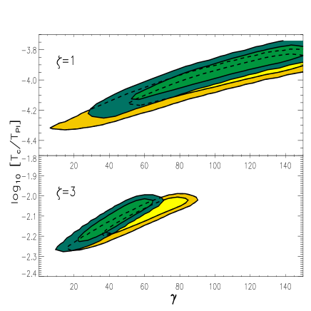
Figure 1: Marginalized confidence contours for the $\gamma$ and $\ln[T_{c}/T_{Pl}]$. The contours represent the 68% and 95% integrals. The top and bottom panels show results for $\zeta=1$ and $3$, respectively. The underlying (yellow) region is for $l_{0}=T_{c}^{-1}$ while the overlayed (green) region is for $l_{0}^{-1}=10^{11}$GeV.

$l_{0}$	$\zeta$	$\frac{T_{C}}{T_{Pl}}(\times 10^{4})$	$\gamma$	$\Delta\ln\,L$
$T_{c}^{-1}$	$\zeta=1$	$1.04^{+0.13}_{-0.14}$	$103.7^{+46.2}_{-42.4}$	$-0.75$
$T_{c}^{-1}$	$\zeta=3$	$80.3^{+6.0}_{-6.4}$	$59.9^{+8.0}_{-8.8}$	$+0.04$
$(10^{11}\mbox{ GeV})^{-1}$	$\zeta=1$	$1.18^{+0.16}_{-0.16}$	$104.2^{+45.6}_{-39.5}$	$-0.32$
$(10^{11}\mbox{ GeV})^{-1}$	$\zeta=3$	$76.4^{+6.6}_{-6.2}$	$43.0^{+6.6}_{-6.8}$	$+0.07$

Table 1: Median values for $\gamma$ and $T_{c}$. The errors are obtained from the 68% confidence integrals. The $\Delta\ln\,L$ is with respect to the best conventional power law spectrum.

It is interesting to compare our model with other alternatives. Slow-roll inflation also predicts a near scale invariant spectrum, i.e. $n_{0}=1$, with correction $n_{1}=-6\epsilon+2\eta$, in terms of slow-roll parameters $\epsilon={1\over 2}{\left(V^{\prime}/V\right)}^{2}$ and $\eta={V^{\prime\prime}/V}$, (where $V(\Phi)$ is the inflaton potential). There is also a second order logarithmic running of $n$, but for a general $V$ this is independent of $n_{1}$, since it depends on $\xi^{2}={V^{\prime}V^{\prime\prime\prime}/V^{2}}$. More generally inflation can produce any spectrum of scalar fluctuations if one carefully designs $V(\phi)$, and it’s not a falsifiable theory until we consider the tensor modes, which do impose a consistency condition. By contrast we predict a scalar “consistency condition” (19).

Our work has obvious parallels with that of rob on the Hagedorn phase. However, our phase transition is a transition in the description of space-time rather than in the matter content. This profound conceptual difference has a very practical implication: the function (8) controlling the progress of the phase transition is entirely different from that (Eqn. (12)) controlling the amplitude of the fluctuations. Thus the naturalness of scale-invariance. This is not the case with rob where both scales are controlled by $T_{c}/(T_{c}-T)$, and a degree of (debatable) fine tuning is required. It would be interesting to study how those models fare with deviations from exact scale-invariance. Our scenario can also be seen as a variant of a varying speed of light cosmology vsl0 in that in Phase I all degrees of freedom are assumed to be in causal contact and thermal equilibrium.

To conclude and summarize, we have presented a model for the emergence of classical space-time from a quantum, non-geometric pre-era informed by a version of the holographic principle. Our model develops the general idea in non-geometry in that we make particular hypotheses about the phase transition, which we labelled A) to C) above. These hypotheses could be checked in the context of different models of quantum gravity. What is remarkable is that there are specific consequences of non-perturbative quantum gravity models that may be calculable which, given our picture, map on to quantities which are measurable in the CMB. In particular the phase transition temperature is mapped to the amplitudes of fluctuations by (12), the direction of the transition-large to small scales rather than the reverse-maps to the tilt of the spectrum being red or blue, while the speed of the transition, parameterized by $\gamma$, is measurable in the tilt (17). Note that the scenario implies also the consistency condition (19) which, given $\zeta$, is a precise prediction. Alternatively, the two parameters $\gamma$ and $\zeta$ are together determined by the tilt and running of the spectrum. Our results are applicable to a large class of similar models.

We can point out that exact scale-invariance is a natural prediction of this model, without any fine tuning. This is in fact not completely ruled out by the data. However, the data presently prefers the model’s ability to produce a slightly red spectrum, with a very characteristic running, encoded in consistency condition (19). This requires large critical exponents (of order 50); whether this is reasonable or not might be investigated in explicit models of Phase I. Finally, we note that fluctuations are very nearly Gaussian pog and tensor modes are expected to be negligible in our preliminary estimates.

We thank R. Brandenberger, O. Dreyer, S. Hossenfelder, M Joyce, L. Kofman, J. Khouri, and F. Markopoulou for encouragement and discussion. CRC thanks PI and CITA for hospitality. This work was performed on the MacKenzie cluster at CITA, funded by the Canada Foundation for Innovation. Research at PI is supported in part by the Government of Canada through NSERC and by the Province of Ontario through MEDT.

References

- (1) F. Markopoulou, hep-th/0604120, in Approaches to Quantum Gravity, D. Oriti ed. CUP in press. T. Konopka, F. Markopoulou and L. Smolin, hep-th/0611197.
- (2) T. Thiemann, Class.Quant.Grav. 15 (1998) 1463.
- (3) G. ’t Hooft, gr-qc/9310006, hep-th/0003004.
- (4) L. Susskind, J. Math. Phys. 36 (1995) 6377, J. Maldacena,Adv. Theor. Math. Phys. 2 (1998) 231.
- (5) L. Smolin, hep-th/0003056; R. Bousso, Rev. Mod. Phys. 74 (2002) 825-874.
- (6) A. Liddle and D Lyth, Cosmological Inflation and Large-scale structure,CUP, Cambridge 2000.
- (7) H. Kodama and M. Sasaki, Prog. Th. Phys. 78 (1984) 1.
- (8) Spergel D., et al., 2003, Astrophys. J. Suppl., 148, 175.
- (9) A. Nayeri, R. H. Brandenberger, C. Vafa, Phys. Rev. Lett. 97: 021302, 2006; R. Brandenberger et al, hep-th/0608121 and hep-th/0608186; Biswas et al, hep-th/0610274.
- (10) J. Ambjorn, J. Jurkiewicz, R. Loll, hep-th/0604212, in Approaches to Quantum Gravity”, CUP; M. Reuter, F. Saueressig, Phys.Rev. D66 (2002) 125001.
- (11) A. Lewis, A. Challinor, A. Lasenby, Ap.J. 538,(2000), 473.
- (12) Lewis, A. & Bridle, S. 2002, Phys. Rev. D, 66, 103511
- (13) G. Hinshaw et al. astro-ph/0603451, Readhead et al. Ap.J 609 (2004) 498, Readhead et al. Science, 306, 836; Sievers et al. 2005, astro-ph/0509203; Kuo et al., astro-ph/0611198; Halverson et al. Ap. J 568 (2002) 38; S. Hanany et al. 2000, Ap.J.Lett., 545, L5; Hinshaw et al. astro-ph/0603451, Leitch et al. 2005, Ap. J., 624, 10; Dickinson, C., et al. 2004, MNRAS, 353, 732; Jones, W. C., et al. 2006, Ap. J., 647, 823; Piacentini, F., et al. 2006, Ap. J., 647, 833; Montroy, T. E., et al. 2006, Ap. J., 647, 813; Cole, S., et al. 2005, MNRAS, 362, 505; Tegmark, M., et al. 2004, Phys. Rev. D, 69, 103501.
- (14) J. Moffat, Int. J. Mod. Phys. D2 (1993) 351;A. Albrecht and J. Magueijo, Phys.Rev. D59 (1999) 043516; J. Magueijo, Rept. Prog. Phys. 66, (2003) 2025.
- (15) J. Magueijo and L. Pogosian, Phys. Rev. D67, 043518, 2003.
- (16) A. Gabrielli, M. Joyce, F. Labini, astro-ph/0110451.
- (17) D. Oaknin, hep-th/0305068; hep-th/0308078.