The variable X-ray spectrum of Markarian 766 - I.
Principal components analysis

Abstract

Aims. We analyse a long XMM-Newton spectrum of the narrow-line Seyfert 1 galaxy Mrk 766, using the marked spectral variability on timescales $>20$ ks to separate components in the X-ray spectrum.

Methods. Principal components analysis is used to identify distinct emission components in the X-ray spectrum, possible alternative physical models for those components are then compared statistically.

Results. The source spectral variability is well-explained by additive variations, with smaller extra contributions most likely arising from variable absorption. The principal varying component, eigenvector one, is found to have a steep (photon index 2.4) power-law shape, affected by a low column of ionised absorption that leads to the appearance of a soft excess. Eigenvector one varies by a factor 10 in amplitude on time-scales of days and appears to have broad ionised Fe K$\alpha$ emission associated with it: the width of the ionised line is consistent with an origin at $\sim 100$ gravitational radii. There is also a strong component of near-constant emission that dominates in the low state, whose spectrum is extremely hard above 1 keV, with a soft excess at lower energies, and with a strong edge at Fe K but remarkably little Fe K$\alpha$ emission. Although this component may be explained as relativistically-blurred reflection from the inner accretion disc, we suggest that its spectrum and lack of variability may alternatively be explained as either (i) ionised reflection from an extended region, possibly a disc wind, or (ii) a signature of absorption by a disc wind with a variable covering fraction. Absorption features in the low state may indicate the presence of an outflow.

1 Introduction

X-ray observations of many AGN show substantial flux variations, with accompanying systematic spectral variations. It is likely that the X-ray emission from AGN is composed of a number of emission components, which may or may not be interrelated, modified by the effects of absorption. The basic components of the AGN model are thought to be a continuum power-law that reflects off the surface of the accretion disk (Guilbert & Rees, 1988; Lightman & White, 1988; George & Fabian, 1991) producing an observable spectral hardening above 10 keV (Zdziarski et al., 1995; Perola et al., 2002) and strong Fe K shell emission (e.g. Tanaka et al. 1995, Nandra et al. 1997). Layers of gas are also thought to shroud the nuclear system, with a large range of ionisation-states and column densities (Creshaw, Kraemer & George, 2003).

While emission, reflection and absorption are notoriously difficult to disentangle in the mean X-ray spectra of AGN (Reeves et al., 2004; Turner et al., 2005), observed spectral changes over time can be used to attempt to decompose the emission into physically-distinct components (Taylor et al., 2003; Uttley et al., 2004; Vaughan & Fabian, 2004). By correlating the flux measured at different energies it is possible to determine the spectrum of two components: one assumed to be a constant zero-point spectrum and the other to be a component whose amplitude varies with time. The conclusion from the Vaughan & Fabian (2004) study of MCG–6-30-15 has been that there exists an underlying component of X-ray emission with a hard spectrum that appears consistent with that expected from reflection of the X-ray continuum by optically-thick gas.

Here we present results of statistical analysis of the X-ray spectral variability of Mrk 766 using principal components analysis. Mrk 766 has one of the largest integrated exposure times to date from XMM-Newton. The large amount of accumulated data combined with the high degree of flux variability exhibited in the X-ray band makes Mrk 766 an ideal target for this approach. Mrk 766 is a narrow-line Seyfert 1 at redshift $z=0.0129$ (Osterbrock & Pogge, 1985). It is known from earlier observations to have a broad component of Fe K$\alpha$ emission (Pounds et al., 2003a). Turner et al. (2006) showed that there appear to be variations in line energy consistent with an origin at around 100 gravitational radii, r_g, and, using the same data analysed in this paper, Miller et al. (2006a) showed that the ionised component of the line varies in flux with the continuum, implying an origin for the line emission consistent with that estimate. The full dataset discussed here shows that Mrk 766 exhibits a very wide range of flux levels, with marked spectral variability, and in this paper we attempt to use that information to learn more about the emission and absorption components. The variation timescales used are $>20$ ks, complementing the analysis of rapid variability by Markowitz et al. (2006). In Paper II (Turner et al., in preparation) we shall investigate direct model fits to the full Mrk 766 dataset, following up on the general behaviour discovered here.

In section 2 we summarise the method of principal components analysis and describe briefly its limitations. We have adopted a mathematical decomposition that allows us to extract component spectra with high spectral resolution despite a limit imposed by having a finite amount of data. The data used are described in section 3, and section 4 describes the principal components analysis and a statistical analysis of the results: a key point here is to decide whether or not the principal components analysis provides a good description of the source variations. Section 5 then fits some possible alternative models to the spectra of the derived components, and section 6 discusses the physical properties of the source that would be required in each model.

2 Principal Components Analysis

2.1 Introduction

A powerful method of decomposing time-variable data is to use Principal Components Analysis (hereafter PCA). PCA is widely used in multivariate analysis and has previously been used to understand the differing components of emission that comprise the optical spectra of samples of QSOs (Francis et al., 1992; Boroson & Green, 1992) and of multiple observations of individual active galaxies (Mittaz et al., 1990), and has recently been applied to the X-ray spectra of Seyfert galaxy MCG–6-30-15 by Vaughan & Fabian (2004). The mathematical model adopted is essentially the same as that assumed in the flux-flux correlation method: namely that there exist spectrally-invariant components of emission whose amplitude may vary with time. These components can then be considered as being linearly combined to produce the observed spectra. PCA allows multiple components to be detected. In principle any one multivariate dataset may be decomposed into as many components as there are measurements: as we shall describe below, a powerful advantage of using PCA is that we can test how many such components are required to explain the observed variations. The model of spectrally-invariant components may be violated in real AGN emission: an obvious example would be if there were time-varying absorption, which cannot be modelled as a series of additive components. Power-law components may also vary their spectral indices (Uttley et al., 2004). However, we may test whether such effects are present by investigating the required number of components and their shape.

To visualise the application of PCA to time-varying spectra, consider a spectrum made up of $n$ measurements, at different times, of the flux in $m$ bins of photon energy. Consider an $m$-dimensional space in which each axis is the flux in each photon energy bin: one of the measured spectra then is described by a single point in that $m$-dimensional space. The full dataset comprises a distribution of $n$ such points. If there were no variations all the points would be co-located, but if there were a single component of varying emission the distribution of points would be dispersed along a straight line passing through the origin. In general, if there were $p$ such components, the cloud of points would be confined to a $p$-dimensional surface embedded in the $m$-dimensional space. If one of those components in fact were constant, the $p$-dimensional surface could also be described in $p-1$ dimensions with a shift of the origin. One of the tasks we shall carry out is to evaluate how many dimensions are required to explain the data variations, and whether the variations may be equally well described by having one component constant.

The PCA consists of finding a coordinate rotation of the $m$-dimensional space so that one axis in the rotated system lies in the direction for which the distribution has the largest variance. This direction is known as the first principal component, or eigenvector one. The second principal component is orthogonal to the first and is the axis along which the distribution has the next largest variance, and so on. It is conventional to first shift the coordinate origin to the mean of the data distribution - this is a convenient choice as it effectively removes any constant component and allows such data to be described by $p-1$ components: the presence of a constant component can be determined by establishing whether or not the $p-1$-dimensional surface passes through the original origin. Mathematically, the principal components are the eigenvectors of the data covariance matrix, and the variances along each component are the eigenvalues. In our case of analysing spectra, each eigenvector is the spectrum of an individually varying component, and the eigenvalue measures how much variation that component is responsible for.

The principal components are orthogonal, in the sense that in the rotated coordinate system there is no covariance between the components. However, these orthogonal components need not correspond to physical components, since there need be no requirement for the true physical components to vary independently. Thus in reaching a physical interpretation of the analysis, we may need to allow that the physical components may be non-orthogonal and may be constructed out of arbitrary linear combinations of the principal components. Even in the case where the emission may be modelled as a constant zero-point spectrum plus a single varying component, the zero-point is not uniquely defined as it may lie anywhere along the vector defined by the first principal component. If we assume that both the first principal component and the zero-point spectrum are positive (corresponding to being emission components), however, then we may place limits on possible values of the zero-point spectrum. A lower bound is given by requiring that no photon energy bin should have a negative value; an upper bound is given by requiring that no observed spectrum should lie below the zero-point spectrum (as this would require a negative contribution from the varying component). Arbitrary spectra between these two extremes are not allowed: the zero-point spectrum must lie along the vector defined by the varying component. Note that this zero-point uncertainty is also present in the flux-flux correlation method described above. Fig. 1 illustrates the relationship between these various components.

One question to be investigated in the data is whether such a constant zero-point is required by the data, or whether the data are instead consistent with all spectral components being required to vary between timeslices. We shall approach this by doing two principal components analyses. In the first, we shall allow there to be a zero-point spectrum as described. In the second, we shall calculate the covariance matrix about the flux origin rather than the data mean, which in effect forces all spectral components to be variable.

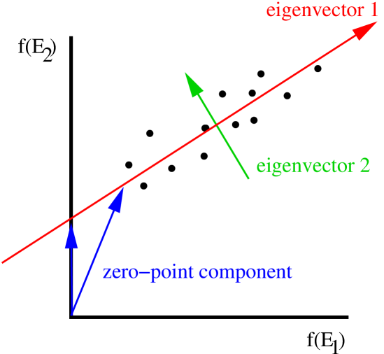
Figure 1: Schematic explanation of the relationship between PCA eigenvectors and the zero-point spectrum. The axes correspond to the flux measurements in each spectral bin (only two shown here), each point corresponds to observations in a different timeslice. The eigenvectors are orthogonal components that span the plane, the zero-point spectrum may be constructed by a linear combination of the mean spectrum and the eigenvectors, and is therefore in general neither orthogonal to the eigenvectors nor unique. The minimum and maximum possible values of the zero-point spectrum are indicated by the two arrows that start at the origin.

2.2 Singular Value Decomposition

A particular problem arises if the number of datapoints $n$ is less than the number of dimensions $m$. This situation arises in the analysis of the XMM-Newton data described below, where in order to obtain adequate signal-to-noise in each timeslice the data are limited to $n\la 60$ timeslices, but where the spectra are binned into $m\simeq 140$ energy intervals. In this case the covariance matrix is singular and the full set of eigenvectors needed to completely describe the data is not uniquely defined. However, the least significant eigenvectors simply describe shot noise in the data, whereas the most significant eigenvectors remain well-defined, being the principal axes along which the source varies. These leading eigenvectors may be extracted from the singular covariance matrix using Singular Value Decomposition (e.g. Press et al. 1992) and this is the technique used here. Hence the component spectra are reproduced at the full instrumental resolution of XMM-Newton, unlike previous analyses of X-ray data (Vaughan & Fabian, 2004).

2.3 The effects of absorption

Finally, we should return again to the question of absorption. If any component suffers time-invariant absorption, then this will not prejudice the analysis, it will simply show up as a modulation of the derived component spectra. Only in the case where the absorption varies with time will additional components apparently be created. We address this here by first considering PCA only of data in the energy range $2-10$ keV where the effects of absorption should be smallest, and then seeing the effect of extending the PCA to lower energies.

3 The data

In this paper we utilise all XMM-Newton (Jansen et al., 2001) EPIC pn (Strüder et al., 2001) data available for Mrk 766. We reanalysed the archival observations from 2000 May 20, science observation ID 0096020101 (Boller et al., 2001), and from 2001 May 20-21, science observation ID 0109141301 (Pounds et al., 2003a). We also analyse a long observation made during 2005 May 23 UT 19:21:51 - Jun 3 UT 21:27:10 over six XMM-Newton orbits, science observation IDs in the range 0304030[1-7]01. The same observations were also analysed by Miller et al. (2006a). EPIC pn data were screened in the standard way using SAS v6.5 software to select only events with patterns in the range 0 - 4. SAS v6.5 was also used to generate response matrices. We applied energy cuts to the events files to discard data below 0.2 keV and above 15.0 keV. Background filtering then removed any periods where the count rate in the background cell (a source-free region of area 3 arcmin² on the same chip as the target) exceeded 2 counts s^-1, and any periods where the background rate exceeded 5% of the source count rate. This combined filtering yielded 24 ks of ‘good’ data for 2000 May, 67 ks for 2001 May and 402 ks of ‘good’ data over a 944 ks baseline during 2005 May-June. Target photons were extracted from a circular region of $40^{\prime\prime}$ radius centred on the Mrk 766. The combination of some non-optimal MOS modes, photon pileup and inferior signal-to-noise led us to use only the pn data in this analysis.

4 Principal components analysis of Mrk 766

4.1 Generation of time-sliced spectra and the principal components

To carry out the PCA we must first divide the data into timesliced spectra that are binned in energy. The energy bins cannot be infinitesimally small because shot noise would dominate over intrinsic source variations, and the PCA would be meaningless. In order to maximise the spectral information, we choose energy bins equal in width to the half-width at half-maximum (HWHM) of the EPIC pn instrument. The HWHM varies with photon energy, so the bin widths chosen also vary with energy, from $\sim 35$ eV at $E\sim 1$ keV to $\sim 80$ eV at $E\sim 10$ keV. Hence the spectra have effectively been smoothed with a function approximately equal in width to half the energy-dependent instrumental energy resolution, and sampled at that interval. The statistical analysis of the principal components discussed in sections 4.3 & 4.5 and the model-fitting discussed in section 5 are all carried out on data analysed in this way, with spectral bins whose photon shot noise is statistically independent. To enable better visual detection of features in the spectra, the spectra displayed in sections 4.6 & 5.1 have also been smoothed with a top-hat of width two bins: in this way the spectra have been smoothed with a function close to the width of the instrumental resolution, improving the detectability of weak features but introducing greater covariance between spectral data points and degrading the resolution by a factor $\sqrt{2}$ compared with the instrumental resolution.

The signal-to-noise in each timesliced energy bin increases with the source brightness and the duration of each time slice. The time slicing must also not be chosen to be so coarse that it washes out the temporal spectrum variations. For Mrk 766 time slicing of 20 ks was found to provide a good compromise between these two criteria. Even so, the signal-to-noise at high energies, $E>7.5$ keV was found to be low, and these energy bins were grouped together until their signal-to-noise, averaged across all the observations, reached a value of 10 in each bin - degrading the spectral resolution at high energies but ensuring that the PCA remains meaningful.

The energy range chosen for the analysis initially is $2-9.8$ keV, although in section 4.5 we will extend the range to lower energies, $0.4<E<9.8$ keV. In both ranges the effective area of the EPIC pn detector exceeds $\sim 250$ cm². For brevity, in the remainder of the paper we shall refer to these energy ranges as $2-10$ and $0.4-10$ keV respectively. The spectra are analysed and displayed in units of Ef(E), where f(E) is the spectral flux density. This choice means that a power-law with photon index $\Gamma=2$ has a uniform value with energy and thus gives approximately equal weight to each photon energy bin in the spectra considered here. As the principal components are additive, each timeslice is given a weight inversely proportional to its flux so that the fractional spectral variations at low flux levels are given equal importance to those at high flux levels: otherwise the PCA results would be dominated by the high flux states, whereas we are seeking a principal components model that gives a good description of the entire dataset. With this weighting scheme, if we reconstruct a model using a subset of the principal components, we expect the data/model ratio in different timeslices to have deviations of similar amplitude irrespective of flux.

4.2 Error analysis

Errors on the resulting component spectra are obtained here by a Monte-Carlo method, in which the observed photon counts binned in energy and time are perturbed by a random amount commensurate with the photon shot noise and the PCA redone on the perturbed dataset. This process is repeated 20 times to make an estimate of the variance on the component spectra at each binned energy. Note that the errors are correlated between the various components - a deficit owing to noise on one component spectrum will be accompanied by an excess on another component at the same energy.

4.3 Results: $2-10$ keV

We first analyse spectral variations in the range $2-10$ keV, as this range should be relatively immune to the non-additive effects of any varying absorption. We first carry out the PCA assuming the existence of a constant zero-point spectrum.

We find that a reasonable description of the data can be found allowing a zero-point spectrum and a single varying component (eigenvector one). The upper panel of Fig.2 shows the amplitudes of the first two components shifted so that a spectrum with zero flux would lie at the location (0,0) on this graph. The 1st component plotted on the x-axis has a range of values 10 times larger than the second component, and, as described below, the first component accounts for $96$ percent of the variance about the mean spectrum. The extrapolation of this component does not pass through the flux origin and hence an offset zero-point spectrum is required. This is also clear if we rotate our view to look along the 1st component, and plot the scatter about that axis in terms of the next two principal components (left panel of Fig. 3): there is substantially less scatter in these two components than in the first component, and the data distribution sits away from the flux origin. Table 1 gives an indication of the number of components required to describe the data. The first column identifies the component, these being ordered by their eigenvalues. The second column gives the eigenvalue associated with each component, which is equivalent to the variance along that component. The third column gives the proportion of the total variance that is described by this component. These two measures give an indication of how much of the observed variation is explained by each component. It is clear that the first component dominates the variation.

Figure 2: Top: Amplitudes of the first two principal components for Mrk 766 assuming the existence of a constant zero-point spectrum for each individual time sliced spectrum: 1st component (x-axis) v. 2nd component (y-axis). The origin is defined as the location of a spectrum with zero flux. The 1st principal component vector is shown as the dashed line. The lower bound to this line defines the point below which the spectrum would have negative portions if composed of these two components. Bottom: As above, but with no zero-point spectrum.

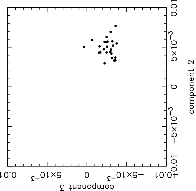
Figure 3: Left: A rotated view of the 2nd and 3rd principal components for Mrk 766, looking along the axis of the 1st principal component, and showing the offset of the distribution from the origin assuming there is a constant zero-point spectrum. Right: As above, but with no zero-point spectrum.

	with zero-point spectrum				without zero-point spectrum
#	$\lambda$		$\sigma_{f}^{2}$	$\chi^{2}$/dof	$\lambda$		$\sigma_{f}^{2}$	$\chi^{2}$/dof
	$/10^{-5}$				$/10^{-5}$
0	.		0.	4993/106	.		0.	23961/106
1	22.	5	0.956	122/105	151.	1	0.988	371/105
2	0.	14	0.0059	96/104	0.	94	0.0061	99/104
3	0.	092	0.0039	87/103	0.	11	0.0007	91/103
4	0.	082	0.0035	80/102	0.	086	0.0006	83/102
5	0.	077	0.0033	73/101	0.	077	0.0005	76/101

Table 1: The amount of spectral variation explained by the first five principal components for Mrk 766 in the energy range $2-10$ keV. Two cases are shown, one assuming there is a constant zero-point spectrum, the other without. Columns $2-4$ and $5-6$ give the eigenvalue $\lambda$, fractional variance $\sigma_{f}^{2}$, $\chi^{2}$ with numbers of degrees of freedom (dof) for each case. The fractional variances are not comparable between these two cases as the variances are defined differently.

This does not mean of course that the remaining components are not significant. We can also attempt to evaluate how well the data are described by a model comprising a zero-point spectrum plus some number of components. We have reconstructed the spectra in each 20 ks time slice from a zero-point spectrum plus the first $p$ principal components, $p=0,1,2...$, and measure the $\chi^{2}$ of the goodness-of-fit of the reconstructed to the actual spectra. The mean value of $\chi^{2}$ averaged over all time slices is given in column four of Table 1. The mean spectrum on its own results in an extremely large value of $\chi^{2}$; allowing the 1st principal component reduces the $\chi^{2}$ such that the residual fluctuations have an rms less than 10 percent larger than the photon shot noise; two variable components plus the zero-point spectrum render the PCA model an acceptable fit within each timeslice.

However, we also consider the case where no constant zero-point spectrum is allowed, with the PCA being carried out centred on the flux origin rather than the data mean. As expected from the above, a single eigenvector with no zero-point spectrum yields a rather poor fit to the data ($\chi^{2}=371$ for 105 degrees of freedom, column 7 of Table 1) despite describing 99 percent of the variance about the origin. However, two eigenvectors, with no zero-point, provide an acceptable fit, in fact almost as good as the case of a zero-point spectrum with two eigenvectors. The second eigenvector accounts of 0.6 percent of the variance and hence is substantially smaller in its variation that the first eigenvector.

We infer from this analysis that the $2-10$ keV data may be described by either: (A) two independently-varying spectral components, one of which varies substantially less than the other; or (B) a constant zero-point spectrum with one dominant varying component, plus a further varying component that could either be a true “third component” or could be an indication at a low level of some more complex variation such as would arise from variable absorption. We shall investigate this possibility further in section 4.5.

4.4 Limits on variation of the zero-point component

It is not possible from such analysis to definitively state “the zero-point component is constant” - a more meaningful statement is to place limits on the amount of variation that could arise from its variation. To make this measurement, we consider model A from above, in which two variable components are allowed, and measure the fractional variation required from the second component. We choose the energy range $2-10$ keV to minimise the effect of any variable absorption. In principle, because of the ambiguity introduced by allowing true physical components to be non-orthogonal, it is possible to find a solution in which both components have large variations. Accordingly, we choose to find the linear combination of eigenvectors that minimises the required variation in the second component. Effectively, this is measuring the scatter about a best-fit relationship between the components plotted in Fig. 2. The r.m.s. fractional variation is found to be 13 percent, with a maximum of 37 percent, so we can say that the zero-point component is consistent with being constant to about this level.

4.5 Results: 0.4-10 keV

We now extend this analysis to lower energies where we might expect any effects of variable absorption to be more noticeable. Repeating the above analysis assuming the existence of a zero-point component, indeed we find that although a small number of components give a broad description of the variations, a total of four variable components plus the zero-point spectrum are required to reduce the mean $\chi^{2}$ in each timeslice to the level expected from random noise (Table 2). However, if we take this PCA but measure the contribution to $\chi^{2}$ only in the energy range $2-10$ keV we find two components are adequate, as found in the previous section. This is partly because the shot noise errors at lower energy are substantially smaller than at high energy, and hence small fractional departures from a good fit in the low energy channels have a relatively larger effect on $\chi^{2}$, but inspection of ratios of the PCA reconstruction and the data show that the departures at lower energy are actually larger than at high energy. The natural interpretation of the need for a large number of additive components at low energies is that in fact there is variable absorption, which cannot be correctly modelled by PCA. In Paper II we measure the effects of variable absorption by fitting directly to timesliced data, a process which confirms this phenomenon.

	0.4-10 keV				2-10 keV
#	$\lambda$		$\sigma_{f}^{2}$	$\chi^{2}$/dof	$\chi^{2}$/dof
	$/10^{-5}$
0	.		0.	41250/148	4942/106
1	35.	9	0.966	745/147	121/105
2	0.	35	0.0095	349/146	104/104
3	0.	13	0.0035	165/145	90/103
4	0.	088	0.0024	148/144	81/102
5	0.	080	0.0022	133/143	75/101

Table 2: The amount of spectral variation explained by the first five principal components for Mrk 766 in the energy range $0.4-10$ keV. The left-hand set of values provide the eigenvalues $\lambda$, fractional variance $\sigma_{f}^{2}$ and $\chi^{2}$ values for the analysis over this band, the right-hand columns give the contribution to $\chi^{2}$ in just the $2-10$ keV band from this analysis.

4.6 Principal component spectra

We now turn to inspection of the spectral components that arise from the PCA. Fig. 4 shows the zero-point spectrum and first eigenvector for case B, analysed over the $0.4-10$ keV band. As described above, the spectra displayed in this section have been smoothed with a tophat function of FWHM approximately equal to the energy-dependent instrumental resolution, although all analysis is done on spectra binned only into bins of width HWHM (section 4.1). Eigenvector one is shown as the upper curve. Its amplitude varies of course, the figure shows the maximum amplitude attained by this component in the PCA. The possible lower and upper bounds on the zero-point spectrum, discussed in section 2.1, are also indicated by the pair of light-weight lines. The true zero-point spectrum must lie between these extremes, and the main zero-point spectrum shown is simply the mean of the two extremes. Note that only systematic subtraction or addition of eigenvectors is allowed.

We do not show the two eigenvectors required to describe the data for case A. As these components are forced by the PCA to be orthogonal they will not necessarily correspond to actual physical spectral components. However, candidates for such spectral components may be created from any linear combination of the two eigenvectors, and in fact it is possible to construct two components whose spectral shape is indistinguishable from the two components already shown in Fig. 4. In this description of the data, in effect, the zero-point spectrum actually shows some variation, but with variability amplitude much smaller than that of eigenvector one.

There is no guarantee that the principal component spectra produced by this mathematical decomposition will have any simple relation to actual physical emission components, yet in the spectra we can immediately see physically-recognisable features. On eigenvector one, we can see that this component is dominated by a near power-law in this energy range, but with a broad component of excess flux covering the range $6-7$ keV. Its presence on eigenvector one implies that the line emission varies with the continuum (i.e. its equivalent width is constant). Miller et al. (2006a) have identified a broad component of Fe K$\alpha$ emission from ionised Fe in the band $6.5-7$ keV that varies with the continuum on timescales $\ga 10$ ks. The PCA detection of this line on eigenvector one is in good agreement with the earlier result.

The zero-point spectrum also shows clear, physically recognisable, features. First, the overall continuum shape is extremely hard, the hard spectrum continuing up to the highest energies measured, but we can also see a strong continuum break at $\sim 7$ keV and a weak component of emission at $\sim 6.4$ keV: we identify these as the Fe bound-free edge and Fe K$\alpha$ emission from low- or medium-ionisation states of Fe. As well as the clearly-detected Fe features, there are also indications of two discrete absorption lines at energies both higher and lower than the nominal $7.14$ keV break rest energy. All these features are discussed further in sections 5 & 6.

We also see that the “soft excess” below 1 keV that is characteristic of many low-luminosity AGN is in fact present on both the variable and constant components, implying that what we see is a composite of different features. Detailed modelling of the soft excess will not be undertaken in this paper as it requires full modelling of the variable absorption.

Finally we note the effect of higher-order eigenvectors. If we suppose that there are additive approximations to a true (multiplicative) process of variable absorption, we can gauge the extent to which variable absorption might corrupt the shape of our zero-point spectrum and eigenvector one spectrum, by comparing the amplitudes. Their amplitude is such that they should have relatively little effect on physical modelling of eigenvector one. However, the effect on the zero-point spectrum could be significant, especially at energies $<2$ keV. We also note the presence of a feature in eigenvector two at energies around 7 keV: this might imply that the possible absorption lines noted above are both variable and tied to the continuum absorption variations that the rest of the eigenvector is describing.

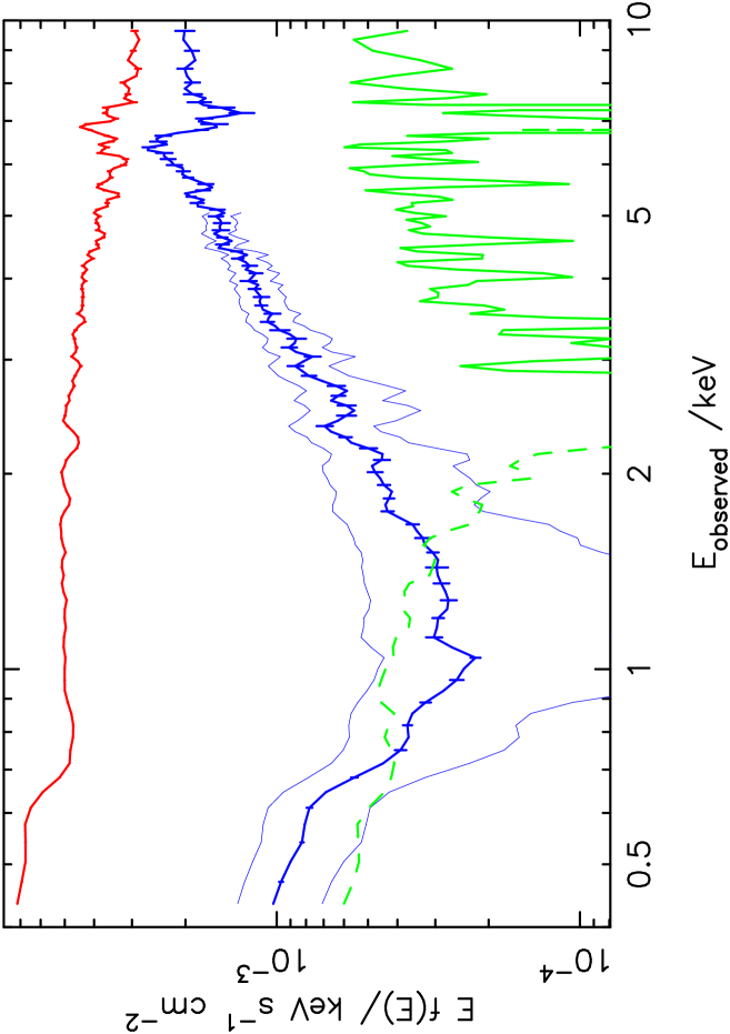
Figure 4: Principal component spectra of Mrk 766, $0.4-10$ keV. The 1st principal component is the upper spectrum, scaled to have an amplitude equal to its maximum above the mean spectrum. The possible range of the zero-point spectrum is shown by the lower set of spectra, with the upper and lower bounds discussed in the text shown as light-weight lines and the mid-point between these shown in bold. For clarity, these bounds are not plotted at energies above 5 keV where the random uncertainty becomes larger than this systematic uncertainty. The true zero-point spectrum lies between these bounds, but note that only systematic subtraction or addition of eigenvector one is allowed, these are not random noise bounds. The statistical uncertainties arising from shot noise are determined as described in section 4.2 and are shown by the error bars on each spectrum (the errors on eigenvector one are very small). The second principal component is also shown. Errors on this component are large but are omitted for clarity. At low energies the component is negative: the dashed portion of the curve shows the absolute value of the component.

5 Physical interpretation of the principal components

5.1 Comparison with data

The above statistical analysis demonstrates that the data may be described by a small number of variable components, but there is no guarantee that these mathematical decompositions correspond to physical components. In the following sections we shall investigate a range of physical models that may correspond to the principal components, but first we should investigate whether the principal components actually yield a good description of the data. Fig. 5 compares the PCA reconstruction with the actual data. To reduce the effect of photon shot noise in this comparison, the data have been averaged into five flux states, defined in equal logarithmic intervals of flux. The left-hand figures show the $2-10$ keV analysis of section 4.3: in this band the spectral variability is greatest at the lowest energies and the flux integrated in the $2-5$ keV band was used to define each flux state. The right-hand figures show the $0.4-10$ keV analysis of section 4.5; here the variability is greatest in the $1-2$ keV band and this was used to define the flux states. In both cases the PCA reconstruction was made from the zero-point spectrum plus the first two eigenvectors.

It can be seen that the PCA models provide good agreement with the variations present in the data. In the $2-10$ keV range the fit is almost everywhere better than about 5 percent, apart from the extreme high and low energy limits. In the $0.4-10$ keV range there is evidence for systematic departures at the level of 10 percent, especially at low energy, as expected from the previous statistical analysis. Overall, we conclude that the dominant spectral variability is indeed well described by the simple additive model, although a detailed description of the data will need to allow variable absorption. The zero-point spectrum and eigenvector one are sufficiently well-defined that we shall now proceed to see if they can be fit by physical models of X-ray emitting regions in AGN.

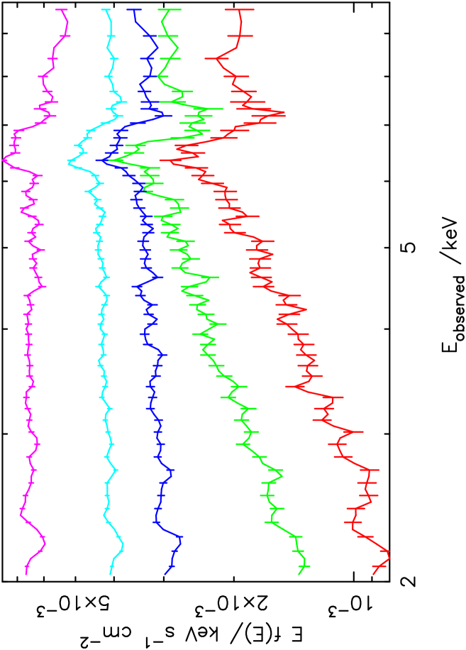
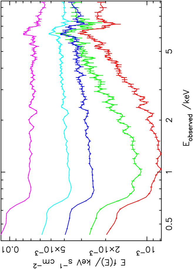
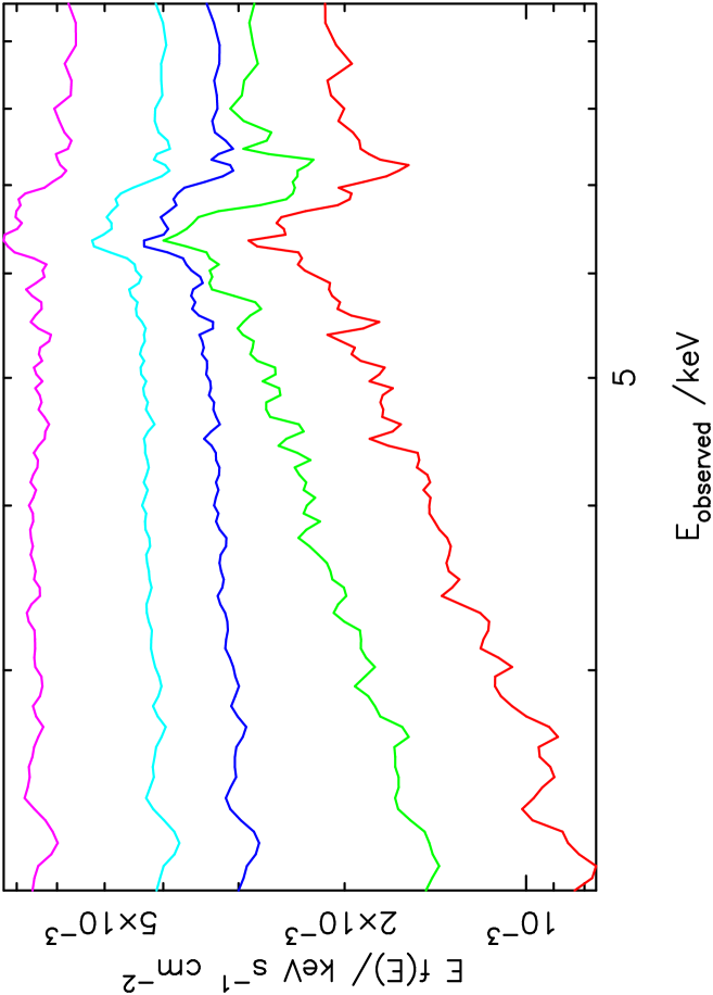
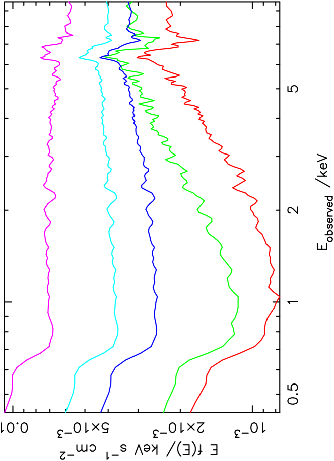
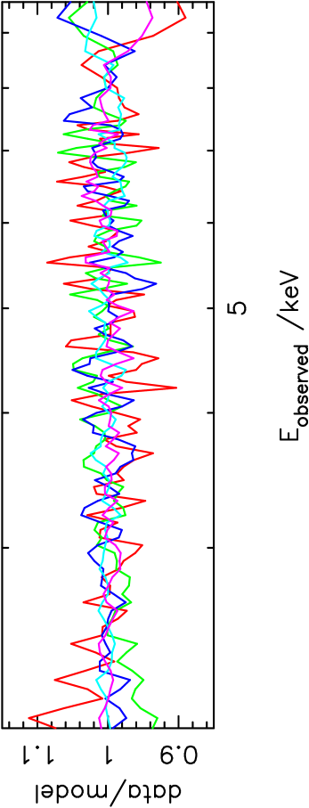
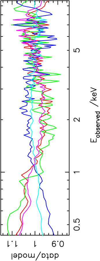
Figure 5: Data used for the PCA, averaged into five flux states compared with the PCA reconstruction. Left side: $2-10$ keV analysis, flux states defined in the range $2-5$ keV, right side: $0.4-10$ keV analysis, flux states defined in the range $1-2$ keV. Top: data averaged into the five flux states; centre: PCA reconstruction, using the zero-point spectrum plus the first two eigenvectors; bottom: ratio of data and PCA model (note the expanded y-axis scale).

5.2 Model-fitting to Eigenvector one

We now fit physical models to the principal component spectra using the fitting software xspec (Arnaud, 1996). Because the PCA is a decomposition of the data, the component spectra that are produced are convolved with the instrumental response function. Hence these components may be treated as data for the purposes of fitting. The actual instrument response of XMM-Newton varies with time, and the PCA is based on observations obtained over the period 2000-2005. We use the instrument response functions from 2001, when the source was in its high state. Uncertainty in the true response function causes some systematic uncertainty in the spectral fitting, which may be largest for steep spectrum sources such as Mrk 766. Comparison of contemporary MOS and pn observations of Mrk 766 indicates this uncertainty could be as large as 5 percent. There are also systematic uncertainties arising in the generation of the PCA component spectra: physical spectra may comprise any linear combination of the eigenvectors, and when fitting over the full energy range $0.4-10$ keV we have seen that a large number of components are required to adequately describe the data. Overall then, we should not expect a perfect fit between physical models and the component spectra. In fitting to eigenvector one we allow a 3 percent systematic error to be added in quadrature with the random error when calculating $\chi^{2}$, although even this is likely to be an underestimate of the true systematic error in some regions of the spectrum. One such region is the energy range $2.0-2.7$ keV, which is just above the energy of a sharp drop in the instrumental effective area. Convolution of this sharp edge with the energy response function results in residual ripples propagating into the principal components, visible in Figs 4-5. We exclude this spectral range when fitting eigenvector one.

The model we fit to eigenvector one comprises two components. The overall spectrum is assumed to be a power-law affected by warm absorption: an absorption grid was created from xstar (Kallman et al., 2004) and its column and ionisation parameter were allowed to be free parameters. In the absorption models generated, the input source was assumed to be a power-law of photon index 2.4. The best-fit absorber parameter values were $N_{H}=2.7\times 10^{21}$ cm^-2 and $\log\xi=1$ (hereafter $\xi$ will be in units of  erg cm s^-1). The ionised line reflection component was provided by a grid of “reflion” models (Ross & Fabian, 2005), with power-law index of the illuminating radiation tied to that of the main power-law component, and with the reflection ionisation as a free parameter. The reflection spectrum was convolved with a Laor et al. (1991) model using the xspec routine “kdblur”. Additional warm xstar absorption was also allowed on the reflection component, with best-fit values $N_{H}=3.3\times 10^{22}$ cm^-2 and $\log\xi=1$. This simple fit provides a good description of the overall spectral shape, with a value of $\chi^{2}=142$ for 124 degrees of freedom, assuming a 3 percent systematic error. The model agrees with the component spectrum everywhere better than 10 percent. However, the fit is poor is around the broad Fe line, and the line shape is not well reproduced. In fact the data are better fit by a simpler model comprising only a warm-absorbed power-law plus a line at 6.7 keV blurred by the same Laor model as above: i.e. without including the reflected continuum and Compton broadening that we expect to be associated with ionised reflection. The best-fit value of power-law index in steep, $\Gamma=2.38\pm.01$ (statistical error) $\pm.05$ (estimated systematic error obtained from fitting to higher energies alone). Additional narrow components of “emission” at rest energies of 6.97 and 7.3 keV, not blurred by an accretion disc, improve the fit further: we discuss the interpretation of these components below. The fit is shown in Fig. 6: $\chi^{2}$ has now improved to 116 with 124 degrees of freedom. The range of accretion disc radii responsible for the ionised line is not well-determined: the best-fit value for the inner radius of the emission assuming a disk emissivity power-law index of 3 and an inclination angle of $30^{\circ}$ is $r_{\rm in}\simeq 100$r_g, but no useful upper or lower limit on this value is defined by the fit to the line profile, largely as a result of allowing the additional narrow line components in the fit.

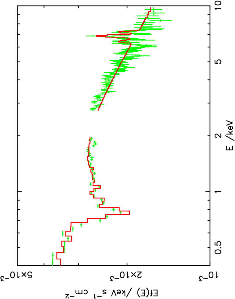
Figure 6: The fit to eigenvector one, with a model of an absorbed power-law and some simple line components (see text). The solid curve shows the model, points with errors the “unfolded” spectrum. The spectrum in this plot is normalised to the value given by the eigenvalue, i.e. to the eigenvector’s rms amplitude.

The two additional “emission” components occur at the energies of likely absorption lines identifiable in the zero-point spectrum, at rest energies 6.97 and 7.3 keV, which are discussed below. It seems likely that the components visible on eigenvector one are in fact indicative of those absorption lines disappearing as the source brightens, rather than being a genuine emission component. Overall, we conclude that the principal varying component, eigenvector one, is likely to comprise a variable power-law component and an associated broad reflected ionised Fe line to be discussed further in section 6, although the actual lineshape may be contaminated by the effects of varying absorption. The worse fit of the reflion model implies that the reflected continuum expected to be associated with the ionised line has however not yet been clearly detected through its spectral shape.

5.3 The zero-point spectrum

An extremely hard spectrum and strong Fe K edge as seen in the zero-point spectrum might arise from either a component of “reflected” emission from neutral or moderate-ionisation optically-thick gas (George & Fabian, 1991; Magdziarz & Zdziarski, 1995; Ross & Fabian, 2005), or from ionised absorption of the continuum source. If reflection arises from the inner regions of an accretion disc it may also be relativistically blurred. In this section we attempt to fit a number of possible physical models to the zero-point spectrum. From the analysis in section 4 it seems likely that this component is significantly affected by variable absorption below $\sim 1-2$ keV, and hence in this paper we concentrate on fitting to the energy range $1-10$ keV. In fact, the most important diagnostics for interpreting the physical origin of this emission are the Fe K emission line and absorption edge. Two features are particularly noticeable. First, the absorption edge, although having a large decrement, is soft and appears blurred or absorbed to energies lower than the canonical (rest) energy of 7.14 keV expected from neutral material (Kallman et al., 2004). Second, the equivalent width of neutral 6.4 keV Fe K$\alpha$ is much weaker than expected if this component is identified with pure reflection from low ionisation material: the observed equivalent width is $\sim 50$ eV compared with the expected value $\sim 1$ keV (George & Fabian, 1991).

There are a number of possible explanations for the low equivalent width and apparently soft edge, and we discuss some of these in turn by fitting an appropriate model to the zero-point spectrum. We noted in section 2.1 that this component is not uniquely defined: the actual zero-point spectrum could have any amount of eigenvector one added to it in order to produce the set of possible zero-point curves shown in Fig. 4. We deal with this in the following manner. We choose to fit to the zero-point spectrum deduced from the $0.4-9.8$ keV PCA that is the maximum of the allowed extremes shown in Fig. 4. Then, when fitting physical models to this spectrum, we allow also a variable amount of eigenvector one to be included in the fit. This process thus exactly mimics the systematic uncertainty in the definition of the zero-point spectrum. The only complication is that eigenvector one is defined as data, convolved with the instrumental response, so in order to correctly include this in the fitting we allow an arbitrary amplitude of the model fit to eigenvector one, rather than eigenvector one itself. We find that no component of systematic error is required in fitting the zero-point spectrum in the $1-10$ keV range. We also do not exclude the range $2.0-2.7$ keV as we did for eigenvector one: the larger random uncertainties on the zero-point spectrum mean that the systematic errors on the component spectrum in this energy range do not significantly affect the values of $\chi^{2}$ obtained.

5.3.1 Absorption lines in the zero-point spectrum

Inspection of Fig. 5 indicates the presence of two absorption features, possibly lines, at observed energies about 6.9 and 7.2 keV, most prominently in the lowest flux states. These features also appear in the PCA zero-point spectrum, as shown in Fig. 4. Whether these features are actually absorption lines does depend on the model adopted for the K-edge and continuum, so their statistical significance is assessed in each of the specific models discussed below. They appear primarily on the zero-point component spectrum because their absorbed flux is approximately constant: absorption lines of constant equivalent width would appear on eigenvector one. The most natural interpretation of their appearance on the zero-point component is that these are indicative of an absorbing region that is physically localised to the region represented by the zero-point component. Having said that, the positive features that appear at these energies in eigenvector one, and also in eigenvector two, may indicate a more complex variability behaviour for these absorption lines.

If the lines are real, their identification is ambiguous. The feature observed at 6.9 keV could be 6.97 keV Fe XXVI Ly$\alpha$ in the rest-frame of the source, or it could be Fe K$\alpha$ absorption with some outflow velocity ($\sim 13,000$ km s^-1 for 6.7 keV K$\alpha$ or $\sim 22,500$ km s^-1 for 6.5 keV K$\alpha$). The feature at 7.2 keV could be 7.3 keV Fe XIX K$\beta$ in the source rest-frame, although in this case we would expect to see a broad complex of Fe absorption in this region of the spectrum (Kallman et al., 2004). Alternatively, it could be blueshifted absorption: 6.97 keV Fe XXVI Ly$\alpha$ at $\sim 13,000$ km s^-1 or Fe K$\alpha$ absorption ($\sim 26,500$ km s^-1 for 6.7 keV K$\alpha$ or $\sim 37,000$ km s^-1 for 6.5 keV K$\alpha$). Any of these cases are indicative of a high column density of ionised ($\log\xi>2$) gas. The $13,000$ km s^-1 solution is interesting as it might imply a common origin for both lines. Further discussion of the identification of these features and their variability is postponed to Paper II: in the following sections we allow for their possible presence by including Gaussian absorption lines of variable amplitude at these two energies.

5.3.2 Model components for the zero-point spectrum

In the following we present a number of alternative model fits to the zero-point spectrum. Each model has the same general structure, although the detailed components vary.

First, we assume that the low-column, low-ionisation absorption that was identified in the fit to eigenvector one is also an absorption layer in front of the zero-point spectrum. The parameters of this layer are frozen at the values found above. Then, the zero-point spectrum is allowed to comprise three components: (i) some variable amount of eigenvector one, as discussed above; (ii) a component of ionised reflection or absorption (depending on the model below) whose incident illumination is a power-law of the same slope as eigenvector one, the slope being a fixed parameter; and (iii) a component of neutral reflection with an unresolved 6.4 keV Fe emission line of equivalent width 900 eV with respect to the reflected continuum, a typical value expected for a steep-spectrum reflector (George & Fabian, 1991). Component (iii) is modelled within xspec using the “pexrav” function (Magdziarz & Zdziarski, 1995). We also allow an additional component of ionised absorption to be in front of component (ii), the ionised reflection/absorption: this might arise if the reflecting surface has its own atmosphere, for example.

Although fairly complex, this is probably a minimal set of components for a physical model of the emitting regions, and the quality of the data and principal component spectra that we have extracted do demand fitted models of this complexity. Variants on the above general model are easily envisaged (in particular, the choice of which absorbing layers cover which emission regions) but in the fitting below we keep the same general structure for all models in order to allow fair comparison between them.

Finally, we note again the important caveat that we are here not fitting directly to data but to the PCA zero-point spectrum. Depending on the interpretation of eigenvector two, in terms of models A or B of section 4.3, the zero-point spectrum below 2 keV may either be significantly affected by variable absorption (model B) or not (model A). Thus too much reliance should not be placed on the parameter values that are found when fitting to the zero-point spectrum: the important point is to find out whether physical models can be found which may in principle explain the existence of the zero-point spectral component, and if so what range of models may suffice.

5.3.3 Relativistically-blurred disc reflection

A similar component to Mrk 766’s zero-point spectrum arises also in MCG–6-30-15 (Vaughan & Fabian, 2004), and in that case the spectral shape is thought to arise from relativistic blurring of reflection from an accretion disc. We investigate whether such an explanation is viable in Mrk 766, first by fitting to the zero-point spectrum in this section, and then discussing the required geometry of such a model in section 6.

To create a model of blurred reflection, we take the ionised reflection “reflion” model of Ross & Fabian (2005) and blur it with a Laor et al. (1991) convolution model, provided in xspec by the “kdblur” function: a layer of ionised absorption is also allowed as described above. This then is used as component (ii) in fitting, together with eigenvector one and the neutral reflection components. An important feature in the ionised reflection component spectrum is the depth of the Fe K edge, which is determined by both the abundance of Fe and the geometry of the reflection. The latter is not a variable in the reflection model, but we can allow the Fe abundance to vary. For consistency we scale the pexrav model and its associated Fe K$\alpha$ line to the same abundance value. The best-fit value was found to be 0.35 times solar: this model provides a good fit to the spectrum over the range $1-10$ keV (Fig. 7) with $\chi^{2}=96$ for 122 degrees of freedom, with 10 free parameters. We note here that this fit is much better than expected given the assumed size of error bars. We believe this is because of neglect of covariance between spectrum points, so that in effect the true number of degrees of freedom is smaller than assumed. Nonetheless, the fit is clearly good. Increasing the Fe abundance to 0.5 increases $\chi^{2}$ to a value 103, forcing Fe abundance to have the solar value results in $\chi^{2}=162$. The maximum departure between the $1-10$ keV spectrum and the best-fitting model is $\sim 15$ percent. The best-fit reflion ionisation parameter is $\xi\simeq 700$ erg cm s^-1with an absorbing layer of column $N_{H}=3\times 10^{22}$ cm^-2 and $\log\xi\simeq-1$. The relativistic blurring has a major effect in this model, the inner radius of the emission having a best-fit value equal to the minimum allowed value in the model of r${}_{\rm in}=1.235$r_g. The unblurred neutral reflection is an important component in allowing the blurred model to fit the data: without it $\chi^{2}$ increases to a value 480, even allowing the remaining parameters to vary. The flux in the $1-10$ keV band provided by the blurred component is $3.3\times 10^{-12}$ erg cm^-2 s^-1 and by the neutral component is $0.5\times 10^{-12}$ erg cm^-2 s^-1. The two absorption lines discussed in section 5.3.1 also appear to be significant in this model: $\Delta\chi^{2}$ is found to be 40, 44 or 74 in the absence of the 6.9 keV, 7.2 keV or both absorption lines, respectively, so in the fitted model a substantial part of the softening of the Fe K edge is caused by the presence of absorption.

Is relativistic blurring required? Increasing r_in even to a value 6r_g increases $\chi^{2}$ by 23, so it seems that, in the reflion model fitted here, relativistic blurring is strongly favoured. It is possible to obtain a reasonable (but not good) fit of such an optically-thick ionised-reflection model to the zero-point spectrum without requiring relativistic blurring, provided that the iron abundance is allowed to be low: a model comprising neutral reflection plus absorbed “reflion” reflection with ionisation parameter $\ga 1000$ erg cm s^-1  both with Fe abundance 0.13 times solar and covered by an ionised absorber can fit the component spectrum with $\chi^{2}=160$ with 9 free parameters and 123 degrees of freedom in the $1-10$ keV range. In fact, we expect the equivalent width of the emission lines to be geometry dependent in optically-thick reflection: the apparently low Fe abundance may instead be a signature of a different geometry from that assumed in the Ross & Fabian (2005) model. However, in the following sections we consider whether more extreme variations from the assumptions of the reflion model may provide alternative explanations of the zero-point component without requiring relativistic blurring.

5.3.4 Non-relativistically blurred reflection models

In this section we investigate alternative reflection scenarios which might be able to explain the spectral shape without requiring relativistic blurring. In this case the reflecting material could be placed at larger distances from the central illuminating source, allowing the lack of variability to be explained as arising from the light travel-time delay. The critical question becomes, “can the strong Fe K-edge but weak Fe K$\alpha$ emission line arise naturally in reflection models?”. The low equivalent width of 6.4 keV Fe K$\alpha$ makes it infeasible that the zero-point spectrum may be fit by a standard low-ionisation reflection model. It seems likely therefore that, regardless of whether it is relativistically blurred or not, if there is a substantial component of reflection then it is from Fe-ionised material.

There are three ways in which ionised reflection might be able to generate a spectrum close to that observed. The first is to suppose that the reflector is a high column, close to being optically-thick, of very highly ionised gas that reflects radiation from the central X-ray source through Compton scattering off free electrons. In order to obtain a reflected intensity close to that observed the scattering medium would need to cover a substantial fraction of the source: the evidence in favour of such a model is discussed in section 6. The observed spectral shape would be produced by a high column of some separate intervening absorption of intermediate ionisation. The existence of an outer layer of lower ionisation material might be a natural expectation for a region of gas photoionised by a central source. We therefore model component (ii) in our generic scheme as being a component of absorbed scattered radiation whose shape is parameterised as an absorbed component of eigenvector one with absorbing column and ionisation parameter being free parameters. We compared absorber models with two values of Fe abundance, solar and 0.67 times solar: the latter provides a significantly better fit (note that we also had to allow low Fe abundance in the blurred reflection model). In principle we could have allowed Fe abundance to be a free parameter in the fitting, but it was somewhat prohibitive to generate a wide range of xstar absorption models: in practice we find that the choice of 0.67 already provides an excellent fit to the data, so investigation of a wider range of abundance was not justified. The best fit values for the absorber were found to be $\log\xi=3.0$, $N_{H}=4\times 10^{23}$ cm^-2: For consistency with the other models discussed here, this component is also covered by a low-ionisation absorbing layer which has best-fit values $N_{H}=5\times 10^{22}$ cm^-2, $\log\xi\simeq 0$. The fit of this model, shown in Fig. 7, is actually better than in the case of blurred ionised reflection: $\chi^{2}=83$ with 9 free parameters and 123 degrees of freedom (although we should decrease the number of free parameters by one to account for the freedom of choosing a non-solar abundance). Again, the pair of absorption lines are required in this model, they play a significant role in defining the shape of the edge around 7 keV. The best-fit model does predict some amount of 6.5 keV Fe K$\alpha$ seen in absorption: if we require a value for the ionisation parameter $\log\xi<2.5$ in order to avoid any $6.5$ keV absorption, we find $\chi^{2}$ to be slightly higher, with a value $94$ for 124 degrees of freedom, but still a very good fit to the data.

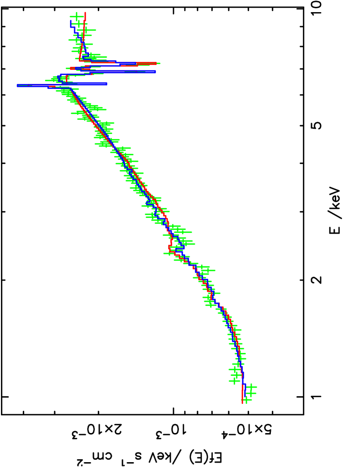
Figure 7: Fits to the zero-point spectrum showing the relativistically-blurred model (red curve, lowest of the two models at 10 keV) and the non-blurred ionised-opacity model (blue curve) with the unfolded data points, with errors.

A second way of obtaining the observed spectrum could be from a reflector of intermediate ionisation, Fe ionised in the range Fe XVIII-XXIV, such that the K$\alpha$ line can be resonantly scattered and destroyed by the Auger effect (Ross et al. 1996; Matt et al. 1996; Zycki & Czerny 1994, see also Liedahl & Torres 2005). Resonant Auger destruction arises in the “reflion” models of Ross & Fabian (2005) and has already been suggested for a model incorporating a reflection component in Mrk 766 by Matt et al. (2000). However, we have already seen in section 5.3.3 that the optically-thick reflion models do not provide the best fit to the spectrum without relativistic blurring. The reason is that in the reflion model with $\xi\sim 300$ erg cm s^-1the opacity of the gas within the reflecting region falls sufficiently low that strong emission lines from lower ionisation material, particularly 6.4 keV Fe K$\alpha$, are produced.

As an example of a model that might avoid this problem, consider a region of reflecting gas illuminated from within by the central X-ray source of the AGN, such as a wind or atmosphere above the accretion disc being illuminated by a central X-ray source. The distant observer would have both a direct view of the central source and a view of reflected radiation from the wind or atmosphere. If the density within the scattering region falls off with radius, perhaps as fast as $r^{-2}$, the ionisation state of the gas could be high throughout, diminished only by the opacity of the gas (as in the plane-parallel reflecting slab). However, the column of gas may be only just Compton-thick, perhaps $N_{H}\la 10^{24}$ cm^-2, so that the gas opacity does not become too high: if the source covering fraction is high, a scattered intensity comparable to that observed in Mrk 766 could be produced without having a high equivalent width in either 6.4 keV or 6.5 keV Fe K$\alpha$ line emission.

To correctly model the expected spectrum from such a scattering region would require a radiative transfer code similar to that of Ross & Fabian (2005), incorporating the effects of resonant scattering and Auger destruction, constructed with a relevant geometry, far beyond the scope of this paper. However, if the range of ionisation parameter within the gas is small we can approximate the resulting spectrum by considering the effect of absorption on an incident spectrum, and we might expect that again model component (ii) may have a spectrum whose shape is parameterised as an absorbed power-law. This is approximately true in the reflion optically-thick slab model: in this $\xi$ range, the effect of Compton energy redistribution on the spectrum shape is small, and the continuum shape in the 1-10 keV range is dominated by the gas opacity within the reflecting zone. In this case, we would require the range of ionisation to allow resonant Auger destruction, i.e. $2.5\la\log\xi\la 3.5$ for photon spectral index $\Gamma=2.4$. One sophistication that would differentiate the ionised reflection component from a simple absorbing model is that we assume the high-ionisation zone is responsible for scattering or reflecting the incident radiation: in this case both the expected 6.5 keV Fe K$\alpha$ line and the continuum are assumed isotropically scattered, and hence no 6.5 keV absorption line should appear in its spectrum. This would not be the case if we were viewing a background radiation source in transmission through the ionised gas, when we would expect Fe K$\alpha$ to be seen in absorption. If we artificially remove 6.5 keV Fe K$\alpha$ absorption by allowing a cancelling emission line in the model fit, a slightly higher ionisation parameter is favoured, $\log\xi\simeq 3.1$, with an improved $\chi^{2}=78$ with 122 degrees of freedom. We emphasise that a proper evaluation of this suggestion does require construction of a reflection model incorporating the full range of opacity expected, given the chosen geometry.

Finally, the observed Fe K$\alpha$ emission may be further suppressed geometrically in models of reflection from extended regions: because the Fe K$\alpha$ line opacity is much higher than the continuum opacity, the observed Fe K$\alpha$ photons are effectively seen from a relatively thin outer scattering layer: if the region is arranged to have greater surface area oriented away from the observer, substantially reduced observed line emission may result (Ferland et al., 1992).

5.4 Absorption-only models

Given the success of the absorption fits in the preceding section, we consider whether in fact models comprising only absorption, and no reflection, may explain the data. In order to explain the time-variation in spectral shape, either the opacity must vary, or the emitting source must be only partially covered by an absorber whose covering fraction varies. Crucially, any such model must satisfy the requirement that the resulting spectral variation yields the appearance of arising from additive components, in order to yield the observed PCA results. It thus seems highly unlikely that in fact the opacity could vary in just such a way to mimic the effect of two primary additive components in the data, as displayed in Fig. 2, throughout a range of a factor 10 in flux at $\sim 2$ keV. We do not consider such variable-opacity models further here.

The partial covering model seems more viable however: in this case the observed spectrum again comprises two additive components, and because the true components may be formed from any linear addition of the components deduced in section 4 such a model must fit the data equally as well as the reflection models considered above. In essence, the time-dependent source spectrum would be a linear combination of an absorbed component that dominates in the low state and an unabsorbed component that dominates in the high state, with a smooth progression in the relative contribution of each between these states. The only distinguishing feature might be that in this case we might expect to see Fe K$\alpha$ absorption from the ionised absorber that is required to fit the spectral shape; no absorption in the rest-frame is detected, although one of the lines at 6.9 or 7.2 keV could be blueshifted Fe K$\alpha$.

Pounds et al. (2004) have also suggested a similar scenario for the Seyfert 1 AGN 1H $0419-577$, and argue that its spectral variability may be explained either as a component of extremely blurred inner-disc emission or as absorption partially covering the continuum source.

The physical constraints on such a model are interesting: in this picture the factor ten variations in source flux are caused by the covering fraction variations. The source flux varies extremely rapidly, with a break in the power spectrum at a frequency $\sim 5\times 10^{-4}$ Hz (Vaughan & Fabian, 2003; Markowitz et al., 2006). This is the orbital timescale at $\sim 10$r_g for black hole mass $4\times 10^{6}$ M_⊙. However, the analysis presented here has only considered spectral variations on timescales as short as 20 ks, so we might suppose that some other process produces the extremely rapid variability, but that the partial covering varies on periods $\sim 40$ ks. This timescale corresponds to the orbital timescale at $\sim 70$ r_g. Either the absorption would arise from this scale, in order to produce the observed time variability, or the emitter is both extended and inhomogeneous on this scale, producing variability by moving behind a patchy absorber.

An intriguing example of an absorber model has been suggested by Done et al. (2006), who propose that an outflowing disk wind should produce an edge-like P-Cygni profile: they show that such a model fits the spectral shape of 1H $0707-495$. Interestingly, the model can produce both an edge at about the energy of the atomic transition considered (Done et al. 2006 assumed 6.95 keV) and also absorption at higher energies. It may be that the overall shape of the edge and 7.2 keV (in the observed frame) absorption seen in Mrk 766 may also be explained by such a model. If the observed-frame 6.9 keV absorption is real, however, this might need an additional non-outflowing absorbing layer. Models corresponding to this proposal are discussed by Done et al. (2006) but are not yet generally available, so fitting of such a model is postponed to future work. Observationally, we might expect absorption and reflection models to have different signatures at very hard energies near the “Compton hump”, and this might be testable with Suzaku observations, although Done et al. (2006) point out that high columns of absorbing material would in any case lead to significant reflection also.

6 Discussion

6.1 The principal varying component

It seems very likely that the primary variable component in Mrk 766 has the form of an absorbed power-law, with accompanying ionised reflection that varies with the continuum. This conclusion is in direct agreement with the conclusions of Miller et al. (2006a) who measured the correlation between ionised line emission and continuum variations in the same dataset. The index of the power-law is consistent with being unchanging over the four year period, and the goodness-of-fit of a small number of PCA components implies that substantial variation in spectral index (see e.g. Poutanen 2001) does not seem to be occurring in Mrk 766. In the analysis presented here, measurement of the ionised line profile appears to be contaminated by the effect of variable absorption, but the line width does appear consistent with an origin at about 100 r_g, consistent with the analysis of the 2001 data by Turner et al. (2006) who found evidence for periodic Doppler shift of ionised emission from a radius $r\sim 100$r_g (assuming a disc inclination $\sim 30^{\circ}$). Thus the three analyses yield a consistent location for the line emission.

6.2 The zero-point spectrum

The physical interpretation of the zero-point spectrum is however more ambiguous, and no definite conclusion can yet be reached on its origin. It may be that the blurred K-absorption edge and weak 6.4 keV line are a result of relativistic blurring with an inner radius for the emission $<6$r_g. However, this leaves a number of puzzles. This component appears constant to within 37 percent, with an rms fractional variation of 13 percent, over the period 2000-2005, despite variation in the illuminating continuum of a factor 10. A similar dilemma has been found for MCG–6-30-15, which has many similarities with Mrk 766 (Miniutti et al., 2003; Vaughan & Fabian, 2004). To explain this behaviour whilst retaining the inner-disc hypothesis, two possible explanations have been proposed.

The first invokes gravitational bending of light from an illuminating hotspot around the black hole, in such a way that the continuum from the hotspot appears to vary while the reflected emission from the disc remains approximately constant (Miniutti et al., 2003; Miniutti & Fabian, 2004). Given the result of Miller et al. (2006a), confirmed by the PCA, the reflecting accretion disc at $\sim 100$r_g also needs to see the same apparent continuum variation as the distant observer, because the reflected emission varies closely with the continuum. It may be difficult to create a geometry that would allow this, especially if the phenomenon of a constant reflected component is a general feature seen in many AGN.

Merloni et al. (2006) propose an alternative explanation for the lack of variation of inner-disc emission. They predict the emission expected from an unstable radiation-pressure-dominated accretion disc, which has both density and heating inhomogeneities, and conclude that variability of the reflected emission could be suppressed in this model. It is not yet clear however whether the variation over long timescales would be as small as observed in Mrk 766, nor whether the variability could be reinstated at 100r_g. The role of the accretion disc in suppressing variation in reflection has also been discussed by Nayakshin & Kazanas (2002), who find that reflection variations may be suppressed on timescales comparable to the disc dynamical timescale. However, if the reflected emission originates at only a few gravitational radii, the dynamical timescale is expected to be much shorter than sampled by our analysis. In this case we would still expect to see longer-term variations in the reflected emission which are not observed, so this effect seems unlikely to explain the apparent near-constancy of the zero-point component on timescales $>20$ ks.

An alternative interpretation of the lack of variability in this component is dilution of variations by light travel-time, with emission coming from regions significantly more distant than the inner accretion disc. However, we then need to explain the lack of Fe K$\alpha$ emission. In the model fitting, we considered two possible scenarios for a “distant reflector” hypothesis. In the first, the reflector was assumed to be a high column of highly-ionised gas covering a large fraction of the source, with a separate absorbing layer being responsible for the hard spectrum observed. In the second, the hard spectrum could arise from the opacity of the reflecting material itself, rather than being an absorbing layer that is separate from the reflecting medium. In the second case Fe K$\alpha$ emission would need to be suppressed either geometrically or by resonant Auger destruction.

The existence of such gas may be expected from models of the central regions, and King & Pounds (2003) have proposed that optically-thick winds should be expected from high Eddington-ratio AGN. Ionised gas of density $\sim 10^{7}$ cm^-3 would be Compton thick if extended over a region larger than $\sim 10^{17}$ cm: such a region would have a light-travel-time radius of about one month, sufficient to explain the lack of variability in the reflected spectrum. In the model of a disc wind associated with a $10^{8}$ M_⊙ black hole by Proga & Kallman (2004), $\sim 80$ percent of the source is covered by a column of $N_{H}\sim 5\times 10^{23}$ cm^-2 gas with $\log\xi>4$ out to the largest radius simulated in their model of $\sim 5\times 10^{16}$ cm, and this region would not need to be much larger in order to achieve a Compton scattering depth about unity. There is also observational evidence for such gas: the existence of significant columns of ionised absorption has long been recognised (e.g. Kraemer et al. 2005; Turner et al. 2005 and references therein). In our X-ray observations of Mrk 766 the most plausible identifications of the twin absorption lines observed at $6.9$ and $7.2$ keV require a high column ($\ga 10^{23}$ cm^-2, dependent on line identification and velocity dispersion of the gas) of high ionisation (possibly as high as $\log\xi\sim 5$ depending on line identification) gas. Confirmation of this zone should be a high priority for future spectroscopic observations. High-column outflowing winds have also been proposed to explain observed absorption features in other AGN (Reeves et al., 2003; Pounds et al., 2003b). There is also evidence from optical polarisation studies of AGN that a high column of ionised material is responsible for scattering above the accretion disc at radii comparable to the broad-line region: Smith et al. (2005) infer a column $\sim 4\times 10^{23}$ cm^-2 between radii $1.5$ and $2.4\times 10^{17}$ cm, extrapolation to smaller radii would imply the existence of an absorbing layer that is Compton-thick to radiation from the central source, albeit with unknown covering fraction. We have therefore suggested that reflection from an extended atmosphere or wind may provide a spectrum similar to that deduced from the PCA. Higher resolution spectroscopy of the region around 7 keV should again allow the possible models to be distinguished.

6.3 The absorption lines

Given the limited resolution of XMM-Newton and the complexity of the spectra around the Fe K-edge, it is difficult to be certain that the absorption features at 6.9 and 7.2 keV are discrete lines. Both models considered here do require them however. The lines are interesting in themselves, as they may be indicative of high-velocity, high-ionisation outflow, as mentioned above. Both lines may be produced by gas with $\log\xi\sim 4$ with outflow velocity $13,000$ km s^-1: interestingly gas can acquire such radial velocities in the disc wind model of Proga & Kallman (2004) discussed above. High velocity H- and He-like Fe absorption also appears in the model of Sim (2005), which aims to explain the apparent high outflow velocity in PG $1211+143$. High ionisation outflows have also been detected in Galactic X-ray sources (e.g. Kotani et al. 2000, Miller et al. 2006b). In Mrk 766, higher resolution data would help clarify the nature of these features, although it does appear that they are only strong in the low state. It is possible that these absorption features are symptoms of a much more dramatic absorption signature, in which the entire Fe K edge is produced by P-Cygni-like absorption from a disc wind, as suggested by Done et al. (2006). In this case the wind would need to have a variable covering fraction in order to reproduce the observed spectral variability. The variability timescales suggest a wind origin again $\sim 100$r_g.

7 Conclusions

Our main conclusions may be summarised as follows.

• Principal components analysis reveals that a relatively simple additive model can explain the complex spectral variability of Mrk 766: namely that there is a variable component dominated by a soft power-law component, of constant power-law index, together with relatively non-variable component(s) constant to $\sim 40$ percent.

• A variable ionised Fe emission line is detected on the principal varying component, eigenvector one, that is probably high-ionisation reflection from the inner accretion disc, consistent with the analysis of Miller et al. (2006a) of the same dataset. The best-fit models indicate an origin at $\sim 100$r_g for the ionised Fe emission assuming a disc inclination angle $\sim 30^{\circ}$.

• The relatively unchanging zero-point component has a hard spectrum with a pronounced Fe K edge but only weak Fe K$\alpha$ emission, whose spectrum seems to require ionised reflection or absorption. The Fe K edge appears soft and is likely affected either by a combination of relativistic blurring and absorption, or by absorption alone.

• If the zero-point component originates as reflection from the inner accretion disc, the detection of correlated variation of the ionised Fe K$\alpha$ emission line with the continuum implies that the accretion disc at $\sim 100$r_g has the same view of the central source as a distant observer, whereas the inner disc sees a much reduced variation in illumination.

• An alternative explanation for the lack of variation is that the emission arises from a reflecting region that has a physically large size ($\ga 1$ light-week). The lack of Fe K$\alpha$ emission may be achieved by scattering and absorption of nuclear emission either by an extended zone of ionised gas with $\log\xi\sim 2-3$ or by a very highly ionised zone ($\log\xi>4$) accompanied by some further absorption. It is possible that this component could be reflection from a hot dense wind or atmosphere such as that modelled by Proga & Kallman (2004). Further modelling of such reflecting regions is needed to test this explanation.

• There appear to be discrete absorption lines at observed energies 6.9 and 7.2 keV. The identification of the lines is not secure, but they may arise in an outflow of velocity $\sim 13,000$ km s^-1. In the blurred reflection explanation, these lines cannot arise from the same region as the reflection, as they would be blurred themselves, so their appearance in the low state of Mrk 766 would need to be explained as a dependence of opacity on the flux state of the source.

• The results from the PCA could alternatively be explained by models of ionised absorption in which the fraction of the source covered is variable. The variability timescale would imply an origin at $\sim 100$ r_g for the absorbing material. It is possible that the disc wind model proposed by Done et al. (2006) may be able to explain both the principal component spectra and the spectral variability, if the wind is clumpy.