astro-ph/yymmnnn
Large Non-Gaussianities in Single Field Inflation
Xingang Chen1, Richard Easther2 and Eugene A. Lim2
1 Newman Laboratory, Cornell University, Ithaca, NY 14853
2 Department of Physics, Yale University, New Haven, CT 06511
Abstract
We compute the 3-point correlation function for a general model of inflation driven by a single, minimally coupled scalar field. Our approach is based on the numerical evaluation of both the perturbation equations and the integrals which contribute to the 3-point function. Consequently, we can analyze models where the potential has a “feature”, in the vicinity of which the slow roll parameters may take on large, transient values. This introduces both scale and shape dependent non-Gaussianities into the primordial perturbations. As an example of our methodology, we examine the “step” potentials which have been invoked to improve the fit to the glitch in the for , present in both the one and three year WMAP data sets. We show that for the typical parameter values, the non-Gaussianities associated with the step are far larger than those in standard slow roll inflation, and may even be within reach of a next generation CMB experiment such as Planck. More generally, we use this example to explain that while adding features to potential can improve the fit to the 2-point function, these are generically associated with a greatly enhanced signal at the 3-point level. Moreover, this 3-point signal will have a very nontrivial shape and scale dependence, which is correlated with the form of the 2-point function, and may thus lead to a consistency check on models of inflation with non-smooth potentials.
1 Introduction
The Cosmic Microwave Background is a treasure trove of information about the primordial universe. An exciting set of current and future experiments [1, 2, 3] will yield an even richer data set, allowing us to make precise tests of inflationary models via their predictions for the form of the primordial perturbations. Typically, these predictions are expressed in terms of the power spectrum, or 2-point function. For a general set of initial inhomogeneities, further information about the perturbations might be gleaned from their higher order correlation functions. If the perturbations are exactly Gaussian, then the N-point functions vanish exactly when is odd, and is fully specified in terms of the 2-point function for even .
All inflationary models predict some level of non-Gaussianity. Moreover, non-linear corrections will generate non-Gaussianities in the CMB even if the primordial spectrum is purely Gaussian [4]. Thus any observed non-Gaussianities will be a combination of the primordial non-Gaussianity laid down during inflation, and that arising from weak second-order couplings between modes. A rough measure of the non-Gaussianities is provided by the parameter ,
| (1.1) |
where is the gravitational potential which sources the temperature anisotropies in the CMB [5]. Generically, second order couplings between modes yield , while it has been shown in great detail that for standard single field slow roll inflation, , where is the usual slow roll parameter [6]. The two contributions are cumulative, and the primordial 3-point function is thus swamped by the evolutionary contribution. Moreover, cosmic variance ensures that even a perfect CMB dataset will not allow a conclusive detection of the 3-point function if is of order unity. In addition, the presence of foreground contamination [2, 7] further complicates observational efforts. Current estimates suggest that Planck can achieve a limit of [8]. In this paper paper we will show that this may permit the detection of interesting features in the 3-point statistics for some classes of scale-dependent inflationary models.
The 3-point correlation function is a separate and independent statistic. Therefore it potentially discriminates between models of inflation with degenerate power spectra. More optimistically, if the amplitude of the 3-point function is large enough for us to map its dependence on both the scale and shape of the momenta triangle, this will be an enormous boon to early universe cosmology, since the 3-point function encodes information in both these properties. However, to realize this possibility, we need to compute the 3-point correlation function for a given inflationary model, and compare these predictions to data. Here we show how to compute the 3-point function for a general model of inflation driven by a single, minimally coupled scalar field. Crucially, we do not assume slow roll, and our methodology applies to both simple models with smooth potentials, and more complicated scenarios where the potential has an isolated “feature”. Since the 3-point function can have both shape and scale dependence, our calculations will underscore the limitations of a single scalar statistic such as . Our analysis is purely theoretical, and we do not compare our computed 3-point function to data, but this issue is being actively addressed by others [9].
As cosmological data improves, we will frequently be faced with the problem of interpreting “glitches” in the observed power spectra, and determining whether these represent genuine departures from some concordance cosmology. For instance, the derived from the temperature anisotropies in both the 1 Year and 3 Year WMAP datasets show a noticeable departure from the best fit LCDM spectra around , and the fit can be improved by adding a small “step” to the inflationary potential. The best-fit parameters for this step were extracted from the 1 Year data set in [10], and from the 3 Year dataset in [11], and the two analyses find broadly similar values. Of course, any proposal that adds free parameters to the inflationary potential is likely to produce a better fit to data. The question then turns to whether this improvement is good enough to justify the additional parameters. If we focus solely on the 2-point function, this question is addressed via the resulting change in the per degree of freedom, or by Bayesian evidence. However, we will see that a potential with a sharp, localized feature induces a massive enhancement of the primordial 3-point function, relative to our expectations from slow-roll. This enhancement is sufficiently dramatic to boost the non-Gaussianities to the point where they may be detected experimentally. Consequently, this provides a stringent check on any proposal for a nontrivial inflationary potential, since the specific form of the non-Gaussianities will be heavily correlated with the 2-point function. Such correlations will also extend to higher order statistics such as the trispectrum and beyond, though we do not consider them here [12, 13, 14, 15, 16, 17, 18].
In models with a non-trivial potentials, an accurate computation of the power spectrum must be performed numerically. We begin our examination of the 3-point function by reproducing existing semi-analytical results that assume slow roll. We then analyze a specific model where the inflaton potential has a small, sharp “step” [19] to illustrate our methodology in a non-trivial setting. Since this model has already been used to improve the fit between LCDM cosmology and the observed power spectrum, we can take the best-fit parameter values for this step and compute the resulting 3-point function. Interestingly, although such a feature only causes a small correction in the 2-point correlation function , it amplifies the non-Gaussianity by a factor around 1000. Roughly speaking111As we will discuss later, is not a good statistic for such non-trivial non-Gaussianities, although it remains useful as a rough guide to the amplitude of the 3-point function., is boosted from to , making the non-Gaussianity a potentially useful constraint. The leading term in the cubic Lagrangian responsible for this boost differs from those used in the previous calculations in Ref. [6, 20, 21].
The distinctive feature of this non-Gaussianity is its dependence on the scale of the momenta triangle [22]. Firstly, it has a characteristic “ringing” behavior; as we will see, a suitably defined generalization of oscillates between positive and negative values. Secondly, the impact on the 3-point function is localized around the wavenumbers that are most affected by any feature, and dies away over several e-folds. These features distinguish a step model from other single field theories with large non-Gaussianities, such as DBI inflation [23, 24] or k-inflation models [25], where the non-Gaussianities are present at all scales and the running is very slow [26, 22, 21, 27, 28].
This paper is divided into the following sections. Section 2 details the step potential model that we are considering; we lay out our conventions in this section. Section 3 details the analytic forms of the 3-pt correlation functions, which we will proceed to integrate numerically in Section 4. We discuss our results in Section 5 and conclude in Section 6.
2 Slow roll model with a feature
For single field inflation driven by a minimally coupled scalar, the action is
| (2.2) |
where the potential is designed such that the inflaton field is slowly rolling for long enough to drive inflation. We define the slow roll parameters by222Note these are related to the potential slow roll parameters via , , by , .
| (2.3) | |||||
| (2.4) |
For the quadratic potential, , . Assuming transplanckian field values, or , both slow roll parameters and their higher derivative cousins are sub-unity.
We add a step into the slow roll potential, with the form proposed by [19]
| (2.5) |
where the step is at , with size and gradient respectively. While the presence of the step at just the “right” place would require a tuning, one can imagine potentials with many steps, so that the odds are high that at least one of them would fall inside the range of relevant to the cosmological perturbations.
As discussed in [30, 19] this step induces an oscillatory ringing in the power spectrum. When the inflaton rolls through the step, it undergoes a strong momentary acceleration. In realistic models the step is typically less than 1% of the overall height of the potential. In this case, at all times, and . On the other hand, and its higher derivatives can grow dramatically as the inflaton crosses the step, often to the point where they exceed unity, as shown in Fig. (1).
We begin with an order of magnitude estimate of the values of the slow roll parameters. The step has a depth and a width (setting ). When the inflaton falls down the step, of the potential energy is converted to kinetic energy, resulting in an increase in on the order of , within a time interval . Using these quantities, we can estimate
| (2.6) |
and
| (2.7) | |||||
These values have the same order of magnitude as the peaks obtained numerically in Fig. 1.
After this acceleration, the inflaton is damped by the friction term in
| (2.8) |
and relaxes to the attractor solution. This relaxation time is determined by the first two terms in Eq. (2.8), and is of order . This corresponds to the decay width of the peaks in Fig. 1. It is easy to see that and during the relaxation are of order and , respectively. Our numerical results were obtained with , – the central values of the step corresponding to the low- glitch analyzed by Covi et al. [11]. Thus , and get , consistent with Fig. 1. Note that is chosen to be around 1 in the plot, is the conformal time, and prime is the derivative with respect to .
The non-linear couplings of the perturbations are proportional to powers of the slow roll parameters which characterize the background evolution, even when the slow roll parameters are large. Consequently, a deviation from slow roll results in a large mixing (“interaction”) of modes, and large non-Gaussianities. The amplification of the non-Gaussianity relative to a smooth potential is roughly characterized by . From our previous discussion we know that the during relaxation after traversing the feature is of order . During acceleration this quantity will depend on the firm of the feature, and is greater than unity for the step potential. Thus any sharp feature will greatly boost the non-Gaussianity.


3 3-point correlation functions
In this section, we sketch out the derivation of the 3-point correlation function, following [6, 20, 21], writing in terms of integrals over conformal time , with the integrand being a finite expansion in slow roll parameters. Although we work with the step potential, the analysis is applicable to a generic feature. We begin by perturbing the fields in the ADM metric [31]
| (3.9) |
using the comoving gauge [32, 6]
| (3.10) |
where and are Lagrangian multipliers, and is the scalar perturbation. Note that in this gauge vanishes. The power spectrum is given by the 2-point correlation function of the curvature perturbation
| (3.11) | |||||
where is the power spectrum.
The 3-point correlation function is substantially more complicated. As non-Gaussianities arise from departures from nonlinear couplings, we must compute the action (2.2) to cubic order in the perturbation:
| (3.12) | |||||
where
| (3.13) | |||||
| (3.14) | |||||
| (3.15) |
Here is the inverse Laplacian and is the variation of the quadratic action with respect to the perturbation . The cubic action (3.12) is exact for arbitrary and . Note that the highest power of slow-roll parameters which appears is of , when we recall that contains a multiplicative factor of . The fact that the series expansion in slow-roll parameters is finite is important since, although remains small in the presence of a feature, and may become large. The last term in (3.12) can be absorbed by a field redefinition of ,
| (3.16) |
After this redefinition, the interaction Hamiltonian in conformal time is
| (3.17) | |||||
It is more convenient to work in Fourier space, so
| (3.18) |
The field redefinition equation (3.16) introduces some extra terms in the 3-point correlation function,
| (3.19) | |||||
where denotes the Fourier transform of – note that this is not the square of . In (3.19), the slow roll parameters are evaluated at the end of inflation. Although we can no longer perturbatively expand in terms of if is large, the terms that we neglected are of higher order in . Since , we can neglect these unless becomes ridiculously large, which it never does in any case of interest to us. We have only considered the first term in (3.15), since all other terms involve at least one derivative of , and vanish when evaluated outside the horizon.
The 3-point correlation function at some time after horizon exit is then the vacuum expectation value of the three point function in the interaction vacuum
| (3.20) |
Before we proceed, let us pause and point out a subtlety hidden inside equation (3.20): the 3-point on the left hand side is evaluated with the interaction vacuum while the the right hand side is evaluated at the “true” vacuum. The interaction Hamiltonian evolves the true vacuum to the interaction vacuum at the time we evaluate the 3-point function. Neglecting this will lead to errors as first pointed out by Maldacena [6, 33, 34].
The three terms in the second line of (3.17) are of higher order in slow-roll parameters, and were properly neglected in Refs. [6, 20, 21], which assume that and are always small. In our calculation, the terms are small, but the term may be large and in fact dominant. the step.
We now decompose into its Fourier modes and quantize it by writing
| (3.21) |
with associated operators and mode functions
| (3.22) |
where and satisfy the commutation relation . The “true” vacuum is annihilated by the lowering operator . The power spectrum is then
| (3.23) |
with is evaluated after each mode crosses the horizon.
Meanwhile is the solution of the linear equation of motion of the quadratic action,
| (3.24) |
where we have used the definitions
| (3.25) |
Our choice of vacuum implies that the initial condition for the mode function is given by the Bunch-Davies vacuum
| (3.26) |
where we have neglected an irrelevant phase, since (3.24) is rotationally invariant.
To compute the 3-point correlation function, one simply substitutes these solutions into equation (3.17), and integrates the mode functions from through to the end of inflation. This integral can be done semi-analytically for simple models, provided the slow roll parameters are small and relatively constant. Any departures from this serene picture will render the semi-analytic approach intractable – including the step potential we consider here.
Inspecting equations (3.17) and (3.20) and recalling that , it is clear that the 3-point correlation function consists of a sum of integrals of the form
| (3.27) |
| (3.28) |
where is either or . In a single field model after Hubble crossing as it freezes out, while oscillates rapidly at early times, so its contribution to the integral tends to cancel. Thus the integral is dominated by the range of during which the modes leave the horizon.
Now let us consider the potential (2.5). We expect , making (3.27) negligible. However, and can clearly be very large as changes rapidly over a very short time. This flagrant violation of slow roll means that we expect a large contribution from the term in the integral, of the order , where is the acceleration time for the inflaton by the feature. From the qualitative estimation in Sec. 2, we know this is . The best parameters from Covi et al. for a step that matches the low- glitch seen in current CMB data are and [11]. Thus we expect a boost in the 3-point statistic of at scales affected by the step. Given that the baseline 3-point function is proportional to , we see that this pushes the expected value up to from .
We now focus on the term, and relegate the discussion of the subleading terms to an appendix (where a field redefinition term is also subleading since the effect of the feature dies away towards the boundary). So our leading term is
where the “two perm” stands for two other terms that are symmetric under permutations of the indices 1, 2 and 3, where 1, 2, 3 are shorthand for , and .
4 Numerical Method
The equations of motion for the background fields and the perturbations are
| (4.29) | |||||
| (4.30) | |||||
| (4.31) | |||||
| (4.32) |
where is our time parameter. We choose initial conditions and units for such that the step occurs around , and the mode with comoving wavenumber crosses the horizon at the same point. The initial conditions of the perturbations are given by (3.26).
We need to evaluate (3) and equations (A.47) to (A). They all have the form (3.27) and (3.28). At early times the integrand is highly oscillatory and the net contribution per period is thus very small. However the early time limit of the integral must be handled with care, since a sharp cutoff imposed by a finite initial time will introduce a spurious contribution of into the result.
Analytically, the standard procedure is to Wick rotate the integral slightly into the imaginary plane [6, 20, 21] in order to eliminate the oscillatory terms. Unfortunately, it is not straightforward to implement this approach numerically. Instead we introduce a “damping” factor into the integrand
| (4.33) |
and similarly for the term. This is approximately equivalent to rotating the contour integral from the real axis slightly into the imaginary plane . The relative error introduced by this numerical procedure can be estimated by taking the difference between the integration over and and is thus . If we ensure
| (4.34) | |||||
| (4.35) |
then this contribution is negligible, recalling that .
We can adjust both and . Choosing an appropriate combination will damp out the oscillatory contributions at early times while having no effect on the integrand during Hubble crossing, which provides the dominant contribution to the 3-point function. We tested this scheme against the known analytical results for 3-point functions, which we match to within a few percent. However, and are set by hand in our code, so while this approach is suitable for an initial survey, we are developing a more flexible scheme333Since finishing this paper, we have developed a more robust numerical methods which regulates the integral at early times without using a damping factor [35]. The regularization is prone to suppressing the 3-point function since pushing to large negative values make the numerical integrations very time consuming. In practice the results shown here for the step potential may be lower than their exact values, with a greater suppression at larger values of .. As an aside, the imaginary component of the integral goes to infinity, scaling as . However, as long as we stop the integration a few efolds after horizon crossing, the integration is stable.
5 Results and Discussion
5.1 Shape and Scale
Every 3-point correlation function has two main attributes: shape and scale. Unlike previous treatments, we cannot assume that the 3-point function is scale invariant. Before we compare the analytical and numerical results, let us define a more useful parameter than the rather unwieldy raw 3-point function,
| (5.36) |
We have factored out the product , since during inflation and there are 6 factors of in the 3-point function. The function depends on the details of the integrals listed in Sect. 3 and is some constant that we will come back to later. If the slow roll parameters stay small and constant we can factor the power spectrum out of [6, 20, 21]
| (5.37) |
where is a quantity of and the convention here follows Ref. [21]. In terms of ,
| (5.38) |
Since the power spectrum is statistically isotropic [36], we assume that this is also true in the bispectrum and impose rotational symmetry so that, combined with the conserved momentum constraint, the 3-point correlation function depends only on the amplitudes of the ’s.
Recall the definition of , equation (1.1), which is often used when computing the non-Gaussianities in the CMB sky [37, 38, 1, 8]. Current constraints on , from 3 years of WMAP data are [39]
| (5.39) |
As pointed out in [29], this ansatz assumes that the 3-point correlation function has the following local form
| (5.40) |
or, in terms of
| (5.41) |
In other words, the constraint (5.39) is applicable only if the primordial non-Gaussianities have the local form (5.40).
Since equation (1.1) does not contain an explicit scale, this form is scale-invariant (neglecting the correction terms)
| (5.42) |
Note that there is a small violation of scale-invariance in the 3-point correlation function stemming from the power spectrum term which we have ignored in the proceeding argument. In fact, equation (5.40) itself hides a further ambiguity: at what value of are we evaluating the power spectrum? This omission is justified if we assume that the power spectrum is almost scale-invariant, which is true for most “standard” slow roll single scalar field models. However, for the step potential we are considering, the power spectrum itself undergoes drastic oscillations of . We will come back to this point later.
5.2 Quadratic () inflation
Following [6], we can write down the explicit form of
| (5.44) |
where terms include . Comparing this to the local form equation (5.41) we can see that for the equilateral case, where the second equality comes from the fact that for the potential (5.43). In the other extreme of the squeezed triangle case, . This result was first derived by Maldacena, who pointed out that for single field slow roll inflationary models, and is thus unobservable. We compared our results to equation (5.44), and as Figure 2 shows, our code is accurate to within a few percent, which is within the error expected from the analytical estimate itself.

Since the potential has no features, the 3-point correlation function is essentially “scale independent”. By this, we mean that triangles which exhibit scaling symmetry posses identical values for their 3-point functions.
5.3 Step potential
Confident that our code is robust, we now compute the 3-point correlation functions for the step potential (2.5). We focus on the best fit model of Covi et al. [11] for a step which affects modes at large angular scales, namely where . We choose the same inflaton mass used with the model, so that we can compare the results.

Consider the power spectrum, Figure (3). As first described in [19], the violation of slow roll induces a temporary growing/decaying behavior in the evolution of the modes before horizon crossing, resulting in a “ringing” of the power spectrum. Thus we cannot simply factor out the power spectrum from as we have done in equation (5.37); doing so will introduce spurious contributions to any statistic that we might obtain.444For example, dividing it by [40, 41] will entangle the ringing in the power spectrum with the ringing in the bispectrum. The 3-pt correlation function is, in principle, a completely independent statistic from the 2-pt correlation function. In our definition, we make it clear that the only content of the division by is simply to state that the 3-pt amplitude is roughly the product of 2-pt amplitude. In the future, we envisage that the 3-pt will be part of the set of cosmological parameter space that we can constrain from observations of the CMB and large scale structure, and this definition completely disentangle the 2-pt from the 3-pt and thus avoid any unphysical cross-correlations between the two statistics. On the other hand, we expect the 3-point correlation to be of order , so if we set in equation (5.36) where (i.e. the observed value of the power spectrum), then the dimensionless quantity
| (5.45) |
is what we want to plot. This quantity has the great advantage that the strong running from the scaling of the 3-point correlation function (see for example equation (5.42)) is factored out, so we are left with the scaling that is generated by from the non-linear evolution of the modes.
Consider the equilateral case, Figure (4). Analogously to the power spectrum, the presence of the step induces a ringing of the equilateral bispectrum. The ringing frequency in the 3-point function is roughly 1.5 times that in power spectrum, due to the presence of three factors of in the integrand instead of two.

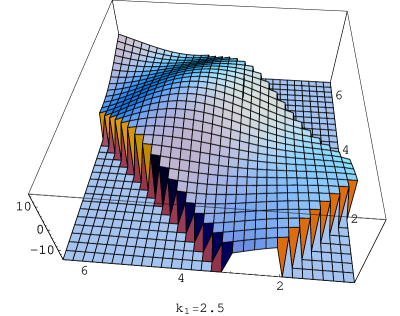
The plots in Figures 5 illustrate the complicated landscape of the non-Gaussianities. Compared to the amplitude of the model, the non-Gaussianities are magnified several hundredfold and can be larger for other viable step parameters (Figure 7), since we are taking the mid-point values from Covi et al.. As we explained in Sec. 3, the dominant contribution to the non-Gaussianities comes from the term (Figure 1). As we estimated, is of order since the contribution from the term is . This is confirmed by our numerical results; the shape of the non-gaussianity remains constant but its amplitude is rescaled as we vary and together (Figure (7)).
In Figure 6, we plot the integrand with respect to for the modes which cross the Hubble horizon around the step. We have suppressed the early time oscillations via our “damping trick” in order to isolate the actual contribution to the integral. The step also occurs around this time. Comparing this with the plot Figure (1), we see that the oscillatory nature of modulates the single hump of , yielding complicated structures. Depending on the combined phases of the modes, the modulation can be both constructive and destructive, leading to the “ringing” of the primordial bispectrum. The non-linear interactions between the modes have become dominant due to the large coupling term around crossing, mixing up the perturbations in non-trivial manner and generating large departures from Gaussianity. This is in contrast to the ringing of the power spectrum which is caused by the change in the effective mass of the modes as they cross the horizon.
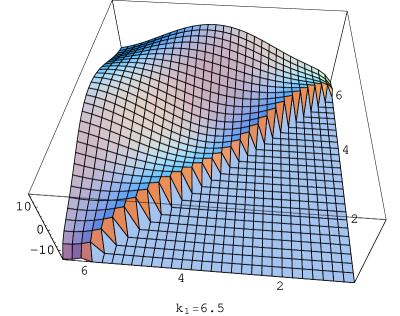
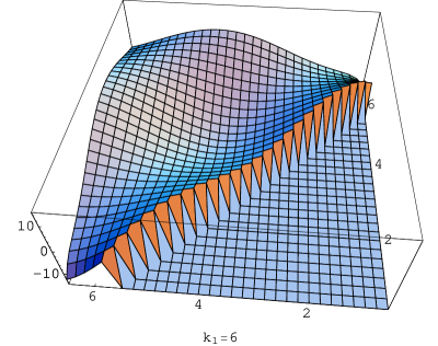
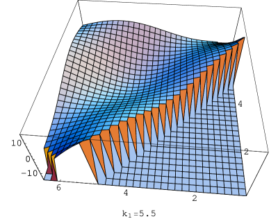
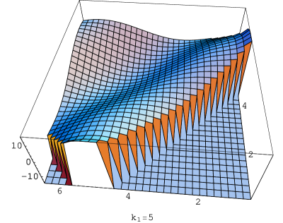
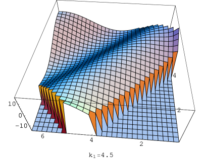
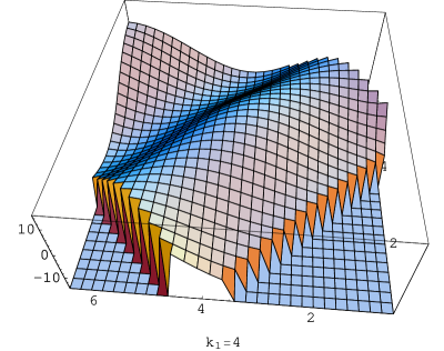
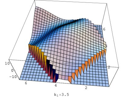
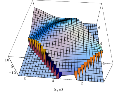


To bound this specific non-Gaussian signal with current WMAP data, we would have to redo the full sky analysis using the data for our complicated scale and shape dependent predictions of the bispectrum. This is not a trivial task and requires new methods to be developed before we can approach the problem. A brute force computation of the likelihood is computationally daunting since the bispectrum here is clearly unfactorizable into a product of separate integrals over the ’s555A recent paper [44] has begun to address this important question.. However, we can make some guesses. We have previously alluded to the fact that the statistic (5.45) is similar to . By comparing equation (5.41) to equation (5.45), we see that
| (5.46) |
Since the factor is roughly of then which is within sights of the next generation CMB experiments [8]. However, in our case only a subset of all possible triangles we could draw on the sky have a large 3-point function, which increases the risk that cosmic variance will swamp any signal. On the other hand, we have a specific template for the 3-point function, which can then be cross-correlated with the 2-point function associated with any putative step.
6 Conclusion
While simple models of slow roll inflation do not exhibit observable non-Gaussianities, the space of models of inflation that can produce a power spectrum which fits the CMB data is infinite. To discriminate between these degenerate models, some other independent statistic derived from the CMB must be used and the bispectrum is becoming the most promising candidate for this role. Unlike the power spectrum, the computation of the bispectrum for a given inflationary model is a messy affair. In this paper, we have developed a robust numerical code which can compute the 3-point correlation function for a non-slow roll single field model.
Using this method, we numerically integrated the 3-point correlation functions for a class of inflationary models where slow roll is violated for a brief moment. We show that the addition of this step breaks the scale invariance of the bispectrum in a non-trivial way, leading to large non-Gaussianities. This numerical technique can be extended to solve more complicated problems such as multifield models of inflation [42, 43] and to compute higher statistics such as the trispectrum [16].
Mirroring the behavior of the power spectrum, a temporary violation of slow roll introduces a ringing into the bispectrum, resulting in a structure much like the transient vibrations of a rug being beaten. These large non-Gaussianities are generated when the non-linear coupling between the modes, , becomes temporarily large during this period of non-slow roll behavior. In order to check whether we can constrain such models with data, a full sky analysis must be undertaken with either current or future data, a task which is beyond the scope of this paper. However, we argue that at least for the models considered in this paper, the non-Gaussianities may be large enough to be within reach of the Planck satellite.
In the near future we can expect even better quality CMB data to become available, opening up the possibility of cross-correlating higher order statistics such as the bispectrum with the power spectrum. This should provide a powerful consistency check on any models of inflation with a sharp feature in the potential, even if this improves the fit to the 2-point function. Consequently, we have laid the groundwork for an analog of the “consistency relationship” of simple models of slow roll inflation, where the amplitude and slope of the scalar and tensor spectra are expressed as functions of just three independent parameters - the observed amplitude of the scalar spectrum, and the first two slow roll parameters, and . In this case considered here, the parameters that describe any step or other near-discontinuity would fix both the 2- and 3-point functions, yielding a consistency test for a very broad class of inflationary models. In practice we could fit separately to the 2- and 3-point functions and then check that the results matched. Alternatively, one could simultaneously include information from both the power spectrum and bispectrum into the cosmological parameter estimation process. In this case, we could fit directly to the parameters , and (along with the “average” slow roll parameters), generalizing the approach of [45, 46]. Finally, if it ever becomes possible to determine the 3-point function from observations of large scale structure, this information would further tighten the constraints on models where slow roll is briefly violated.
7 Acknowledgments
We thank Wayne Hu, Hiranya Peiris, Kendrick Smith, Henry Tye and an anonymous referee for a number of useful discussions. XC thanks the physics department of Yale university and KITP for their hospitality. XC is supported in part by the National Science Foundation under grant PHY-0355005. RE and EAL are supported in part by the United States Department of Energy, grant DE-FG02-92ER-40704.
Appendix A Other terms
In Section 3, we have given the expressions for the leading non-Gaussianity in the case when is large but remains small. In this appendix, we give the expressions for the subleading terms for this case from the Hamiltonian (3.17).
The subleading contributions come from the first line of (3.17). Contribution from term:
| (A.47) |
Contribution from term:
| (A.48) |
Contribution from term:
The redefinition (3.15) contributes
| (A.49) |
Note that in Ref. [6, 20, 21], where sharp features are absent, these four terms give leading contributions to non-Gaussianities.
The last two terms in (3.17) are further suppressed by , but for completeness we list their contribution in the following. Contribution from term:
Contribution from term:
References
- [1] D. N. Spergel et al., “Wilkinson Microwave Anisotropy Probe (WMAP) three year results: Implications for cosmology,” arXiv:astro-ph/0603449.
- [2] R. Scoccimarro, E. Sefusatti and M. Zaldarriaga, Phys. Rev. D 69, 103513 (2004) [arXiv:astro-ph/0312286].
- [3] M. Liguori, F. K. Hansen, E. Komatsu, S. Matarrese and A. Riotto, Phys. Rev. D 73 (2006) 043505 [arXiv:astro-ph/0509098].
- [4] T. Pyne and S. M. Carroll, “Higher-Order Gravitational Perturbations of the Cosmic Microwave Phys. Rev. D 53, 2920 (1996) [arXiv:astro-ph/9510041].
- [5] E. Komatsu and D. N. Spergel, Phys. Rev. D 63, 063002 (2001) [arXiv:astro-ph/0005036].
- [6] J. M. Maldacena, JHEP 0305, 013 (2003) [arXiv:astro-ph/0210603].
- [7] L. Verde, L. M. Wang, A. Heavens and M. Kamionkowski, Mon. Not. Roy. Astron. Soc. 313, L141 (2000) [arXiv:astro-ph/9906301].
- [8] C. Hikage, E. Komatsu and T. Matsubara, “Primordial Non-Gaussianity and Analytical Formula for Minkowski Functionals arXiv:astro-ph/0607284.
- [9] K. Smith. Private Communication
- [10] H. V. Peiris et al., “First year Wilkinson Microwave Anisotropy Probe (WMAP) observations: Astrophys. J. Suppl. 148, 213 (2003) [arXiv:astro-ph/0302225].
- [11] L. Covi, J. Hamann, A. Melchiorri, A. Slosar and I. Sorbera, arXiv:astro-ph/0606452.
- [12] T. Okamoto and W. Hu, Phys. Rev. D 66, 063008 (2002) [arXiv:astro-ph/0206155].
- [13] N. Kogo and E. Komatsu, Phys. Rev. D 73, 083007 (2006) [arXiv:astro-ph/0602099].
- [14] C. T. Byrnes, M. Sasaki and D. Wands, arXiv:astro-ph/0611075.
- [15] D. Seery and J. E. Lidsey, arXiv:astro-ph/0611034.
- [16] D. Seery, J. E. Lidsey and M. S. Sloth, arXiv:astro-ph/0610210.
- [17] W. Hu, Phys. Rev. D 64, 083005 (2001) [arXiv:astro-ph/0105117].
- [18] M. x. Huang and G. Shiu, arXiv:hep-th/0610235.
- [19] J. A. Adams, B. Cresswell and R. Easther, Phys. Rev. D 64, 123514 (2001) [arXiv:astro-ph/0102236].
- [20] D. Seery and J. E. Lidsey, JCAP 0506, 003 (2005) [arXiv:astro-ph/0503692].
- [21] X. Chen, M. x. Huang, S. Kachru and G. Shiu, arXiv:hep-th/0605045.
- [22] X. Chen, Phys. Rev. D 72, 123518 (2005) [arXiv:astro-ph/0507053].
- [23] E. Silverstein and D. Tong, Phys. Rev. D 70, 103505 (2004) [arXiv:hep-th/0310221].
- [24] X. Chen, Phys. Rev. D 71, 063506 (2005) [arXiv:hep-th/0408084].
- [25] C. Armendariz-Picon, T. Damour and V. F. Mukhanov, Phys. Lett. B 458, 209 (1999) [arXiv:hep-th/9904075].
- [26] M. Alishahiha, E. Silverstein and D. Tong, Phys. Rev. D 70, 123505 (2004) [arXiv:hep-th/0404084].
- [27] S. E. Shandera and S. H. Tye, JCAP 0605, 007 (2006) [arXiv:hep-th/0601099].
- [28] S. Kecskemeti, J. Maiden, G. Shiu and B. Underwood, JHEP 0609, 076 (2006) [arXiv:hep-th/0605189].
- [29] D. Babich, P. Creminelli and M. Zaldarriaga, JCAP 0408, 009 (2004) [arXiv:astro-ph/0405356].
- [30] A. A. Starobinsky, JETP Lett. 55, 489 (1992) [Pisma Zh. Eksp. Teor. Fiz. 55, 477 (1992)].
- [31] R. Arnowitt, S. Deser and C. W. Misner, Phys. Rev. 117 (1960) 1595.
- [32] V. F. Mukhanov, H. A. Feldman and R. H. Brandenberger, “Theory of cosmological perturbations. Part 1. Classical perturbations. Part 2. Quantum theory of perturbations. Part 3. Extensions,” Phys. Rept. 215, 203 (1992).
- [33] A. Gangui, F. Lucchin, S. Matarrese and S. Mollerach, Astrophys. J. 430, 447 (1994) [arXiv:astro-ph/9312033].
- [34] V. Acquaviva, N. Bartolo, S. Matarrese and A. Riotto, Nucl. Phys. B 667, 119 (2003) [arXiv:astro-ph/0209156].
- [35] X. Chen, R .Easther and E. A. Lim In preparation
- [36] A. Hajian and T. Souradeep, Astrophys. J. 597, L5 (2003) [arXiv:astro-ph/0308001].
- [37] E. Komatsu, arXiv:astro-ph/0206039.
- [38] E. Komatsu, D. N. Spergel and B. D. Wandelt, “Measuring primordial non-Gaussianity in the cosmic microwave background,” Astrophys. J. 634, 14 (2005) [arXiv:astro-ph/0305189].
- [39] P. Creminelli, L. Senatore, M. Zaldarriaga and M. Tegmark, arXiv:astro-ph/0610600.
- [40] D. H. Lyth and Y. Rodriguez, Phys. Rev. Lett. 95, 121302 (2005) [arXiv:astro-ph/0504045].
- [41] G. I. Rigopoulos, E. P. S. Shellard and B. W. van Tent, Phys. Rev. D 73, 083522 (2006) [arXiv:astro-ph/0506704].
- [42] T. Battefeld and R. Easther, arXiv:astro-ph/0610296.
- [43] F. Vernizzi and D. Wands, JCAP 0605, 019 (2006) [arXiv:astro-ph/0603799].
- [44] J. R. Fergusson and E. P. S. Shellard, arXiv:astro-ph/0612713.
- [45] H. Peiris and R. Easther, JCAP 0610, 017 (2006) [arXiv:astro-ph/0609003].
- [46] H. Peiris and R. Easther, JCAP 0607, 002 (2006) [arXiv:astro-ph/0603587].
- [47] J. A. Adams, G. G. Ross and S. Sarkar, Nucl. Phys. B 503, 405 (1997) [arXiv:hep-ph/9704286].