Quantifying Cosmic Superstructures
Abstract
The Large Scale Structure (LSS) found in galaxy redshift surveys and in computer simulations of cosmic structure formation shows a very complex network of galaxy clusters, filaments, and sheets around large voids. Here, we introduce a new algorithm, based on a Minimal Spanning Tree, to find basic structural elements of this network and their properties. We demonstrate how the algorithm works using simple test cases and then apply it to haloes from the Millennium Run simulation (Springel et al. 2005). We show that about 70% of the total halo mass is contained in a structure composed of more than 74,000 individual elements, the vast majority of which are filamentary, with lengths of up to 15 Mpc preferred. Spatially more extended structures do exist, as do examples of what appear to be sheet–like configurations of matter. What is more, LSS appears to be composed of a fixed set of basic building blocks. The LSS formed by mass selected subsamples of haloes shows a clear correlation between the threshold mass and the mean extent of major branches, with cluster–size haloes forming structures whose branches can extend to almost 200 Mpc – the backbone of LSS to which smaller branches consisting of smaller haloes are attached.
keywords:
cosmology: theory, methods: N-body simulations, dark matter, large-scale structure of Universe1 Introduction
Galaxy redshift surveys such as the Sloan Digital Sky Survey (York et al. 2000) and the 2dFGRS (Colless et al. 2001) show that galaxies are spread out in a fairly complicated way, over the so–called Cosmic Web. This network consists of the largest non–linear structures in the Universe, galaxy clusters, which are interconnected through filaments and sheets. Embedded in this network are vast regions that contain almost no galaxies, so–called voids.
N–body simulations of cosmic structure formation (for example Springel et al. 2005) have been able to reproduce the appearance of the matter distribution very well; and the interplay between theoretical simulations and observational results has contributed to a large extent to our knowledge of the properties of the CDM concordance model.
Describing the network and comparing observations and simulations is no easy task. The two–point and, to a much lesser degree, higher–order correlation functions (e.g. Peebles & Groth 1975; Peebles 1980; Peacock 1999) have been used most frequently. Other tools include Minimal Spanning Trees (see e.g. Barrow et al. 1985; Bhavsar & Splinter 1996; Krzewina & Saslaw 1996), the genus statistics (Gott et al. 1986; Springel et al. 1998), shape statistics (see e.g. Babul & Starkman 1992; Luo & Vishniac 1995; Luo et al. 1996), and Minkowski functionals (Mecke et al. 1994; for a very detailed review see Sheth & Sahni 2005 and references therein).
Opinions about the nature and elements of Large–Scale Structure (LSS) differ to some extent. Are filaments or sheets the dominant structural elements? In a recent study, Colberg et al. (2005) investigated the configurations of matter between neighbouring clusters in an N–body simulation. They found a very strong preference for filaments over sheets for those pairs of clusters whose connection was not cutting through a void. The existence of both filaments and sheets is very encouraging. This is because the visual impression from large redshift surveys indicates a filamentary network that includes very prominent sheets such as the “Sloan Great Wall” (Vogeley et al. 2004). Colberg et al. (2005) also reported on sizes of inter–cluster filaments, incl. averaged density profiles. As it turns out, the averaged densities agree very well with predictions of an analytical model by Shen et al. (2005).
However, the method employed by Colberg et al. (2005) has its problems. First, given that they investigated inter–cluster matter configurations by eye, the method is simply not feasible for larger data sets than those used in their study111Visually inspecting thousands of such inter–cluster matter configurations took about two weeks.. Second, searching for structure elements between neighbouring clusters places a restriction on LSS. While massive clusters do indeed appear to lie at the intersections of filaments, it is not inconceivable that, for example, filaments might actually meet without a cluster being present.
With these restrictions in mind, the goal of this work is to devise an algorithm that can classify LSS and that can decompose LSS into individual elements without any assumptions a priori.
As already mentioned above, there are other methods that have been used frequently to describe LSS, with Minkowski functionals (Mecke et al. 1994) being the most common one. One immediate problem with this approach, however, is that the four Minkowski functionals are a topological measure of structure and thus do not directly yield sizes of objects. Because of this, so–called shapefinders derived from them are frequently used (Sahni et al. 1998). For simple toy models, these quantities deliver very clear and easily testable results. However, for cosmological data the situation usually gets a bit murky. With the raw data usually being smoothed on scales of 5.0 Mpc or more222We express the Hubble constant in units of km sec-1 Mpc-1. and averages over the whole volume, Minkowski Functionals and related shapefinders are not able to deliver the detailed kind of information that we are interested in.
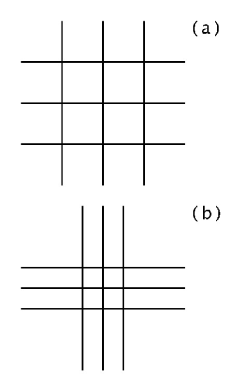
What is more, Minkowski Functionals are actually unsuited for What we are after here. Take the two very simple examples shown in Figure 1. Both cases contain six model filaments (that are much longer than wide), which form a simple network. They both yield the exact same Minkowski functionals, whereas they look different: In case a, each intersection is connected to four identical fragments, whereas in case b, each intersection is connected to either two short and two long or three short and one long or four short fragments. If we take Figure 1 as a very simplistic model case for the inter–cluster filaments studied in Colberg et al. (2005), it becomes obvious that Minkowski functionals lack predictive power to tell the difference between the two cases.
The aim of this work is to locate structure elements of LSS and to describe their properties. This is done by running a group finder on haloes from a very large and very detailed N–body simulation, and by then directly determine the actual geometrical structure of those objects. The algorithm consists of the application of well–known techniques such as a friends–of–friend group finder and a Minimal Spanning Tree (MST) plus a new way to categorize the MST and to extract its branches and their properties. We will then apply the algorithm to the simple test cases shown above and to the full set of haloes from the Millennium Run simulation (Springel et al. 2005).
This paper is organized as follows. In the following Section (2), we first briefly introduce the simulation data used in this work. In Section 3, we discuss the algorithm to find cosmic structures, which consists of using a group finder (Section 3.2), a Minimal Spanning Tree (Section 3.3), and a new algorithm to classify the elements of the latter (Section 3.4). In Section 4, we present results of the study, namely numbers of structural elements (Section 4.1), their shapes (Section 4.2), and their spatial extents (Section 4.3). Section 4.4 contains a study of the mass dependence, and in Section 4.5, we study the influence of sampling. Finally, in Section 5 we discuss the findings of the study.
2 The Simulation
2.1 Simulation Details
We make use of the halo catalogue obtained from the Millennium Run, a very large dark–matter–only N–body simulation of the concordance CDM cosmology with 21603 particles in a (periodic) box of size 500 Mpc in each dimension. The cosmological parameters are total matter density , dark energy/cosmological constant , Hubble constant , and the normalization of the power spectrum . With these parameters, each individual dark matter particle has a mass of M⊙. See Springel et al. (2005) for more details of the simulation.
2.2 Haloes and subhaloes
The simulation code was designed to produce friends–of–friends (FOF) group catalogues on the fly and to output these along with particle data at each output time. FOF groups are sets of particles in which any pair’s separation does not exceed some fraction of the mean inter–particle separation (Davis et al. 1985, but also see the earlier application in Turner & Gott 1976). With a choice of , the groups have mean overdensities of about 200, which roughly corresponds to that expected for a virialized group. There are FOF groups in the simulation volume, each with 20 particles or more.
Given the very high mass resolution of the Millennium Simulation, the haloes contain substructures, which, however, are not resolved with the FOF group finder. To find the substructures, an improved and extended version of SUBFIND (Springel et al. 2001) was applied. That way, a total sample of subhaloes was found. Here, a halo is counted as a single subhalo if it does not contain any identifiable substructure. The largest halo contains 2328 subhaloes. For more details on the group finding again see Springel et al. (2005).
3 Finding Large–Scale Structures
3.1 Overview: Locating Cosmological Superstructures
The procedure described in the following aims at locating structures in the Millennium Run simulation in such a way that the structure elements agree with those found by eye (for interesting discussions of this see Barrow & Bhavsar 1987 and Bhavsar & Ling 1988b). With such a seemingly vague ansatz there are no obvious physical criteria on how to proceed. It would be tempting to adopt simple toy models and to base the procedure on those. However, cosmological structures appear to be far more complicated than a simple mix of simplified cylinders (filaments) and sheets (walls); and we want to avoid biasing the study by relying on too simple models.
What the eye (or rather the brain) does is to take the massive clusters as nodes of the network, and it classifies the chains of haloes in between them into different categories, depending on where they lie and how close they are to their neighbours. Here, we will mimick this kind of classification as follows:
-
1.
Groups of haloes are found using a standard fof group finder for the full halo sample. Given the fact that the linking length is a free parameter, this procedure will be repeated with different choices for the linking length. We focus our attention to the parameter range where the vast majority of haloes ends up in one big group.
-
2.
The haloes in the largest group are assigned to a three–dimensional grid. The size of its cells are chosen on the basis of the smallest scales to be resolved. We here pick 2 Mpc in each dimension, since we are only interested in the large–scale distribution of matter. Note that this step reduces the computational complexity of the following steps by decreasing the number of the data points.
-
3.
We construct the Minimal Spanning Tree (MST) for those cells that contain at least one halo. The technical details of a MST will be discussed further below; briefly summarized a MST is a data structure that contains nodes (in our case grid cells containing haloes) and connections (so–called edges) between them, with the sum of the lengths of the edges being minimal.
-
4.
We classify the nodes of the MST according to their position inside the MST as major and minor nodes (again, details below). The former are nodes such as those formed by massive galaxy clusters. These lie at the intersections of filaments and sheets, where the latter can be found.
-
5.
Having classified the MST that way, we end up with a hierarchical data structure of branches and subbranches, from which we can determine the sizes and shapes of structure elements quite easily.
In the following Sections, we will discuss the individual steps in more detail.
3.2 Group Finding
The first step of the procedure to find LSS elements is to run a standard FOF group finder on the halo catalogue. For the linking length333Note that for large haloes we use their subhaloes for the group finding. Since the virial radii pf cluster–size haloes are larger than the linking length, using only haloes would exclude those haloes from the search. Using the subhaloes solves this problem., we adopt a variety of fractions of the mean interhalo separation Mpc, ranging from values between 0.5 and 0.6. Our choice of linking length is motivated by the following.
Between values of 0.5 and 0.6 times the mean inter–halo separation, we witness the onset of percolation: Initially, the largest object contains only a couple of percent of the total (halo) mass. The fraction of mass in the largest objects then grows very rapidly to finally reach 70% of the total mass (see Table 1). For point distributions, this process has not been studied in much detail since Dekel & West (1985) concluded that the strong dependence of the onset of percolation on the mean density of the sample ruled out its use as a tool to study LSS. For earlier applications of percolation to study cosmic structures see the seminal papers by Bhavsar & Barrow (1983), Einasto et al. (1983), and Shandarin (1983), also Klypin & Shandarin (1993).
For the present study, the exact choice of linking length does not matter as long as we stay in the regime where the largest object contains a significant amount of LSS. We will later study systematic effects such as different linking lengths or different halo sample sizes.
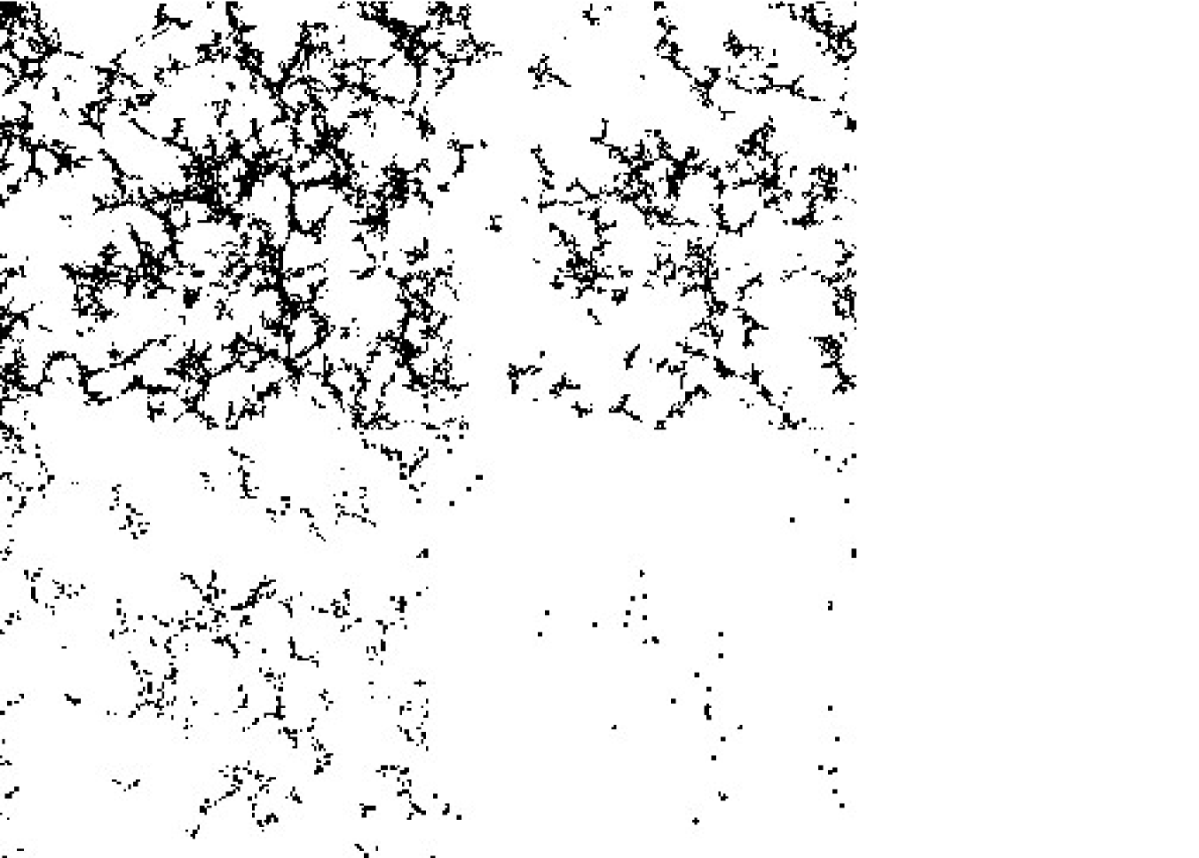
The upper–left panel of Figure 11 shows a slice of thickness 15 Mpc through the simulation volume, with the sizes of the symbols reflecting the halo masses. The symbols show haloes that are part of the largest object at 60% of the mean interhalo separation. Note that because this image shows a thin slice through the volume, the largest object appears to be broken up into separate pieces. With this choice of linking length, the largest object contains 69.4% of the total mass.
Since we are interested in the sizes and shapes of structures on large scales we bin the haloes of each group onto a three–dimensional grid with a cell size of (2.0 Mpc. We represent each grid cell that includes at least one halo by a single particle whose position corresponds to the center of the cell.
3.3 Minimal Spanning Trees
Twenty years ago, Barrow et al. (1985) introduced the Minimal Spanning Tree (MST) into the astronomical context. Initially thought to be an interesting tool, MSTs have not been used much over the course of the past ten years (see, for example, Bhavsar & Splinter 1996, Krzewina & Saslaw 1996, Doroshkevich et al. 2001, Demianski & Doroshkevich 2004), probably because of appeal of Minkowski Functionals and derived quantities. Bhavsar & Ling (1988) used MSTs to identify filaments in the CfA catalog, providing the first statistical evidence for the existence of filaments.
A Minimal Spanning Tree is a technique from graph theory (for the following brief review also see Barrow et al. 1985 and references therein). A graph is a collection of nodes (in astronomical cases typically galaxies), edges (straight connections between nodes), and edge lengths. A path is a sequence of edges that join nodes. A closed path is called a circuit; and a graph is called connected if all points are included in a path. A connected graph without any circuits is called a tree. If the tree of a connected graph contains all nodes, the tree is called a spanning tree. A tree’s length is defined as the sum of the edge lengths. The minimal spanning tree then is the spanning tree whose length is smallest. If no two edge lengths are equal the MST will be unique444Given that we are working with grid–based data, the MST in this work is not unique. We ran some tests with different MST’s that all represented the same data to find no differences in the properties of the structure elements constructued by our algorithm.. For more details on MSTs please c.f. Barrow et al. 1985 and references therein.
There are a few reasons why we are using the MST of the groups of haloes. Most importantly, by construction a MST does not contain any loops. This property is of crucial importance for the algorithm to locate branches of the tree, as will become clear in the following.
3.4 Locating Tree Elements
Once we have computed the MST we can apply our algorithm to find the branches. In the past (see, for example, Barrow et al. 1985), MSTs were typically pruned and broken apart. Smaller branches were cut off, and the MST was broken into pieces by removing the links between nodes that are connected by an edge of some given length. We will refrain from doing this here.
The idea behind the algorithm is very simple: The algorithm is designed to locate branches in such a way that smaller branches are part of larger ones and the whole tree is divided into branches naturally.
A detailed discussion of how the classification algorithm works can be found in the Appendix. Briefly summarized, the algorithm visits each node in the MST, and it determines the relation of the node to its neighbouring nodes. Depending on their numbers of neighbours, nodes are grouped into branches, with smaller branches becoming members of larger ones.
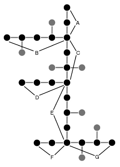
After the classification of nodes and the creation of hierarchical sets of branches, the code categorizes the structure by dividing it into major and minor branches. Major branches are those that are longer than a given (arbitrary) length . This procedure is the equivalent of pruning an MST. Figure 2 shows a very simple example.
For the analysis of the halo groups, we choose Mpc or five mesh cells. But note that with this procedure major branches can be shorter than Mpc. This will be the case for those branches that lie inside the structure and have no loose end.
3.5 Simple Test Cases

As a proof of concept, we first apply the structure–finding algorithm to the two cases shown in Figure 1. Case and consist of six long intersecting lines each, with nine vertices. These intersections divide the lines into segments, and it is these segments that the algorithm finds.
For both cases, we created a set of 120,000 model particles, which we distribute randomly, following the spatial patterns shown in Figure 1. For case , the spacings of the model filaments were chosen to be 100 Mpc. For case , the filaments were spaced 50 Mpc apart. Thus, in case , the segments all have the same length (100 Mpc), whereas in case , half the segments have a length of 50 Mpc and half are 150 Mpc long.
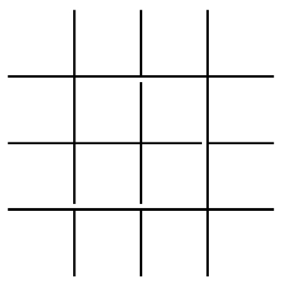
Figure 3 plots the size distributions of the major branches measured for the model particle distributions for case (solid histogram) and (dashed histogram). As can be seen from the Figure, our algorithm identifies the different segments as major branches and exactly reproduces their size distributions. It needs to be stressed that the two cases as shown in Figure 1 are not MST’s555Remember that an MST does not contain any closed loops!. As an example, Figure 4 shows the MST constructed by our code for case (a). The code placed the small gaps needed to convert the graphs from Figure 1 into MST always right next to the vertices, which led to the exact reproduction of the size distributions. In principle, it is possible that the code will break a connection between vertices somewhere in the middle, thus breaking a structure element into two pieces. It is impossible for us to exactly quantify to what extent this is actually happening in the vastly more complex cases from the simulation discussed below. However, it is not likely that the misidentification of structure elements as broken pieces will lead to a significant distortion of our results, since the structure of the graphs used as simple test cases from Figure 1 is much simpler than those of actual simulation data. There, unlike in the toy models, loop–like structures formed by haloes tend to contain a very large number of individual structure elements. Breaking some of them into two pieces will thus introduce only a very small error.
In addition to the two simple cases shown in Figure 1, we tested the algorithm on a number of more complex, fully three–dimensional geometric configurations of model particles. In each of those cases, the algorithm was able to determine the correct numbers, shapes, and sizes of the individual structure elements.
We now apply the structure finding algorithm to the Millennium Run halo sample and study the results.
| 0.50 | 2.1% | 1191 |
| 0.51 | 6.9% | 4175 |
| 0.52 | 14.2% | 9543 |
| 0.53 | 29.9% | 21288 |
| 0.54 | 38.5% | 29485 |
| 0.55 | 47.4% | 38591 |
| 0.56 | 53.5% | 46059 |
| 0.57 | 58.2% | 53422 |
| 0.58 | 62.5% | 60584 |
| 0.59 | 65.9% | 67282 |
| 0.60 | 69.4% | 74086 |


4 Results obtained for Millennium Run halo samples
Table 1 summarizes the fraction of the total halo mass contained in the largest object and the number of major branches as a function of the linking parameter . The effect of percolation is shown in Figure 5 (c.f. Section 3.2). rises from just a couple of percents at to almost 70% at . We also find that at any the largest object always is much larger than the second largest or any other object in the volume.
4.1 Numbers of structure elements
As we increase , so does the number of haloes in the largest object. Figure 6 shows how this increase in size translates into the number of major branches. At the largest , there are more than 74,000 major structure elements present. This finding impressively confirms the immense complexity of LSS.
At and above the relation between and is almost linear. The growth of the largest object around the percolation threshold can be understood as follows. As as the linking length increases, a larger and larger number of formerly disjoint objects that gets interconnected. The linear relationship between and in Figure 6 clearly reflects this process. We will study next whether the properties of these major branches change with .
4.2 Shapes of major branches
To study the shapes of the branches666In the following, branches will stand for major branches. for we compute the quantity
| (1) |
for the centers of their cells, where the sum is over all cell centers. The normalized eigenvectors of correspond to the unit vectors of the best–fit ellipse of the branch, and there are three eigenvalues, sorted such that . This procedure is commonly used for the shapes of haloes (see, for example, Hopkins et al. 2005 and references therein). Note that because of the relatively small number of cells per node777For example, for the sample, the largest major branch contains only 162 cells. Typically, is computed for haloes, which – depending on the simulation details – contain many thousands of particles. provides only a fairly crude measure of the shapes of those branches. We will not be able to determine more than whether branches are roughly filamentary, sheet–like, or elliptical.
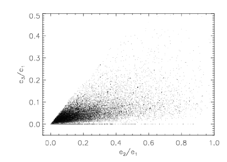
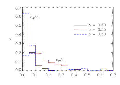
Figure 7 shows versus for the largest sample (). Because the area with is empty. Note the different scales of the and –axis. The vast majority of major branches has , which means that they are planar or close to planar. Because of the nature of the branches some are even completely straight.
In Figure 8, we plot the fractional distributions of and for the three different halo groups (solid line), (dotted line), and (dashed line). As already seen in Figure 7, just a few percent of branches have . The distribution of is broader. However, only a few percent of the branches have . and corresponds to straight or slightly curved filaments.
In addition to comparing the fractional distributions of and , Figure 8 also compares halo groups for different linking lengths . There are no discernable differences between the samples. The mean values of these quantities for the different samples , 0.1734, and 0.1736 and , 0.0437, and 0.0428 for , 0.55, and 0.50, respectively.
In a sense, the results obtained for the shapes of branches are not very surprising. Haloes that comprise the largest object at are also contained in the largest object at larger . This statement is not trivial, though. It is possible to have a distribution where the haloes in the largest object at , say, are not contained in the one at . 888This could happen if at a group of smaller objects from connect to form the largest object. However, this is not the case for our sample..
Given the results so far, LSS thus can be understood as being composed of a fixed set of building blocks, with different sizes and shapes, very much like a set of cosmic Lego bricks. Depending on how one chooses the linking length, the largest object is constructed by picking the same pieces, albeit in different numbers.
| sample | Mpc] | |
|---|---|---|
| full sample | 71,064 | 9.1 |
| 15730 | 12.6 | |
| 2431 | 25.7 | |
| 193 | 64.4 |
4.3 Spatial extents of major branches
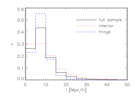
Figure 9 shows the distributions of spatial extents of major branches. By spatial extent we here mean
| (2) |
for each major branch, where (, , ) and (, , ) are the minimum and maximum coordinates of the major branch, respectively. For perfectly straight branches is the actual length of the branch, for a branch that forms two sides of a rectangle, is the length of the diagonal, etc.
We also divided the major branches into two categories. The first category (interior) contains those branches that connect to two (or more) major branches at each end. The second category (fringe) encompasses those that connect to two (or more) major branches only at one end. In other words, the latter branches have a loose end. For example, in Figure 2, branches A, B, D, F, and G belong to the second category, whereas only branches C and E are category one branches.
For the Millennium Run haloes, the numbers of branches in the two categories are roughly equal. Figure 9 shows the distributions of for all (solid line), interior (dotted line), and fringe (dashed line) branches (). Fringe branches appear to be shorter than interior ones.
About two thirds of the major branches have extents of up to Mpc. The other third extends to larger scales, with a very small number going beyond Mpc.
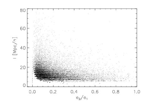
In Figure 10 we plot versus for the sample. Below Mpc the effect of the grid is clearly visible as horizontal stripes. There appears to be a tendency for shorter branches to have a broader distribution in . This trend is almost entirely caused by how the ’s are computed. The shortest branches consist of only a few cells, and thus their shapes have to be taken with a grain of salt. However, there is a general trend for more extended branches to be more filamentary999Remember that tends to be much smaller than – see Figure 8..
4.4 Halo Mass Dependence
Having examined the properties of LSS formed by the full set of haloes, we now turn our attention to subsamples. From the original halo set we construct three subsamples by requiring minimum masses of , , and . Very crudely, these masses correspond to those of late–type galaxies, groups of galaxies, and massive galaxy clusters, respectively. In the following, we will refer to these samples as m12, m13, and m14.
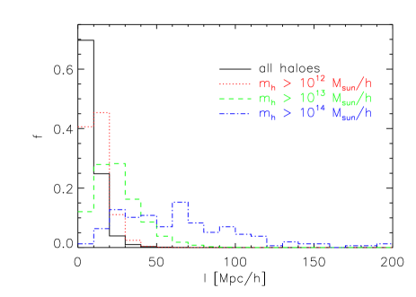
In Figure 11, we show a slice through the simulation volume, displaying only haloes that are part of the largest object. The upper left, upper right, lower left and lower right panel correspond to the full halo sample, and samples m12, m13, and m14, respectively. In order to build the largest object we chose the individual linking lengths for the group finding in such a way that for each sample, the largest object contains about 65% of the total mass in the halo sample. Table 2 summarizes the four samples; in the second column, the total number of haloes is quoted.
For each sample, we run the structure finder on the largest group and compute properties of the major branches. Columns three and four of Table 2 give the total number of major branches and their mean extent, respectively. As could be expected, the larger the minimum mass of the halo sample, the larger the mean extent of major branches.
This effect is also visible in Figure 11. More massive haloes (sample m14) can be predominantly found in overdense regions, and the bridges between them – formed by less massive haloes – are replaced with simple connections. In other words, many of the nodes visible in the upper panel of Figure 11 disappear as the mass threshold is increased, and for sample m14 only the most massive nodes are left.
Figure 12 provides a more detailed view of the extents of major branches. It shows histograms for the four samples. The extent of major branches in sample m14 extends all the way up to a maximum value of 191.5 Mpc. Very long, connected chains of massive haloes are thus a feature of simulations of cosmic structure formation. This fact is particularly reassuring in the light of observations of very extended chains of galaxies and of cosmic superclusters and superstructures (see, for example, Bharadwaj et al. 2004 or Gott et al. 2005). Images of the LSS in the simulation (Figure 11) clearly support the finding that there are coherent structures of this size. It is thus highly unlikely that the sizes of the structure elements in the m14 sample are due to sparse sampling.
| sample size | ||
|---|---|---|
| full sample | 0.649 | 0.600 |
| 50% | 0.651 | 0.654 |
| 25% | 0.650 | 0.699 |
| 10% | 0.652 | 0.753 |
4.5 Sampling Issues
Having computed the extents of major branches both for the full halo sample and for subsamples chosen by mass, it is important to test how sample completeness affects the results. Before doing this we need to address an important issues which might be raised as an objection to the methods presented here.
Examining randomly selected subsamples of the haloes provides a test of the structure finding algorithm only if we make sure that similar objects are being compared. In the following, we will investigate objects that contain 65% of the mass of each sample. As noted above, if the percolation of a set of points is studied, there is a dependence of the percolation threshold on the density of the point sample. What this means in a cosmological context is that if there are two samples of points with the same two–point correlation function but different densities, then the percolation threshold for the samples will be different. The sample with the lower density will have a higher percolation threshold. One can show that for very sparse samples, the percolation behaviour is that of a Poisson distribution (see Dekel & West 1985).
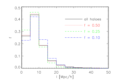
Table 3 summarizes the properties of the different halo samples used for this test. As can be seen from the first and last column, as the number density of the halo sample decreases, the factor needed to scale the mean inter–halo separation for the group finding increases.
In Figure 13, we plot the extent distributions of the major branches in the samples from Table 3. There is almost no difference between the full sample and the one containing only half the haloes. For even smaller subsamples, the differences in the distributions are small, with no apparent systematic trend. Whereas the 25% subsample appears to favour slightly smaller major branches, the 10% subsample follows the opposite trend, with both deviating from the full sample distribution by small factors only.
We thus conclude that while the downsampling affects the percolation behaviour of the resulting halo samples, it does not change the basic properties of LSS as measured by our structure–finding algorithm – provided the comparison is done in such a way that the largest object contains the same mass fraction in the different samples. This conclusion is supported by the earlier results obtained by Bhavsar & Splinter (1996).
5 Summary and Discussion
We introduced a new algorithm to classify cosmic structures. This algorithm is based on a Minimum Spanning Tree representation of groups of haloes that are found with a standard FOF group finder. The new algorithm exactly reproduces the length distributions of filaments in a set of simple test cases.
Structures like the one shown in Figure 11 contain many thousands of structural elements, which in the context of this work were called major branches. We investigated the numbers and properties of these objects using haloes from the Millennium Run simulation (Springel et al. 2005). For the group finding linking lengths between and 0.6 were employed, around the percolation threshold. For each linking length, we concentrate on the largest object. We find that while the fraction of mass in the largest object and the actual number of its major branches are a function of , the properties of those branches do not change101010Note that the linking length, in physical units, in this range changes from 1.005 Mpc to 1.206 Mpc or 2.01% to 2.41% of the size of the simulation volume in one dimension, while the fraction of halo mass in the largest object jumps from 2.1% to 69.4% – the tell–tale sign of percolation..
We then computed quantities for the major branches that correspond to shapes and extents. Branches are predominantly planar, with straight or curved filamentary configurations preferred. A small number of branches appears to have significant extents in two dimensions. The shapes of the major branches are independent of the choice of . This means that cosmological percolation, while leading to a vast increase in the size of the object, does not alter its structural properties. Instead, as increases, more and more pieces of the same kind are being added to the largest object.
Large Scale Structure thus appears to be modular, with a fixed set of pieces – with different sizes and shapes. This finding adds considerable information to the earlier study by Colberg et al. (2005), who investigated inter–cluster filaments. Note that here, we have not made any assumptions on where to look for filaments (or sheets). Given the difference in method, the general agreement between size distributions found here and in Colberg et al. (2005) is quite interesting. There, it was found that clusters with separations of up to 15 Mpc almost always have a filament between them. Here, we find that the vast majority of branches have extents of up to 15 Mpc.
It is reassuring that the results of this study support the visual impression from images like the one shown in Figure 11: LSS in N–body simulations consists predominantly of a complex network of filamentary structures. This work represents the first systematic attempt to determine numbers, sizes and shape distributions of structure elements.
Different halo samples, chosen by mass, exhibit a correlation between the minimum mass of the sample and the mean extent of the resulting major branches. The larger the threshold mass, the longer the major branches. Massive galaxy clusters form the backbone of LSS. It is reassuring to see that despite the differences between the methods employed here and in Bharadwaj et al. (2004), the largest structure elements extend over many dozens of Megaparsecs. With the longest single coherent structure element in the sample being almost 200 Mpc in length, the simulation appears to be in good shape to account for very large features of LSS such as, for example, the SDSS Great Wall (Vogeley et al. 2004).
The properties of major branches in LSS appear to be quite unfazed by a downsampling of the halo sample to as little as 10% of the original size. For this test, for each halo we picked a linking length which led to the largest object containing about 65% of the total sample mass.
It is tempting to argue that the predominance of filaments and the small number of sheets/walls is caused by how we investigate structures. After all, it is possible that there are sheets in the simulation volume that the the algorithm breaks up into many straight and warped filaments. In principle, it is hard to see what is wrong with this argument. However, when we visually inspected the distribution of haloes and the largest object we were unable to find prominent sheets. However, it appeared that most structures that we would classify as sheets appeared to consist of a set of connected filaments with gaps in between them. What this means is that while there are regions of space that do contain large mass concentrations in a planar configuration, inside that plane the matter has already collapsed into individual filaments. This not only supports the results obtained here, but it also explains why studies using Minkowski Functionals and Shapefinders (see Sheth & Sahni 2005 and references therein) have not been able to find strong signals from sheets.
Finding an algorithm to classify LSS would be a mostly academic exercise if it was only applied to real–space haloes from Dark–Matter only simulations. This current work merely introduces the algorithm, along with some systematic tests. In a future study, we plan to apply the methods outlined here redshift–space data from mock galaxy catalogues and actual observed galaxy surveys.
Acknowledgments
The Millennium Run simulation used in this paper was carried out by the Virgo Consortium (http://www.virgo.dur.ac.uk) at the Computing Center of the Max–Planck–Gesellschaft in Garching, Germany. We thank Rupert Croft, Carlos Frenk, Tiziana di Matteo, Cameron McBride, Volker Springel, and Naoki Yoshida for helpful discussions and comments on earlier drafts of this work, and the anonymous referee for very helpful suggestions for improvements. Thanks are also due to Esther Jesurum for advice concerning advanced C++ techniques and to Rien van de Weygaert for providing his code used in to prepare an earlier version of the structure–finding code.
References
- [1] Babul A., Starkman G.D., 1992, ApJ, 401, 28
- [2] Barrow J.D., Bhavsar S.P., Sonoda D.H., 1985, MNRAS, 216, 17
- [3] Barrow J.D., Bhavsar S.P., 1987, QRAS, 28, 109
- [4] Bharadwaj S., Bhavsar S.P., Sheth J.V., 2004, ApJ, 606, 25
- [5] Bhavsar S.P., Barrow J.D., 1983, MNRAS, 205, 61
- [6] Bhavsar S.P., Ling E.N., 1988a, ApJ, 331, 63
- [7] Bhavsar S.P., Ling E.N., 1988b, PASP, 100, 1314
- [8] Bhavsar S.P., Splinter R.J., 1996, MNRAS, 282, 1461
- [9] Colberg J.M., Krughoff K.S., Connolly A.J., 2005, MNRAS, 359, 272
- [10] Colless M. et al., 2001, MNRAS, 328, 1039
- [11] Croton D.J. et al., 2005, astro–ph/0508046
- [12] Davis M., Efstathiou G., Frenk C.S., White S.D.M., 1985, ApJ, 292, 371D
- [13] Dekel A., West M.J., 1985, ApJ, 288, 411
- [14] Demianski M., Doroshkevich A.G., 2004, A&A, 422, 423
- [15] Doroshkevich A.G., Tucker D.L., Fong R., Turchaninov V., Lin H., 2001, MNRAS, 322, 369
- [16] Einasto J., Klypin A., Shandarin S., 1983, IAUS, 104, 265
- [17] Gott J.R., Dickinson M., Melott A.L., 1986, ApJ, 306, 341
- [18] Gott J.R., Juri M. Schlegel D., Hoyle F., Vogeley M., Tegmark M., Bahcall N., Brinkmann J., 2005, ApJ, 624, 463
- [19] Hopkins P.F., Bahcall N.A., Bode P., 2005, ApJ, 618, 1
- [20] Klypin A., Shandarin S.F., 1993, ApJ, 413, 48
- [21] Krzewina L.G., Saslaw W.C., 1996, MNRAS, 278, 869
- [22] Luo S., Vishniac E., 1995, ApJ, 96, 429
- [23] Luo S., Vishniac E., Martel H., 1996, ApJ, 468, 62
- [24] Mecke K.R., Buchert T., Wagner H., 1994, A&A, 288, 697
- [25] Peacock J.A., 1999, “Cosmological Physics”, Cambridge University Press, Cambridge, UK, ISBN 0–521–42270–1
- [26] Peebles P.J.E., Groth E.J., 1975, ApJ, 196, 1
- [27] Peebles P.J.E., “The Large–Scale Structure of the Universe”, Princeton University Press, Princeton, NJ
- [28] Sahni V., Sathyaprakash B.S., Shandarin S.F., 1998, ApJL, 495, 5
- [29] Shandarin S.F., 1983, PAZh, 9, 195
- [30] Shen J., Abel T., Mo H., Sheth R.K., astro–ph/0511365
- [31] Sheth J.V., Sahni V., 2005, “Exploring the Geometry, Topology and Morphology of Large Scale Structure using Minkowski Functionals”, to appear in Current Science, also astro-ph/0502105
- [32] Springel V., et al. (Virgo Consortium), 2005, Nature, 435, 629
- [33] Springel V., White S.D.M., Tormen G., Kauffmann G., 2001, MNRAS, 328, 726
- [34] Springel V. et al., 1998, MNRAS, 298, 1169
- [35] Tago E., Einasto J., Einasto M., Saar E., 2005, astro–ph/0501099
- [36] Turner E.L., Gott J.R., 1976, ApJS, 32, 409
- [37] Vogeley M.S., Hoyle F., Rojas R.R., Goldberg D.M., “Mapping the cosmic web with the Sloan Digital Sky Survey”, in: “Outskirts of Galaxy Clusters: Intense Life in the Suburbs”, proceedings of the IAU Colloquium 195, ed. Diaferio A., Cambridge University Press, Cambridge, UK, ISBN 0–521–84908–X
- [38] York D.G. et al., 2000, AJ, 120, 1579
Appendix A Locating Tree Elements
In a nutshell, structure elements of the MST are found by grouping its individual elements into larger units. These larger units are constructed on the basis of how the elements of the MST are interconnected. Before discussing the algorithm in detail, it is important that the notation used in the folowing is clear. Our starting configuration is a MST, constructed from cells on a grid. A node is simply such a cell, that is an individual member of the MST. An edge is a connection between two nodes. Each node is connected to at least one other node, and we will call the set of nodes that any given node is connected to its neighbouring node(s). As already mentioned, the algorithm groups nodes into larger units. Any such unit we will call a branch, and it might contain a collection of connected nodes and other branches. Each branch has to contain at least one node. If a branch contains other branches then the longest of those branches will be called the main branch, with the remaining one(s) being subbranches. A branch is represented by the last node added to it.
It is probably easiest to understant the classification algorithm by referring to Figure 14, which schematically depicts the application of the algorithm to a very simple case. Figure 14 shows the same MST at six different steps of the algorithm. As the individual nodes are being grouped into units, the different branches are shown as grey boxes around the nodes and edges they consist of.
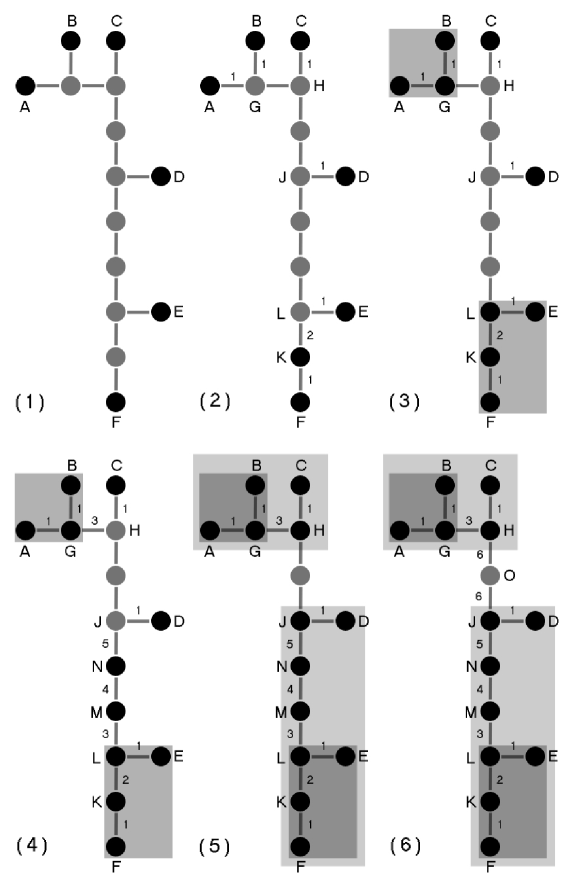
The algorithm constructs branches from the MST’s nodes and edges using a simple set of rules. The rules are applied sequentially until each node is contained in at least one branch.
The initial set of branches is constructed from all nodes that are connected to only one other node – the loose ends of the structure. In Figure 14, these are nodes A to F. In order not to make Figure 14 too cluttered, there are no grey boxes drawn around these initial branches.
Using the set of initial branches, the full classification of the MST is done by applying the following rules:
-
1.
As mentioned before, a branch is represented by the node that was added last. Take all branches that are not contained inside another branch and take their representing nodes. For those nodes, find their neighbouring nodes. If a neighbouring node can only be added to one node’s branch (and to no other branch) add it to that branch, and make it the new representing node of the branch. Increase the length of the branch accordingly.
-
2.
If a neighbouring node can be added to more than one branch, set the node and the branch aside in a queue, and ignore this branch for the time being.
-
3.
For each branch, add only one neighbouring node at a time.
-
4.
Go back to the first step if (and only if) there are other nodes that can stil be added to a branch.
-
5.
If no node can be added to any branch, process the branches and nodes in the queue. At this stage it is important to realize that each node that does not sit at the edge of the MST can be connected to a number of other nodes, and by construction of the algorithm, . What this means is that a node can potentially reside at the intersection of branches. In this step, the goal is to process all nodes for which there are either or neighbouring branches contained in the queue, with the latter case only possible at the very end of the algorithm. Nodes for which less than neighbouring branches are in the queue are ignored.
In the case where there are branches in the queue for a node consolidate these branches and the node as follows. Create a new branch, represented by the node, and add the branches as subbranches to the new branch. Find the longest subbranch from those and label it as the main subbranch. The length of the new branch is taken as the length of the main subbranch.
As already indicated, the case will only be met once, at the very end of the algorithm (if this point is not clear, it will become clear below, where we will discuss the simple example from Figure 14). The node and the branches in the queue are processed just like in the , with the only differences being that a) the length of the final branch is taken as the sum of the two longest subbranches (there are at least two subbranches), and b) there is no more work left to do, so the algorithm is finished.
-
6.
After the queue has been cleaned up as far as possible continue adding the remaining nodes (if there are any left) by going back to the first step.
It is probably worth discussing how the algorithm is applied in the case of the simple MST depicted in Figure 14. Please keep in mind, though, that real cases will be threedimensional, and edges will not all have the same length.
As already mentioned, step (1) in Figure 14 shows the identification of the initial set of branches by locating the loose ends of the structures. These are the nodes labeled A to F.
Step (2) shows the application of rules (i) to (iv). For example, node F is connected to node K, which at this stage can only be added to F and to no other node. K is thus added to the branch and made the new representing node. At nodes G, H, J, and L, rule (ii) applies. After the first iteration, there is only one free node left to process, node K. Its neighbour, L, sits at an intersection, so rule (ii) applies. After this step, all nodes that have not been added to a branch (G, H, J, and L) are inside the queue, and no free branch can be added anywhere.
Step (3) shows the application of rule (v). Figure 14 shows that rule (v) describes how to deal with intersections, where several branches meet at a node. In step (3), shaded boxes indicate which parts of the queue can be processed. The case of node J is quite obvious. Node H cannot be processed, yet, since node G itself is inside the queue. Nodes G and L can be processed. At node G, two branches of the same size meet, and one of them is picked as the main subbranch randomly. The new branch contains the nodes A, B, and G, and two subbranches, namely A–G and B–G. It is represented by node G. At node L, two branches with different sizes meet, with F–K–L being longer than E–L. The new branch also has two subbbranches, with the main subbranch given by F–K–L, and the new branch is represented by node L.
At step (4), we are back at applying rules (i) to (iv). At H, rule (ii) applies immediately. From node L onwards, we can make our way towards node J (rules (i), (iii), and (iV)), at which point rule (ii) applies.
The remaining steps contain only one slightly difference, namely at step (6), when processing the queue at node O, we are done. The final branch contains all nodes and the subbranches constructed earlier, and the length of the final branch is given by the length of the chain of nodes starting at A, going to H and then down to F. We will refer to node O as the base node.
As Figure 14 shows, the classification of the MST is done outside–in, that is the classification of the nodes into branches is done such that larger branches are built from smaller ones.
Once the MST has been categorized into sets of branches and subbranches, we construct another, somewhat simpler data structure from it. Starting at the base node major branches of the structure as follows: We build a new set of branches by now moving away from the base node and by adding nodes to these branches. Whenever we run into a node where the tree bifurcates, we ignore those subbranches that are shorter than some length scale . The value of is an arbitrary pruning parameter (in the fashion of the pruning parameter used for MSTs discussed in Barrow et al. 1985). If there are two (or more) subbranches at some node which are longer than , we create two new branches, add those to the current branch, and then we walk down those two (or more) branches. It needs to be said that this step really is just amounts to a rearrangement and slight pruning of the first classification.
Figure 2 shows an example of a simple tree, with its major branches marked (nodes that belong to a major branch are shown in black) and labeled (A to G). In this example, a subbranch is required to have length 2. Otherwise, its nodes will not be contained in any of the major branches. Note that the major branches, unlike the branches in the original tree constructed from the MST, only contain nodes/edges. The major branches are designed to represent the major structural elements in the tree.