Non-axisymmetric instability and fragmentation of general relativistic quasi-toroidal stars

Abstract

In a recent publication, we have demonstrated that differentially rotating stars admit new channels of black hole formation via fragmentation instabilities. Since a higher order instability of this kind could potentially transform a differentially rotating supermassive star into a multiple black hole system embedded in a massive accretion disk, we investigate the dependence of the instability on parameters of the equilibrium model. We find that many of the models constructed exhibit non-axisymmetric instabilities with corotation points, even for low values of $T/|W|$, which lead to a fission of the stars into one, two or three fragments, depending on the initial perturbation.

At least in the models selected here, an $m=1$ mode becomes unstable at lower values of $T/|W|$, which would seem to favor a scenario where one black hole with a massive accretion disk forms. In this case, we have gained evidence that low values of compactness of the initial model can lead to a stabilization of the resulting fragment, thus preventing black hole formation in this scenario.

I Introduction

The study of oscillations and stability of stars has a long history (see e.g. Tassoul (1978)). While its classical results tried to address the limits of possible models for main-sequence stars, and the question of binary star formation from protostellar clouds, it has been extended in the last century to examine the properties of relativistic fluid equilibria, and their connection to the formation of black holes by axisymmetric instabilities.

This work is an extension of our publication Zink et al. (2006a), where we have studied the formation of black holes from fragmentation in $N=3$ polytropes, which was induced by the growth of a non-axisymmetric instability in a strongly differentially rotating star. We would like to focus attention here on the question of whether the instability we have observed is generic for strongly differentially rotating polytropes, and how changes in parameters of the initial model affect its development. In addition, we will present some tentative results related to arguments previously presented by Watts et al. Watts et al. (2005) on a possible connection between low-$T/|W|$ and spiral-arm instabilities and the location of the corotation band in a sequence of increasing rotational energy.

Due to the recent prospect of detecting gravitational radiation directly, the connection between the local dynamics of collapse and gravitational wave emission is currently receiving increased attention (e.g. Thorne (1997); Baiotti et al. (2005a)). In this context, a non-axisymmetric instability in a star is expected to change the nature of the signal, and to enhance the chances of detecting it Houser et al. (1994). We shall discuss a number of scenarios for gravitational collapse and black hole formation to illustrate this point.

1. Stars retaining spherical symmetry: If the initial matter distribution has spherical symmetry, no gravitational waves are emitted as a consequence of Birkhoff’s theorem. The exact solution by Oppenheimer and Snyder Oppenheimer and Snyder (1939) already exhibits many features of the local dynamics, while the connection to dynamical stability in general relativity has been made explicit by Chandrasekhar Chandrasekhar (1964). The assumption of spherical symmetry, whilst restrictive, already admits simple models of phenomena like mass limits for compact stars, some generic properties of black hole formation from supermassive stars and neutron stars (e.g. May and White (1966); Shapiro and Teukolsky (1979, 1980)), and the dynamics of apparent and event horizons (ibido).

2. Stars retaining (approximate) axisymmetry: If the symmetry assumption is relaxed to axisymmetry, models of gravitational collapse admit a number of additional features, the most important in this context being the emission of gravitational radiation. Stars in axisymmetry can be rotating, which changes the radial modes of the non-rotating member of a sequence into a quasi-radial mode. If that is unstable, the star may collapse to a black hole in a manner which is similar to the spherically symmetric case in its bulk properties, and it proceeds by (i) contraction due to a quasi-radial instability, (ii) formation of an event horizon centered on the axis, and (iii) ring-down to a Kerr black hole with a disk. We will call this process the canonical scenario to represent that it provides the expected properties of the collapse of slowly rotating stars. It has been studied extensively in numerical investigations Nakamura et al. (1980); Nakamura (1981a, b, 1983); Stark and Piran (1985); Shibata (2000); Shibata et al. (2000a); Saijo et al. (2002); Shibata and Shapiro (2002); Font et al. (2002); Shibata (2003); Duez et al. (2003, 2004); Baiotti et al. (2005a); Saijo (2004); Baiotti et al. (2005b), and seems even appropriate to describe the quality of collapse of most rapidly and differentially rotating neutron stars Duez et al. (2004). It should not be considered implicit here that the canonical scenario is generic for axisymmetric collapse: see e.g. Hughes et al. (1994); Abrahams et al. (1994) for systems involving toroidal black holes.

3. Stars not retaining (approximate) axisymmetry: As already mentioned, even in many numerical models with three spatial dimensions, the collapse to a black hole proceeds in an almost axisymmetric manner, although the initial data is represented on discrete Cartesian grids. It has been found that even when non-axisymmetric perturbations are applied to the collapsing material, no large deviations from axisymmetry are seen during the collapse Saijo (2004). Judging from the perturbative theory of Newtonian polytropes Tassoul (1978), this indicates that either the amount of rotational over gravitational binding energy $T/|W|$ is insufficient, or that the collapse time is too short to admit growth of initial deviations from the symmetric state to significant levels.

   The situation can be quite different when the system is not unstable to axisymmetric perturbations, or if the collapse stabilizes around a new equilibrium with higher $T/|W|$. The classical limit of $T/|W|\approx 0.27$ for Maclaurin spheroids Chandrasekhar (1969) indicates the onset of a dynamical instability to transition to the $x=+1$ Riemann S-type sequence Chandrasekhar (1969); Christodoulou et al. (1995). To which extent this idealized behaviour is also realized in general relativistic compressible polytropes, and, more specifically, how it is connected to the formation of black holes, is the issue we would like to address in part here.

If a general relativistic star encounters a non-axisymmetric instability, the nature of its subsequent evolution may be characterizable by certain properties of the equilibrium model, like the rotation law, $T/|W|$, compactness, and equation of state. For the limit of uniformly rotating, almost homogeneous models of low compactness, we expect, for $T/|W|>0.27$, a dynamical transition to an ellipsoid by a principle of correspondence with Newtonian gravity.

By relaxing all but the assumption of low compactness, we can make use of the rich body of knowledge about the stability and evolution of stars in Newtonian gravity. Two classical applications of stability theory are the oscillations of disks and the fission problem Tassoul (1978). These matters have been investigated extensively over the last decades Tohline et al. (1985); Durisen et al. (1986); Tohline and Hachisu (1990); Bonnell and Bate (1994); Loeb and Rasio (1994); Bonnell and Pringle (1995); Pickett et al. (1996); Houser and Centrella (1996); Rampp et al. (1998); Brown (2000); Imamura and Durisen (2001); Centrella et al. (2001); Colpi and Wasserman (2002); Davies et al. (2002); Imamura et al. (2003); Banerjee et al. (2004), and a number of possible scenarios have emerged for the non-linear evolution of non-axisymmetric dynamical instabilities in rotating polytropes:

1. The polytrope develops a bar-mode instability similar to the Maclaurin case, and possibly retains this shape over many rotational periods (e.g. Brown (2000)).

2. Two spiral arms and an ellipsoidal core region develop, where the latter transports angular momentum to the spiral arms by gravitational torques, is spun down, and collapses (e.g. Durisen et al. (1986)). This scenario is interesting for black hole formation, since the rotational support of the initial model can be partially removed by such a mechanism. If this transport is efficient enough, the core ellipsoid might collapse, resulting in a Kerr black hole with a disk of material around it. One might conjecture that, if the equation of state is soft enough, the disk itself may be subject to fragmentation, and form several smaller black holes which are subsequently accreted.

3. One spiral arm develops, and the mode saturates at some amplitude Pickett et al. (1996); Ott et al. (2005), leaving a central condensation. This might also lead to central black hole formation. Note that the onset for this dynamical instability in terms of $T/|W|$ can be significantly lower than the Maclaurin limit.

4. For polytropes with strong differential rotation, the initial model may be quasi-toroidal, i.e. it has at least one isodensity surface which is homeomorphic to a torus. If models of this kind, or purely toroidal ones, are subject to the development of a non-axisymmetric instability, they may exhibit fragmentation Rampp et al. (1998); Centrella et al. (2001). This is clearly the most interesting setting for the fission problem, but has been discussed also in the context of core collapse (“collapse, pursuit and plunge” scenario, Fig. 24.3 in Misner et al. (1973), also Bonnell and Pringle (1995); Davies et al. (2002)).

It is this last kind of instability we will investigate here in the context of general relativity, and its relation to the formation of black holes.

Concerning the nature of the spiral-arm and low-$T/|W|$ instabilities, Watts et al. (Watts et al. (2005), see also Watts et al. (2003, 2004)) have suggested a possible relation of these instabilities to their location with respect to the corotation band. That corotation has a bearing on instabilities in differentially rotating disks has been suggested for some time; the perturbation operator is singular at corotation points, which gives rise to a continuous spectrum of “modes.” While the initial-value problem of perturbations associated with the continuous spectrum of stars is not well understood even in Newtonian gravity, there is evidence Papaloizou and Pringle (1984, 1985); Balbinski (1985); Watts et al. (2003) that a mode entering corotation may be subject to a shear-type instability, or that it merges with another mode inside the corotation band, which appears to admit a certain class of solutions showing similar properties as the solutions in the discrete spectrum Watts et al. (2004). While three-dimensional Newtonian simulations would appear, at least as a first step, most appropriate to gain more intuition in these matters Saijo and Yoshida (2006), we will collect some evidence on corotation points in the evolutions presented here as well.

Since the parameter space of possible initial models is large, and given that three-dimensional simulations of this kind are still quite expensive in terms of computational resources, we restrict attention to several isolated sequences, where just one initial model parameter is varied to gain evidence on its systematic effects, and to a plane in parameter space defined by a constant central rest-mass density and a fixed parameter $\Gamma=4/3$ in the $\Gamma$-law equation of state $P=(\Gamma-1)\rho\epsilon$. We will find that, at least as long as we are concerned with the question when certain modes become dynamically unstable on a sequence, the consideration of models of constant central density is not overly restrictive as far as the development of the instability is concerned, while the nature of the final remnant might be rather sensitive to it. This latter issue, namely whether a black hole forms or not, will not be answered in full here, since we will only determine whether the fragment stabilizes during collapse, and re-expands, or if it does not. We leave the location of the apparent horizon with adaptive mesh-refinement techniques and the subsequent evolution with excision to future work, and concentrate here on the general structure of the parameter space and its relation to the non-axisymmetric instability.

The choice $\Gamma=4/3$ is well known to approximately correspond to the adiabatic coefficient of a degenerate, relativistic Fermi gas or a radiation pressure dominated gas Shapiro and Teukolsky (1983), and is thus closely connected to iron cores and supermassive stars. We would like to point out that a collapsing iron core, even if its initial state is assumed to be determined mostly by electron pressure, is subject to a complex set of nuclear reactions, which involve the generation of neutrinos and transition to nuclear matter at high densities. It is because of this complexity, which we do not take into account here in order to reduce the number of free parameters, that we do not suggest the use of the fragmentation and black hole formation investigated in Zink et al. (2006a) as a highly idealized model of core collapse. For supermassive stars, the situation is different, since an event horizon can form before thermonuclear reactions become important, depending on the metallicity and mass of the progenitor Fuller et al. (1986). Because of this, it is conceivable that the type of evolution in Zink et al. (2006a) can be used as an approximate model of supermassive black hole formation. Finally, we would like to mention the possibility that gravitational wave detection may uncover so-far unexpected processes involving black hole formation, and in that case it is useful to have a general understanding of possible dynamical scenarios.

II Previous work

The background for this study comes from three areas: the study of (i) fragmentation in Newtonian polytropes, (ii) non-axisymmetric instabilities in general relativistic polytropes, and (iii) black hole formation by gravitational collapse. The first area is represented by a large number of publications (some of them cited in the introduction), but we would like to mention specifically the work by Centrella, New et al. New and Centrella (2001); Centrella et al. (2001), since the kind of initial model and subsequent evolution studied in these publications are similar to the ones presented by us in Zink et al. (2006a) and here, apart from the fact that Newtonian gravity and a softer equation of state ($\Gamma=1.3$) was used. New and Shapiro New and Shapiro (2001) investigated equilibrium sequences of differentially rotating Newtonian polytropes with $\Gamma=4/3$ to present an evolutionary scenario where supermassive stars develop a bar-mode instability instead of collapsing axisymmetrically. This kind of scenario (see also Bodenheimer and Ostriker (1973); Houser et al. (1994)) is also important when connecting the general relativistic fragmentation presented here to the evolution of supermassive stars.

Non-axisymmetric dynamical instabilities in general relativistic, self-gravitating fluid stars have been studied by several authors Shibata et al. (2000b); Saijo et al. (2001); Shibata and Sekiguchi (2005); Duez et al. (2004); Saijo (2005); Baiotti et al. (2006). Some evidence of fragmentation has been found in Duez et al. (2004) in a ring resulting from a “supra-Kerr” collapse with $J/M^{2}>1$ (here $J$ denotes the total angular momentum, and $M$ the ADM mass), but no black hole was identified, although the pressure in the initial data was artificially reduced by a large factor in order to induce collapse. Finally, black hole formation by gravitational collapse has been studied extensively, (see references in the introduction), and in recent years also in three spatial dimensions Shibata et al. (2000a); Shibata and Shapiro (2002); Duez et al. (2003); Baumgarte and Shapiro (2002); Duez et al. (2004); Baiotti et al. (2005a, b); Duez et al. (2005). The collapse of differentially rotating supermassive stars in the approximation of spatial conformal flatness has been investigated by Saijo Saijo (2004).

In addition, the work on low-$T/|W|$ instabilities by Watts et al. Watts et al. (2003, 2004, 2005) has already been described in the introduction, and recent numerical studies of related interest can be found in Shibata et al. (2002, 2003); Saijo and Yoshida (2006).

III Numerical methods

All model calculations presented here are performed in full general relativity. We use Cartesian meshes with the only symmetry assumption being reflection invariance with respect to the equatorial plane of our models. We employ the Cactus computational framework Goodale et al. (2003); url (a) in our simulations. We use finite-differencing methods of second order for the spacetime variables, and finite-volume, high-resolution shock-capturing techniques for the hydrodynamical variables. Hydrodynamics and metric evolution are coupled by means of the method of lines, using the time-explicit iterative Crank-Nicholson integrator with three intermediate steps Alcubierre et al. (2000); Gustafsson et al. (1995); New et al. (1998).

In the following we give a brief overview on the 3-metric evolution, hydrodynamics and mesh refinement methods used. We set $c=G=K=1$ to fix our system of units, where $c$ denotes the speed of light, $G$ the gravitational constant and $K$ the polytropic constant in the relation $P=K\rho^{\Gamma}$ between pressure $P$ and rest-mass density $\rho$ used to compute the initial models. Latin indices run from 1 to 3, Greek from 0 to 3. We use a spacelike signature $(-,+,+,+)$. Unless explicitly mentioned otherwise, we assume Einstein’s summation convention.

III.1 Metric evolution

We evolve the 3-metric with the 3+1 Cauchy free-evolution code developed at the Albert Einstein Institute Alcubierre et al. (2000); cac . The code provides at each time step a solution to the Einstein equations in the ADM 3+1 formulation Arnowitt et al. (1962), while internally evolving the spacetime in the NOK-BSSN conformal-traceless recast of the ADM equations Nakamura et al. (1987); Shibata and Nakamura (1995); Baumgarte and Shapiro (1999) which has been proven to lead to much more stable numerical evolutions of Einstein’s equation than the original ADM system Alcubierre et al. (2000). The details of our NOK-BSSN implementation can be found in Alcubierre et al. (2000, 2003). Here we only briefly summarize the ADM system through which we couple spacetime and hydrodynamics Baiotti et al. (2005b).

In ADM, the four-dimensional spacetime is foliated into a set of three-dimensional and non-intersecting spatial hypersurfaces. Individual surfaces are related through the lapse function $\alpha$, which describes the rate of advance of time along a timelike unit normal vector n^α, and through the shift vector $\beta^{i}$ which indicates how the coordinates change from one slice to the next. The gauge-freedom in ADM allows a free choice of both lapse and shift, but care must be taken for the choice of gauge may have an effect on numerical stability Alcubierre et al. (2003).

The ADM line element reads

$$ds^{2}=-(\alpha^{2}-\beta_{i}\beta^{i})dt^{2}+2\beta_{i}dx^{i}dt+\gamma_{ij}dx^{i}dx^{j}$$ (1)

and the first-order form of the evolution equations for the spatial 3-metric $\gamma_{ij}$ and the extrinsic curvature $K_{ij}$ read

$$\partial_{t}\gamma_{ij} = -2\alpha K_{ij}+\nabla_{i}\beta_{j}+\nabla_{j}\beta_{i},$$ (2)

$$\partial_{t}K_{ij} = -\nabla_{i}\nabla_{j}\alpha+\alpha\Biggl{[}R_{ij}+K\ K_{ij}-2K_{im}{K^{m}}_{j}$$

$$-8\pi\left(S_{ij}-\frac{1}{2}\gamma_{ij}S\right)-4\pi{\rho}_{{}_{\rm ADM}}\gamma_{ij}\Biggr{]}$$

$$+\beta^{m}\nabla_{m}K_{ij}+K_{im}\nabla_{j}\beta^{m}+K_{mj}\nabla_{i}\beta^{m},$$

where $\nabla_{i}$ denotes the covariant derivative with respect to the coordinate direction $\partial_{i}$ and the 3-metric $\gamma_{ij}$. $R_{ij}$ is the coordinate representation of the 3-Ricci tensor and $K=\gamma^{ij}K_{ij}$ is the trace of the extrinsic curvature. $\rho_{\rm ADM}$ is the energy density as measured by an Eulerian observer York (1973). $S_{ij}$ is the projection of the stress-energy tensor on the spacelike hypersurfaces and $S=\gamma^{ij}S_{ij}$.

Gauge choices

We evolve the lapse function with the hyperbolic K-driver condition Bona et al. (1995); Alcubierre et al. (2003) of the form

$$\partial_{t}\alpha = -\alpha^{2}f(\alpha)(K-K_{0}),$$ (4)

where $f(\alpha)$ is an arbitrary positive function of $\alpha$ and $K_{0}=K(t=0)$. We choose $f(\alpha)=2/\alpha$ which is referred to as 1+log slicing and has excellent singularity-avoiding properties in the sense that the lapse tends to zero near a physical singularity, freezing the evolution in that region.

For the model simulations presented in this paper we find that a dynamical evolution of the spatial gauge $\beta^{i}$ is not necessary, and we keep it fixed to its initial direction and magnitude.

III.2 General-relativistic hydrodynamics

The equations of general-relativistic hydrodynamics are derived from the conservation equations of the stress-energy tensor $T^{ab}$ and the matter current density $J^{a}$:

$$\nabla_{a}T^{ab}=0\;,\;\;\;\;\;\;\nabla_{a}J^{a}=0\,\,,$$ (5)

where $J^{a}=\rho u^{a}$, $\rho$ is the rest-mass density and $u^{a}$ the 4-velocity of the fluid. We use the perfect-fluid stress energy tensor

$$T^{ab}=\rho hu^{a}u^{b}+Pg^{ab},$$ (6)

with $P$ being the fluid pressure, $h=1+\epsilon+P/\rho$ the relativistic specific enthalpy and $\epsilon$ the specific internal energy of the fluid.

For evolving the hydrodynamical fields we employ the Whisky code Baiotti et al. (2005b); url (b) which implements the general relativistic hydrodynamics equations in the hyperbolic first-order flux-conservative form proposed and tested in Banyuls et al. (1997); Font et al. (2000). This code requires us to add an artificial atmosphere to the computational domain in regions of very low density. We typically choose an atmospheric density of $10^{-5}$ of the maximal density of the initial model. The evolved state vector $\vec{\cal{U}}=(D,S_{i},\tau)^{T}$ is defined in terms of the primitive hydrodynamical variables $\rho$, $P$, and $v^{i}$, the 3-velocity, measured by an Eulerian observer:

$$\vec{\cal{U}}=\left[\begin{array}[]{c}{D}\\ {S_{j}}\\ {\tau}\\ \end{array}\right]=\left[\begin{array}[]{c}\sqrt{\gamma}W\rho\\ \sqrt{\gamma}\rho hW^{2}v_{j}\\ \sqrt{\gamma}(\rho hW^{2}-P-W\rho)\\ \end{array}\right],$$ (7)

where $\gamma=det\gamma_{ij}$ and $W=\alpha u^{0}=1/\sqrt{1-\gamma_{ij}v^{i}v^{j}}$ is the Lorentz factor.

The set of equations then reads

$${\partial}_{t}\vec{\cal{U}}+{\partial}_{i}\vec{F^{i}}=\vec{S},$$ (8)

with the three flux vectors given by

$$\vec{F^{i}}=\left[\begin{array}[]{c}\alpha(v^{i}-\frac{1}{\alpha}{\beta}^{i}){D}\\ \alpha((v^{i}-\frac{1}{\alpha}{\beta}^{i}){S_{j}}+\sqrt{\gamma}P{\delta}^{i}_{j})\\ \alpha((v^{i}-\frac{1}{\alpha}{\beta}^{i}){\tau}+\sqrt{\gamma}v^{i}P)\end{array}\right].$$ (9)

The source vector $\vec{S}$, which contains the curvature-related force and work terms, but no derivatives of the primitive variables, is given by

$$\vec{S}=\left[\begin{array}[]{c}0\\ \alpha\sqrt{\gamma}T^{\mu\nu}g_{\nu\sigma}{{\Gamma}^{\sigma}}_{\mu j}\\ \alpha\sqrt{\gamma}(T^{\mu 0}{\partial}_{\mu}\alpha-\alpha T^{\mu\nu}{{\Gamma}^{0}}_{\mu\nu})\end{array}\right],$$ (10)

where ${{\Gamma}^{\alpha}}_{\mu\nu}$ are the standard 4-Christoffel symbols.

We choose the ideal fluid $\Gamma$-law equation of state,

$$P(\rho,\epsilon)=(\Gamma-1)\rho\epsilon$$ (11)

to close the system of hydrodynamic equations.

III.3 Mesh refinement

In order to ensure adequate spatial resolution whilst keeping the computational resource requirements of our three-dimensional simulations to a minimum, we use Berger-Oliger style Berger and Oliger (1984) mesh-refinement with subcycling in time as implemented by the open-source Carpet Schnetter et al. (2004); url (c) driver for the Cactus code. Carpet provides fixed, progressive Baiotti et al. (2005a) and adaptive mesh refinement. In this study we use a predefined refinement hierarchy with five levels of refinement, arranged in a box-in-box manner centered on the origin. The resolution factor between levels is two. We point out that adaptive (or at least progressive) mesh refinement will be necessary to track black-hole formation in detail, and has been performed on one model in Zink et al. (2006a).

III.4 Mode extraction

To evaluate and quantify the stability or instability of a given model to non-axisymmetric perturbations, we extract azimuthal modes $e^{im\varphi}$ by means of a Fourier analysis of the rest-mass density on a ring of fixed coordinate radius in the equatorial plane. Following Tohline et al. Tohline et al. (1985), we compute complex weighted averages

$$C_{m}=\frac{1}{2\pi}\int^{2\pi}_{0}\rho(\varpi,\varphi,z=0)\,e^{im\varphi}d\varphi$$ (12)

and define normalized real mode amplitudes

$$A_{m}=\frac{|C_{m}|}{C_{0}}\,\,.$$ (13)

Here $\varpi=\sqrt{x^{2}+y^{2}}=const.$ and is chosen to correspond to the initial equatorial radius of maximum density in our quasi-toroidal models, if not mentioned otherwise. The index $m$ corresponds to the number of azimuthal density nodes and is used to characterize the modes.

IV Initial data

IV.1 Quasi-toroidal polytropes

We focus on general relativistic, differentially rotating polytropes which are quasi-toroidal: Such a polytrope has at least one isodensity surface which is homeomorphic to a torus. To construct equilibrium polytropes of this kind, an extended version of the Stergioulas-Friedman (RNS) code is used Stergioulas and Friedman (1995); Stergioulas (1996, 1998), which uses the numerical methods developed in Komatsu, Hachisu and Eriguchi Cook et al. (1994); Komatsu et al. (1989a, b). The code assumes a certain gauge in a stationary, axisymmetric spacetime, such that we can write the line element in terms of potentials $\nu,\psi,\omega$ and $\mu$, and the Killing fields $\partial_{t}$ and $\partial_{\phi}$ as Stergioulas (1998)

$$ds^{2}=-e^{2\nu}dt^{2}+e^{2\psi}(d\phi-\omega dt)^{2}+e^{2\mu}(dr^{2}+r^{2}d\theta^{2}).$$ (14)

To compute an equilibrium polytrope, the central rest-mass density $\rho_{c}$, the coordinate axis ratio $r_{p}/r_{e}$ and a barotropic relation $P(\rho)$ need to be specified. In addition, the equations of structure Stergioulas (1998) contain an additional freely specifiable function $F(\Omega)$. We will use the common choice

$$F(\Omega)=\tilde{A}^{2}(\Omega_{c}-\Omega)$$ (15)

where $\Omega_{c}$ denotes the angular velocity at the star’s center. This rotation law reduces to uniform rotation in the limit $\tilde{A}\rightarrow\infty$, and to the constant specific angular momentum case in the limit $\tilde{A}\rightarrow 0$. We will, however, often use the normalized parameter $A=\tilde{A}/r_{e}$, where $r_{e}$ is the coordinate radius of the intersection of the stellar surface with the equatorial plane $\theta=\pi/2$. For construction of a polytrope, the equation of state is constrained to the polytropic relation

$$P=K\rho^{\Gamma}$$ (16)

with the polytropic constant $K$ and the coefficient $\Gamma$, which can also be expressed by the polytropic index $N=(\Gamma-1)^{-1}$. Without loss of generality we set $K=1$ in all cases. The equation of state of the initial model is completed by the energy relation $\epsilon=P/[(\Gamma-1)\rho]$.

The resulting set of equations is solved iteratively Stergioulas (1998), where the initial trial fields are a suitable solution of the TOV system. To converge to the desired model, it may be necessary to select a number of intermediate attractors as trial fields. Some models are thus constructed by first obtaining a specific quasi-toroidal model, and then moving in parameter space in the quasi-toroidal branch to the target model. In this work, a hook model with parameters $A_{hook}=0.3$ and $(r_{p}/r_{e})_{hook}=0.15$ is generated, which then is used as initial guess to construct the target model.

If we include the polytropic coefficient $\Gamma$, we have to consider a four-dimensional parameter space $(\Gamma,\rho_{c},A,r_{p}/r_{e})$. We will not study the whole parameter space here: Rather, we first use a reference model and explore sequences in $\rho_{c}$, $\Gamma$ and $r_{p}/r_{e}$ containing this model, and will subsequently concentrate on the important case $\Gamma=4/3$, since it approximately represents a radiation-pressure dominated star.

Most polytropes have been constructed with a meridional grid resolution of $n_{r}=601$ radial zones and $n_{\cos\theta}=301$ angular zones, a maximal harmonic index $\ell_{max}=10$ for the angular expansion of the Green function and a solution accuracy of $10^{-7}$. Selected models have been tested for convergence with resolutions up to $n_{r}=2401$, $n_{\cos\theta}=1201$, and $\ell_{max}=20$.

To investigate the stability of the polytropes constructed with the RNS code, two kinds of perturbations are applied: the pressure is reduced by $0.1\%$, and a cylindrical density perturbation of the form

$$\rho(x)\rightarrow\rho(x)\Big{[}1+\frac{1}{r_{e}}\sum_{m=1}^{4}\lambda_{m}Bf(\varpi)\sin(m\phi)\Big{]}$$ (17)

is added to the equilibrium polytrope. Here, $m\in\{1,2,3,4\}$, $\lambda_{m}$ is either $0$ or $1$, $\varpi$ is the cylindrical radius and $f(\varpi)$ is a radial trial function. Experiments have been made with $f(\varpi)=\varpi$ and $f(\varpi)=\varpi^{m}$, but the exact choice was found not to affect the results significantly. This is true quite generally, since we only require the trial function to have some reasonable overlap with a set of quasi-normal modes. It is beyond our scope to investigate the full spectrum of quasi-normal modes of general relativistic polytropes; therefore, we determine stability only with respect to specific trial functions. The choice made is not completely arbitrary, however: a quasi-toroidal polytrope has an off-center toroidal region of maximal density, and it is this region which will dominate the dynamics if a fragmentation instability sets in. A linear perturbation without nodes in this region can be expected to be compatible (have non-zero scalar product) with most low-frequency quasi-normal modes. The function $f(\varpi)=\varpi^{m}$ has the additional property of smoothness at the center, but, as already noted, numerical experiments have shown the difference to be negligible in practice. An additional note on the use of language: If we find that a perturbation with $\lambda_{i}=\delta_{ij}$, $j\in\{1,2,3,4\}$ leads to an instability with the associated number of node lines in the equatorial plane, we will denote this instability with the term $m=j$ mode (and the corresponding perturbation $m=j$ perturbation). This is a simplification insofar as each $m$ is expected to represent a (discrete) infinite spectrum of modes Schutz and Verdaguer (1983), from which we will observe only the fastest-growing unstable member. While we will attempt to discuss the nature of the global evolution to some extent, we will, for the reasons stated above, concentrate on the high-density torus, and mostly neglect the dynamics of its halo.

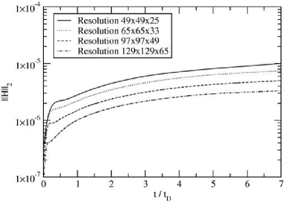
Figure 1: Time evolution of the $L^{2}$ norm of the Hamiltonian constraint for different resolutions (the numbers refer to grid point on a single patch of our mesh refinement grid). The time is normalized to the dynamical timescale $t_{dyn}=R_{e}\sqrt{R_{e}/M}$.

The perturbations applied are both constraint-violating. This is no significant issue, since the discrete evolution of the NOK-BSSN system will introduce constraint violations even if some minimization technique has been applied to the initial data. Fig. 1 shows the evolution of the $L^{2}$ norm of the Hamiltonian constraint for different grid resolutions, for a model perturbed with $\lambda_{i}=\delta_{i1}$ and $B=10^{-3}$. (The time in this figure, and in the subsequent ones, is normalized to $t_{dyn}=R_{e}\sqrt{R_{e}/M}$, where $R_{e}$ is the circumferential equatorial radius, and $M$ is the ADM mass.) Note that, for a typical perturbation amplitude of $\delta\rho/\rho\approx 10^{-3}$, the Hamiltonian constraint will be violated by $\delta H\approx 16\pi\rho\cdot 10^{-3}\approx 2.5\cdot 10^{-7}$, which is sufficiently smaller than the violations during evolution in Fig. 1. Also, tests have been performed where the perturbation amplitude $B$ (cf. eqn. 17) is reduced by a factor of $10$, and found that this does not affect the growth rate of the perturbation, as expected from small perturbations. To conveniently compare different resolutions, the amplitude is kept constant; however, it is possible to reduce the perturbation amplitudes for resolutions significantly higher than the ones used here (specifically, in the regime where $\delta H$ would become comparable to the constraint violations during evolution) to obtain a system where convergence, now to the equilibrium system, does only depend on the well-posedness of the continuum initial-boundary value problem and the stability of the discrete system.

IV.2 The reference polytrope and associated sequences

We start with a polytrope with the same central rest-mass density ($\rho_{c}=3.38\cdot 10^{-6}$) as Saijo’s series of differentially rotating supermassive star models Saijo (2004). To obtain experience with the influence of certain parameters on the stability properties of the relativistic quasi-toroidal polytropes, some sequences containing this reference model have been constructed.

IV.2.1 The reference model

Polytropic index $\Gamma$	$\Gamma$	$4/3$
Central rest-mass density	$\rho_{c}$	$3.38\cdot 10^{-6}$
Degree of differential rotation	$A$	$1/3$
Coordinate axis ratio	$r_{p}/r_{e}$	$0.24$
Density ratio	$\rho_{max}/\rho_{c}$	$16.71$
ADM mass	$M$	$7.003$
Rest mass	$M_{0}$	$7.052$
Equatorial inverse compactness	$R_{e}/M$	$11.71$
Angular momentum	$J$	$52.20$
Normalized angular momentum	$J/M^{2}$	$1.064$
Kinetic over binding energy	$T/|W|$	$0.227$
(See caption)	$\Omega_{e}/\Omega_{K}$	$0.467$

Table 1: Parameters and integral quantities of the reference quasi-toroidal polytrope Zink et al. (2006a). The quantities $\Gamma$, $\rho_{c}$, $A$ and $r_{p}/r_{e}$ are parameters. The quantity $\Omega_{e}$ is the angular velocity on the equator, while $\Omega_{K}$ is the associated Keplerian velocity of the same model. Therefore, the mass-shedding sequence is located at $\Omega_{e}/\Omega_{K}=1$.

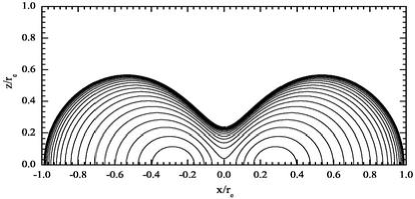
Figure 2: Decadic logarithm of the density in a meridional plane of the model constructed with the parameters in Table 1. The model is of quasi-toroidal nature. Note that this contour plot is included to demonstrate the qualitative properties of the initial model. Therefore, no detailed scale is provided.

The reference model is identical to the model used in Zink et al. (2006a); its parameters and integral quantities are shown in Table 1. Fig. 2 is a graph of the density in the meridional plane for this model. This model has been found to be unstable to perturbations with $m=1$ and $m=2$ (see below, and Zink et al. (2006a)), which lead to fragmentation. In the case of $m=1$, black hole formation has been demonstrated by locating an apparent horizon centered on the fragment Zink et al. (2006a).

IV.2.2 The sequence of axis ratios

Model	$\rho_{c}$	$r_{p}/r_{e}$	$\rho_{max}/\rho_{c}$	$M$	$M_{0}$	$R_{e}/M$	$J$	$J/M^{2}$	$T/|W|$	$\Omega_{e}/\Omega_{K}$
R0.20	$3.38\cdot 10^{-6}$	$0.20$	$38.12$	$6.181$	$6.200$	$9.660$	$38.59$	$1.010$	$0.235$	$0.487$
R0.22	$3.38\cdot 10^{-6}$	$0.22$	$25.69$	$6.662$	$6.710$	$10.41$	$45.46$	$1.024$	$0.228$	$0.475$
R0.24	$3.38\cdot 10^{-6}$	$0.24$	$16.76$	$6.989$	$7.037$	$11.71$	$52.00$	$1.065$	$0.227$	$0.467$
R0.26	$3.38\cdot 10^{-6}$	$0.26$	$11.07$	$7.334$	$7.391$	$13.10$	$58.99$	$1.097$	$0.223$	$0.460$
R0.28	$3.38\cdot 10^{-6}$	$0.28$	$7.312$	$7.585$	$7.646$	$14.83$	$65.19$	$1.133$	$0.219$	$0.455$
R0.30	$3.38\cdot 10^{-6}$	$0.30$	$4.733$	$7.764$	$7.825$	$17.13$	$70.82$	$1.175$	$0.213$	$0.452$
R0.32	$3.38\cdot 10^{-6}$	$0.32$	$2.934$	$7.847$	$7.905$	$20.46$	$75.48$	$1.226$	$0.207$	$0.452$
R0.34	$3.38\cdot 10^{-6}$	$0.34$	$1.539$	$7.755$	$7.803$	$27.42$	$78.72$	$1.309$	$0.196$	$0.463$

Table 2: Parameters and integral quantities of the R sequence of axis ratios, which contains the reference model for $r_{p}/r_{e}=0.24$. Each member of the sequence is denoted by the term R<$r_{p}/r_{e}$>. All models have $\Gamma=4/3$ and $A=1/3$.

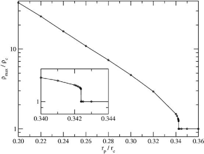
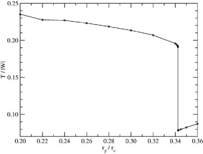
Figure 3: $\rho_{max}/\rho_{c}$ (top) and $T/|W|$ (bottom) for the R sequence. Beyond an axis ratio of $r_{p}/r_{e}\approx 0.3423$, the initial data solver converges to spheroidal models.

A number of sequences containing this model have been constructed to study the stability properties when varying typical parameters. The first of these sequences is parameterized by the coordinate axis ratio $r_{p}/r_{e}$. Its members are denoted by R<$r_{p}/r_{e}$>, and their properties can be found in Table 2. It is apparent that, with increasing axis ratios, the quantity $T/|W|$ and the ratio of maximal to central rest-mass density $\rho_{max}/\rho_{c}$ both decrease monotonically. None of the sequence members is close to the mass-shedding limit. Below $r_{p}/r_{e}=0.20$, no models could be constructed due to failure of convergence. We will also not consider models with larger $r_{p}/r_{e}$. The reason for this is indicated in Fig. 3: Beyond an axis ratio of $r_{p}/r_{e}\approx 0.3423$, quasi-toroidal models could not be constructed as the numerical code fails to converge.

IV.2.3 The sequence of stiffnesses

Model	$\Gamma$	$\rho_{c}$	$\rho_{max}/\rho_{c}$	$M$	$M_{0}$	$R_{e}/M$	$J$	$J/M^{2}$	$T/|W|$	$\Omega_{e}/\Omega_{K}$
G1.333	$4/3$	$3.38\cdot 10^{-6}$	$16.76$	$6.989$	$7.037$	$11.71$	$52.00$	$1.065$	$0.227$	$0.467$
G1.4	$1.4$	$1.32\cdot 10^{-5}$	$16.44$	$2.805$	$2.856$	$11.69$	$8.337$	$1.059$	$0.211$	$0.424$
G1.45	$1.45$	$3.7\cdot 10^{-5}$	$13.83$	$1.624$	$1.662$	$11.70$	$2.767$	$1.049$	$0.202$	$0.404$
G1.5	$1.5$	$9.2\cdot 10^{-5}$	$11.53$	$1.038$	$1.066$	$11.65$	$1.115$	$1.035$	$0.194$	$0.390$
G1.6	$1.6$	$3.75\cdot 10^{-4}$	$8.349$	$0.5197$	$0.5363$	$11.80$	$0.2758$	$1.021$	$0.183$	$0.370$
G2.0	$2.0$	$8.2\cdot 10^{-3}$	$3.880$	$0.1270$	$0.1323$	$11.69$	$0.0155$	$0.9633$	$0.159$	$0.331$

Table 3: Parameters and integral quantities of the G sequence of polytropic coefficient $\Gamma$, which contains the reference model for $\Gamma=4/3$. Each member of the sequence is denoted by the term G<$\Gamma$>. The central density is adjusted to yield approximately the same inverse equatorial compactness $R_{e}/M$ as in the reference model. The models G1.7 to G1.9 have not been constructed, since the models G1.6 and G2.0 were found to be stable. All models have $A=1/3$ and $r_{p}/r_{e}=0.24$.

This sequence is a variation of the parameter $\Gamma$ in the polytropic relation $P=K\rho^{\Gamma}$, which also determines the stiffness of the ideal fluid equation of state $P=(\Gamma-1)\rho\epsilon$ used for evolution. To obtain a sequence of comparable compactness, we adjust the central density $\rho_{c}$ to yield approximately the same $R_{e}/M$. The parameters and integral quantities are shown in Table 3. Along the sequence of increasing $\Gamma$, the value $T/|W|$ decreases from $0.227$ to $0.159$. Therefore, it would also be interesting to consider a sequence of models with varying $\Gamma$, but constant $T/|W|$, by adjusting the axis ratio $r_{p}/r_{e}$ accordingly. Unfortunately, such a sequence could not be obtained, since the initial data solver did not converge to models with the required (low) axis ratios.

IV.2.4 The sequence of compactnesses

Model	$\rho_{c}$	$r_{p}/r_{e}$	$\rho_{max}/\rho_{c}$	$M$	$M_{0}$	$R_{e}/M$	$J$	$J/M^{2}$	$T/|W|$	$\Omega_{e}/\Omega_{K}$
C1	$3.38\cdot 10^{-6}$	$0.24$	$16.76$	$6.989$	$7.037$	$11.71$	$52.00$	$1.065$	$0.227$	$0.467$
C2	$1\cdot 10^{-7}$	$0.24$	$31.06$	$10.65$	$10.74$	$22.72$	$167.0$	$1.474$	$0.225$	$0.434$
C4	$7.5\cdot 10^{-9}$	$0.24$	$37.01$	$12.54$	$12.60$	$45.65$	$326.0$	$2.073$	$0.225$	$0.423$
C8	$8\cdot 10^{-10}$	$0.24$	$39.64$	$13.47$	$13.51$	$89.91$	$525.6$	$2.897$	$0.225$	$0.419$

Table 4: Parameters and integral quantities of the C sequence of compactnesses, which contains the reference model for $\rho_{c}=3.38\cdot 10^{-6}$. Each member of the sequence is denoted by the term C<$a$>, where $a$ denotes the approximate ratio of $R_{e}/M$ to $(R_{e}/M)_{ref}$ of the reference model C1. The sequence is obtained by varying the central rest-mass density. All models have $\Gamma=4/3$ and $A=1/3$.

The next sequence is a variation of the central rest-mass density $\rho_{c}$ while leaving all other parameters fixed. The resulting sequence, as is apparent from Table 4, is also a sequence of inverse equatorial compactnesses $R_{e}/M$. The members have been selected to represent models which are half to one eighth as compact as the reference polytrope. The sequence shows that $T/|W|$ is only slightly affected by the choice of $\rho_{c}$, but $R_{e}/M$ and $J/M^{2}$ change significantly.

IV.3 Quasi-toroidal and spheroidal models of constant central rest-mass density

In addition to sequences containing the reference model, we explore a more extended part of the parameter space of models. We use $\Gamma=4/3$ and $\rho_{c}=10^{-7}$ to define a surface in the parameter space spanned by the axis ratio $r_{p}/r_{e}$ and the degree of differential rotation $A$. While an ideal fluid with $\Gamma=4/3$ is an approximation for the material properties of radiation-pressure dominated stars, the restriction to $\rho_{c}=10^{-7}$ is arbitrary. However, as discussed in Section V, the non-axisymmetric stability of the quasi-toroidal models is probably less sensitive to $\rho_{c}$ than to $r_{p}/r_{e}$ or $A$. The restriction to a plane is necessary since three-dimensional simulations of quasi-toroidal relativistic stars are still expensive; however, selected models will also be studied with different $\rho_{c}$ in Section V.

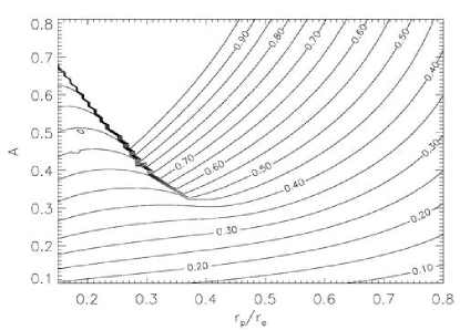
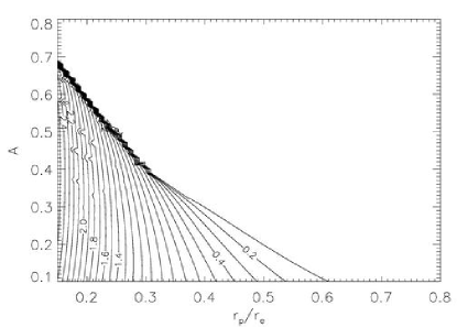
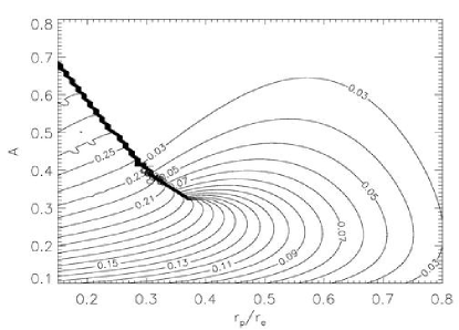
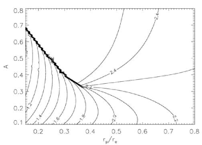
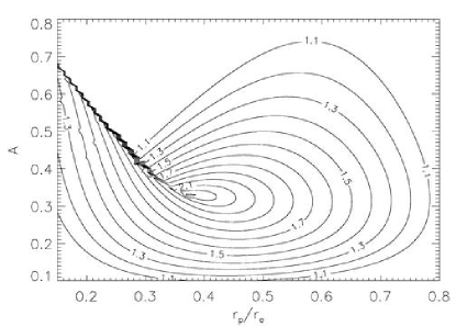
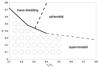
Figure 4: Polytropic models constructed with the RNS code. The plots show the parameter plane spanned by the axis ratio $r_{p}/r_{e}$ and the differential rotation parameter $A$, constrained by $\rho_{c}=10^{-7}$ and $\Gamma=4/3$, and resolved by construction of $6400$ ($80\times 80$) models. Top left: contours of the equatorial stellar over Keplerian angular velocity $\Omega_{e}/\Omega_{K}$ (the mass shedding limit is the isosurface $\Omega_{e}/\Omega_{K}=1$). Top right: decadic logarithm of the ratio of maximal over central density $log_{10}(\rho_{max}/\rho_{c})$. Middle left: rotation parameter $T/|W|$. Middle right: decadic logarithm of the inverse equatorial compactness $R_{e}/M$. Bottom left: normalized angular momentum $J/M^{2}$. Bottom right: Selection of evolved initial models. The thick continuous line marks the jump between quasi-toroidal and spheroidal models apparent in the top left to bottom left plots, the thick dashed line is the mass-shedding limit, and the thin dashed line indicates an approximate division between spheroidal and quasi-toroidal models. The models selected for numerical evolution are marked by circles.

Model	$\rho_{c}$	$A$	$r_{p}/r_{e}$	$\rho_{max}/\rho_{c}$	$M$	$M_{0}$	$R_{e}/M$	$J$	$J/M^{2}$	$T/|W|$	$\Omega_{e}/\Omega_{K}$
A0.1R0.15	$10^{-7}$	$0.1$	$0.15$	$246.8$	$4.896$	$4.893$	$20.82$	$18.62$	$0.777$	$0.124$	$0.195$
A0.1R0.50	$10^{-7}$	$0.1$	$0.5$	$1.881$	$5.387$	$5.390$	$106.2$	$31.69$	$1.092$	$0.0706$	$0.126$
A0.3R0.15	$10^{-7}$	$0.3$	$0.15$	$356.9$	$7.964$	$8.034$	$12.04$	$70.66$	$1.114$	$0.228$	$0.434$
A0.3R0.50	$10^{-7}$	$0.3$	$0.5$	$1.00005$	$6.291$	$6.300$	$151.4$	$77.10$	$1.948$	$0.108$	$0.360$
A0.6R0.15	$10^{-7}$	$0.6$	$0.15$	$541.2$	$21.29$	$21.39$	$61.62$	$1360$	$3.000$	$0.276$	$0.650$

Table 5: Parameters and integral quantities of selected quasi-toroidal models in the parameter space plane defined by $\rho_{c}=10^{-7}$ and $\Gamma=4/3$. The models are labelled by A<$A$>R<$r_{p}/r_{e}$>. All models have $\Gamma=4/3$.

The general properties of the polytropes obtained with the RNS code is shown for a central rest-mass density $\rho_{c}=10^{-7}$ in Fig. 4. The top left plot shows the function $\Omega_{e}/\Omega_{K}$, where $\Omega_{e}$ is the equatorial stellar angular velocity, and $\Omega_{K}$ is the corresponding Keplerian angular velocity. The jump indicated in the equilibrium model surface has already been found in the R sequence, see Fig. 3.

The topological nature of the polytropes is shown in the top right panel of Fig. 4, which plots the ratio of maximal to central rest-mass density $\rho_{max}/\rho_{c}$. This value measures the degree of toroidal deformation of the model, with the limiting cases $\rho_{max}/\rho_{c}=1$ (purely spheroidal polytrope) and $\rho_{max}/\rho_{c}=\infty$ (purely toroidal polytrope). Since we are interested in the properties of quasi-toroidal models, we will concentrate our study on the part of this plot covered by contour lines.

Judging from the study of Newtonian polytropes, one would expect that the function $T/|W|$ is related to non-axisymmetric stability. For the sequence of Maclaurin spheroids, the dynamically unstable subset can be described by the simple inequality $T/|W|\geq(T/|W|)_{dyn}$ Chandrasekhar (1969), suggesting to use $T/|W|$ to parameterize the sequence. While the situation is clearly more complicated with relativistic, differentially rotating polytropic models, the middle left plot in Fig. 4 suggests that the quasi-toroidal models with small axis ratio $r_{p}/r_{e}=0.15$ are more likely to be unstable to non-axisymmetric perturbations. We will study this in Section V.

The bottom right panel in Fig. 4 is an illustration of the initial model parameter space. The polytropes which have been evolved numerically are marked by circles. The equilibrium parameters and associated quantities of a selected set of these polytropes are listed in Table 5.

IV.4 A sequence of central rest-mass densities containing the model A0.2R0.40

Model	$\Gamma$	$\rho_{c}$	$A$	$r_{p}/r_{e}$	$\rho_{max}/\rho_{c}$	$M$	$M_{0}$	$R_{e}/M$	$J$	$J/M^{2}$	$T/|W|$	$\Omega_{e}/\Omega_{K}$
L1	$4/3$	$10^{-4}$	$0.2$	$0.354$	$1.874$	$3.621$	$3.578$	$14.85$	$9.952$	$0.760$	$0.144$	$0.301$
L2	$4/3$	$10^{-5}$	$0.2$	$0.378$	$2.434$	$5.173$	$5.177$	$20.67$	$24.06$	$0.900$	$0.144$	$0.280$
L3	$4/3$	$10^{-6}$	$0.2$	$0.392$	$2.644$	$6.505$	$6.524$	$35.69$	$49.51$	$1.170$	$0.144$	$0.269$
L4	$4/3$	$10^{-7}$	$0.2$	$0.4$	$2.689$	$7.348$	$7.362$	$69.41$	$87.33$	$1.617$	$0.144$	$0.264$

Table 6: Parameters and integral quantities of the L sequence. This sequence is constructed by starting from the model A0.2R0.40 (cf. Section IV.3), which is identical to the model L4, and keeping $T/|W|$ fixed while reducing the central density.

The L sequence (see Table 6) is a variation of the C sequence in Section IV.2.4. It starts from the model A0.2R0.40 instead of the reference model. In contrast to the C sequence, we do not keep the axis ratio $r_{p}/r_{e}$ fixed while varying the central rest-mass density, but rather the quantity $T/|W|$. This sequence is constructed to study the influence of the compactness on a model near the boundary to the region denoted by “I” in Fig. 25 (see also Section V.8).

V Results

The models constructed in Section IV have been evolved numerically to study their stability properties. We will start with discussing the reference model, and show that it is unstable to a non-axisymmetric perturbation which leads to black hole formation. Then, the sequences of axis ratios, compactness and stiffness from Section IV are studied. Finally, the parameter plane constrained by $\Gamma=4/3$ and $\rho_{c}=10^{-7}$ is sampled, and the coordinate location of the corotation point on a sequence in this plane is investigated.

V.1 Evolution of the reference model

The main results from evolving the reference polytrope defined in Section IV.2.2 have already been discussed in Zink et al. (2006a). When subject to a perturbation of the form given in eqn. 17, the torus transforms into one ($m=1$) or two ($m=2$) fragments. In the case of the $m=1$ perturbation, it has been shown that the fragment is partially covered by an apparent horizon, indicating black hole formation.

In this section, we will take a more detailed look at this model, and discuss some technical issues relevant to the parameter space study below.

V.1.1 Development of the instability

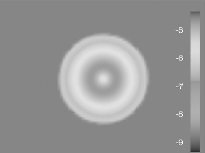
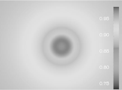
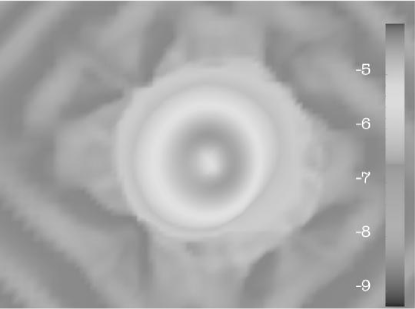
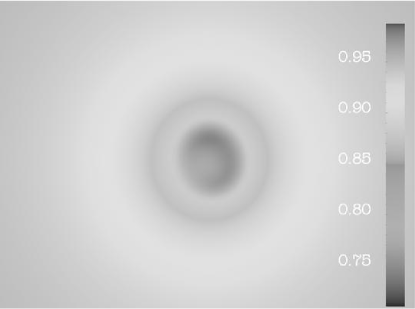
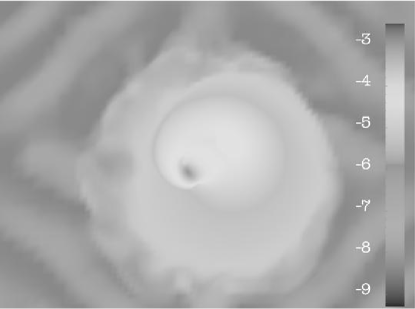
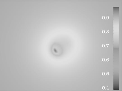
Figure 5: Development of the fragmentation instability in the reference polytrope. The left sequence of plots show the decadic logarithm of rest-mass density in the equatorial plane, the right sequence of plots shows the lapse function. The snapshots correspond to times $t/t_{dyn}=0$ (top), $6.28$ (middle) and $7.48$ (bottom). The initial model, perturbed by eqn. 17 with $\lambda_{m}=1$ for $m=1,\ldots,4$, develops a spiral arm instability and a collapsing fragment. The domain outside the star initially has the density of the artificial atmosphere ($\rho_{atm}\approx 5\cdot 10^{-10}$), and the artifacts outside the star are caused by interactions of the atmosphere with the stellar surface and the outer boundaries of the computational domain. Here, and in all evolution sequences which follow, the extent of the spatial coordinate domain plotted is the same in all snapshots. Also, note that the color map is adapted to the range of function values in each plot.

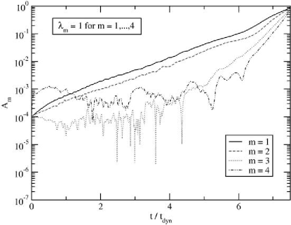
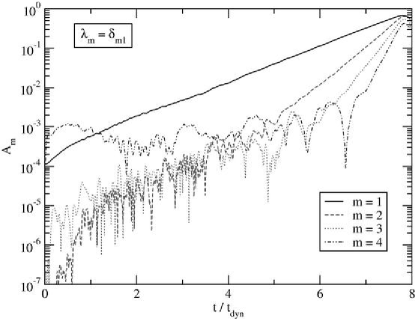
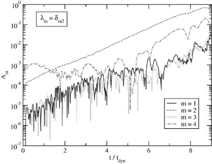
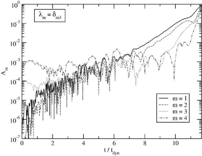
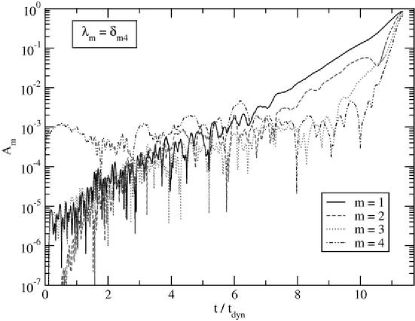
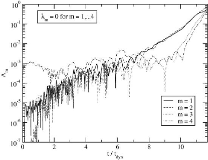
Figure 6: Mode amplitudes versus time, extracted at $r=0.25R_{e}$, the radius of highest rest-mass density in the initial model, for different initial perturbations. The amplitude $A_{m}$ is the $m$-th harmonic Fourier projection of the density, normalized to the average value. The perturbations corresponding to each plot are (cf. also eqn. 17): $\lambda_{m}=1$ for $m=1,\ldots,4$ (top left), $\lambda_{m}=\delta_{m1}$ (top right), $\lambda_{m}=\delta_{m2}$ (middle left), $\lambda_{m}=\delta_{m3}$ (middle right), $\lambda_{m}=\delta_{m4}$ (bottom left), and $\lambda_{m}=0$ for $m=1,\ldots,4$. For details see text.

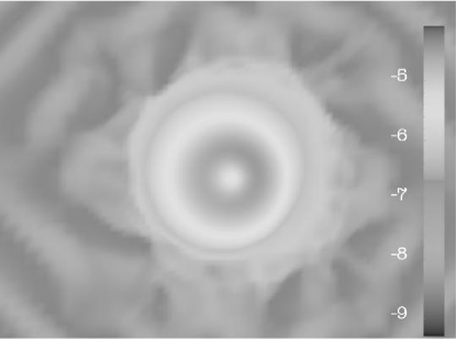
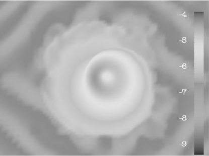
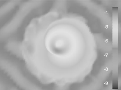
Figure 7: Similar to Fig. 5, but now for a perturbation $\lambda_{m}=\delta_{m1}$. Shown is the decadic logarithm of the density in the equatorial plane. The snapshots correspond to times $t/t_{dyn}=6.28$ (top), $7.11$ (middle) and $7.48$ (bottom). While the $m=2$ mode is now suppressed, the qualitative evolution is similar to that displayed in Fig. 5.

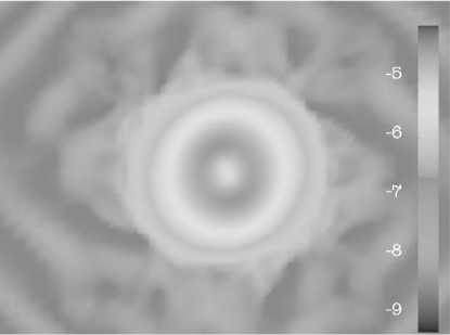
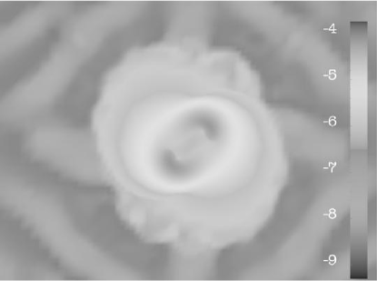
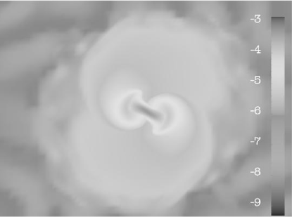
c

Figure 8: Similar to Fig. 5, but for a perturbation $\lambda_{m}=\delta_{m2}$. Shown is the decadic logarithm of the density in the equatorial plane. The snapshots correspond to times $t/t_{dyn}=6.28$ (top), $7.66$ (middle) and $8.85$ (bottom). Two fragments develop and encounter a runaway instability while orbiting each other.

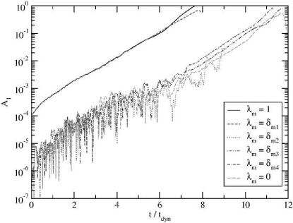
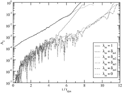
Figure 9: Comparison of mode amplitude versus time for different initial perturbations. The upper panel shows the mode amplitude $A_{1}$, and the lower one shows $A_{2}$. Note that, in the case $\lambda_{m}=\delta_{m1}$, the $m=2$ mode is dominated by non-linear effects from the fragmentation.

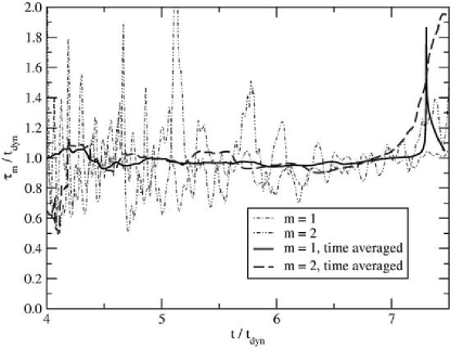
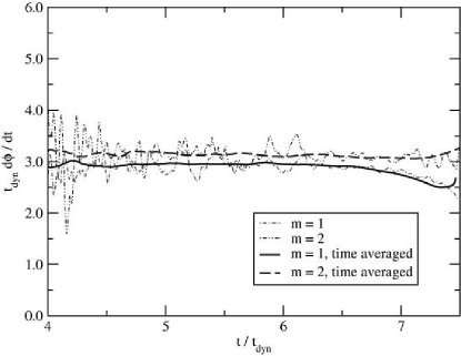
Figure 10: Local growth times $\tau_{m}(t):=(d\ln A/dt)^{-1}$ (top) and frequencies $d\phi_{m}/dt$ (bottom) for modes $m=1$ and $m=2$, both taken from simulations with the corresponding initial perturbation. The plots denoted by “time averaged” are running averages over $t_{dyn}$.

Fig. 5 shows the development of the non-axisymmetric instability in the equatorial plane when using a perturbation of the form given by eqn. 17 and $\lambda_{m}=1$ for $m=1,\ldots,4$. The density perturbation is not apparent in the initial model, but, after a few dynamical timescales, an instability has developed which entirely destroys the structure of the star. (Note that the artifacts outside the stellar surface are caused by the introduction of an artifical atmosphere.) In this case, one collapsing off-center fragment forms in the system. Judging from Fig. 5 there is a “collapse of the lapse,” which is a well-known effect when using singularity-avoiding slicings, and which indicates the development of a black hole.

To investigate the instability more closely, the Fourier mode extraction discussed in Section III has been applied to the coordinate radius of highest density in the initial model, which is at $r=0.25R_{e}$. We concentrate on this radius for reasons already discussed: different extraction radii will be considered in Section V.1.2. The top left panel of Fig. 6 displays the evolution of the amplitude of the first four Fourier modes $A_{m}$, $m=1,\ldots,4$, in this evolution. Although all four modes have been injected with the same amplitude ($\approx 10^{-4}$), the $m=4$ mode displays a significant initial growth of about an order of magnitude, and then oscillates around this level until $t/t_{dyn}\approx 6$, where non-linear effects become important. The high level of $m=4$ noise is very likely an artefact of the Cartesian grids used for the simulation. Support for this argument can be obtained by considering that the equatorial section of the grid has a discrete $C_{4}$ symmetry, and by comparing Fig. 3 and 4 in Centrella et al. (2001), where results from the development of a similar non-axisymmetric instability, though in Newtonian gravity, were achieved on cylindrical and Cartesian grids. We note that the discrete model appears to be stable against this perturbation, and also against the $m=3$ perturbation. The remaining modes are unstable, and the growth times of both modes are similar. In this specific case the $m=1$ structure dominates the late-time evolution, and leads to the spiral arm structure and fragmentation visible in Fig. 5.

The structure of the numerical noise depends on the grid geometry, resolution, finite difference operators and discrete methods for treating hydrodynamics, the outer boundary conditions and the artificial atmosphere. Therefore, it is important to know to which degree the four Fourier modes are coupled during the evolution. Since the initial perturbation is considered to be “small,” which holds when compared to the $m=4$ numerical noise level discussed above, we expect that coupling becomes important as soon as the amplitudes $A_{m}$ get close to unity. To determine this in the reference model, a number of simulations have been performed with perturbations of the form given by eqn. 17, but with $\lambda_{m}=\delta_{mj}$ for different $j\in\{1,\ldots,4\}$ to select individual modes, and one simulation where no perturbation is applied. The mode amplitudes in these simulations are shown in Fig. 6, and the $m=1$ and $m=2$ modes are compared to the perturbation with $\lambda_{m}=1$ in Fig. 9. As long as the mode development is not dominated by another mode which at a higher amplitude, e.g. as in the case of the $m=2$ mode in the top right panel in Fig. 6, the growth times are comparable for different perturbations.

The high-amplitude, strongly non-linear development at late times is sensitive to the perturbation function, as is visible from the evolutions shown in Fig. 7 and 8. In the case of the $m=1$ perturbation, a single fragment develops and collapses in a similar manner to the case $\lambda_{m}=1$. With an $m=2$ perturbation, however, two orbiting fragments develop, contract, and subsequently encounter a runaway instability in the center (bottom right panel in Fig. 8). Any perturbation with different values for $\lambda_{1}$ and $\lambda_{2}$ might produce a mixture of this spiral arm and binary-system fragmentation instability. One might argue that a fine-grained parameter space study in the space of $\lambda_{1}$ and $\lambda_{2}$ is necessary to obtain a more complete understanding of the remnants. However, the reference polytrope is already well inside the unstable region of the parameter space. We will see in Section V.5 that, on a sequence of increasing $T/|W|$, the $m=1$ mode dominates first. As has been shown in Zink et al. (2006a), this process of fragmentation is black-hole forming. Unfortunately, around the time of horizon formation the evolution fails. This appears to be due to the growth of small scale features that cannot be adequately resolved leading to unphysical oscillations. It seems possible that a more robust gauge condition, artificial dissipation Baiotti and Rezzolla (2006) or excision techniques Lehner et al. (2005); Zink et al. (2006b) could avoid these problems.

To investigate the growth time $\tau$ of the modes, which, in the context of linear theory, is defined by the relation $A_{m}(t)=A_{m}(t=0)\exp(t/\tau_{m})$, we plot the function $\tau_{m}(t):=(d\ln A/dt)^{-1}$ in the top panel of Fig. 10 for $m=1$ and $m=2$, using different initial perturbations of the reference polytrope as before. As expected for a dynamical instability, the growth times are of the order of the dynamical timescale. Finally, in the bottom panel of Fig. 10 the mode frequencies $\omega_{m}(t)=d\phi_{m}/dt$ (as extracted from the Fourier decomposition of the density on a the coordinate radius of highest initial density) are plotted versus time. These, and the connected pattern speeds $\omega/m$, will be important in the discussion of the corotation band in Section V.1.3.

V.1.2 Some results on the global nature of the instability

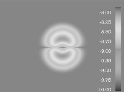
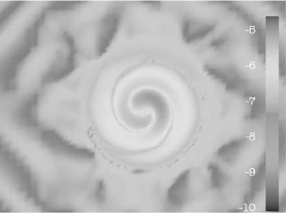
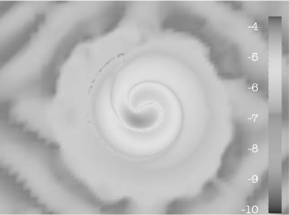
Figure 11: Contour plot of the function $\log_{10}(|\rho(x,y,z,t)-\rho_{0}(x,y,z)|+\epsilon)$ in the equatorial plane, where $\rho$ denotes the rest-mass density of the $m=1$ evolution shown in Fig. 7, $\rho_{0}$ denotes the the density function of the equilibrium polytrope, and $\epsilon$ is a small number ($\epsilon=10^{-10}$ in this plot).

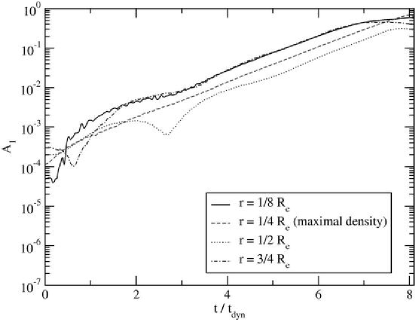
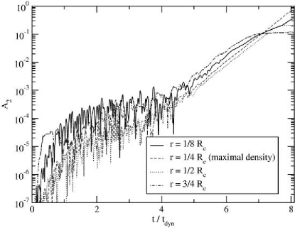
Figure 12: Evolution of the mode amplitudes $A_{1}$ and $A_{2}$ in the reference polytrope perturbed by $\lambda_{m}=\delta_{m1}$, for different mode extraction radii. The radius of highest initial density is indicated.

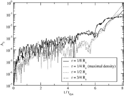
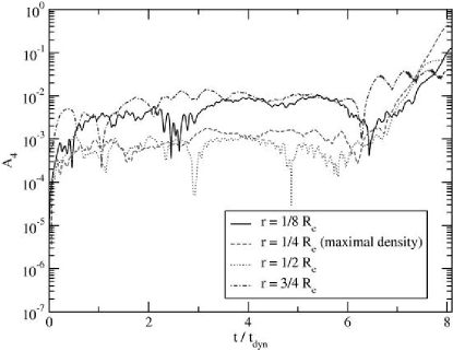
Figure 13: Same as Fig. 12, but for the mode amplitudes $A_{3}$ and $A_{4}$.

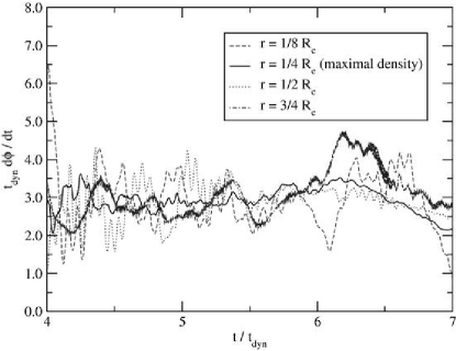
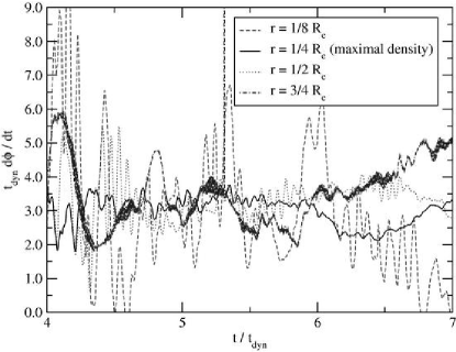
Figure 14: Local mode frequency $t_{dyn}d\phi/dt$ for the modes $m=1$ (top) and $m=2$ (bottom) in the reference polytrope, extracted at different radii in the equatorial plane.

While we do not focus on the global nature of the quasi-normal modes of general relativistic quasi-toroidal polytropes here, this section will give some indication about the structure of the instability. Consider Fig. 11 which displays the equatorial distribution of the function $\log_{10}(|\rho(x,y,z,t)-\rho_{0}(x,y,z)|+\epsilon)$, where $\rho_{0}$ is the density function of the equilibrium polytrope and $\epsilon=10^{-10}$. These logarithmic difference plots exhibit the node lines of the unstable mode corresponding to $m=1$ in the equatorial plane, and show the spiral-arm structure of the fragmentation instability.

The mode amplitudes at different extraction radii in the equatorial plane are shown, for a perturbation with $\lambda_{m}=\delta_{m1}$, in Fig. 12 and 13. The development of the unstable modes is not very sensitive to the extraction radius, at least as long as the amplitude of the dominant mode is not close to unity. Fig. 14 suggests that the local mode frequency does not depend strongly on the radius, at least within the considerable uncertainties of the plot.

V.1.3 The location of the unstable modes in the corotation band

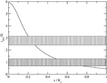
Figure 15: Angular velocity of the reference polytrope over the $x$ axis (black line), and approximate location (with error bar) of the pattern speed of the $m=1$ mode (upper rectangle), and the $m=2$ mode (lower rectangle). Both modes are inside the corotation band.

To determine the location of the instability with respect to the corotation band, we define a coordinate angular velocity of the initial model by

$$\Omega(\varpi)\equiv\alpha v^{\phi}-\beta^{\phi}.$$ (18)

This can be compared to the mode pattern speed $1/m\,d\phi/dt$, which we will assume to be valid for the whole star (cf. Fig. 14), to determine whether a certain mode has a corotation point. In Fig. 15, the angular velocity is plotted in addition to the numerical approximation of the location of the $m=1$ and $m=2$ pattern speeds. We find that both modes have corotation points: the $m=1$ mode near the radius of highest density at $0.25\,R_{e}$, and the $m=2$ mode near $0.5\ldots 0.6\,R_{e}$.

V.1.4 Grid resolution and convergence

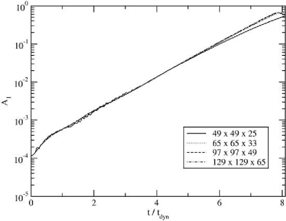
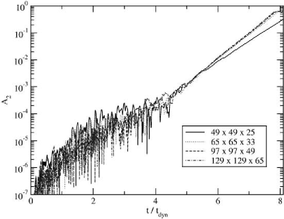
Figure 16: Evolution of the mode amplitudes $A_{1}$ (top) and $A_{2}$ (bottom) for different grid resolutions. The grid sizes in the legend refer to the four outer grid patches; the innermost patch covering the high-density central toroidal region of the star has a resolution of $65\times 65\times 33$, $97\times 97\times 49$, $129\times 129\times 65$ or $193\times 193\times 97$, correspondingly.

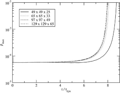
Figure 17: Same as Fig. 16, but for the evolution of the maximum of the rest-mass density $\rho_{max}$.

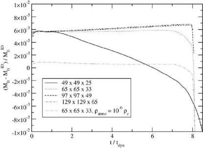
Figure 18: Same as Fig. 16, but for the evolution of the total rest mass $M_{0}$. The values are normalized to the initial rest mass ${M_{0}}^{ID}$ obtained from the initial data solver. The last graph is from a simulation with a less dense artificial atmosphere.

For any parameter study with numerical methods, it is important to have an understanding of the amount of grid resolution needed to extract the physical features under consideration. A typical way to gauge this is to evolve a system with different resolutions and to compare the results. For the black-hole forming fragmentation instability shown in Section V.1.1, it is expected that different phases of the evolution have substantially different resolution requirements. During the nearly exponential growth of the instability at low amplitudes (which we will call linear regime), the equilibrium structure of the star as a whole needs to be covered appropriately. The instability is, at first, a low-frequency effect on the star, and as such it is not expected to dominate the resolution requirements. However, if the fragment evolves into a black hole (in the non-linear regime), it needs to be resolved with significantly more grid points.

As explained in Section III, the star is covered by a grid with fixed mesh refinement. Typically, five grid patches are used, centered on each other, and with an increase of resolution by a factor 2 each. Only the central patch with highest resolution, which covers the region of highest density, is 0.75 times as extended as the second finest one to reduce artefacts from inter-patch boundaries. To test convergence, the reference model has been evolved with $49\times 49\times 25$ (grid spacing $h\approx 0.29M$), $65\times 65\times 33$ ($h\approx 0.22M$), $97\times 97\times 49$ ($h\approx 0.15M$) and $129\times 129\times 65$ ($h\approx 0.11M$) zones per outer grid patch; the innermost patch covering the high-density toroidal region has $65\times 65\times 33$, $97\times 97\times 49$, $129\times 129\times 65$ or $193\times 193\times 97$ grid zones. Also, the initial data was calculated with a grid of $401\times 201$, $601\times 301$, $1201\times 601$ and $2401\times 1201$ zones.

The results from evolving the reference model with an $m=1$ perturbation at different resolutions are shown in Figs. 1, 16, 17 and 18. The convergence of the Hamiltonian constraint has already been discussed in Section IV.1. The time development of the mode amplitudes has a noticeably different growth only at the lowest resolution. The evolution of the maximum of the rest-mass density (Fig. 17) exhibits a similar behaviour. Finally, the total rest mass of the system is conserved from within $1.4\%$ (lowest resolution) to $0.1\%$ (higher resolutions). The drift in the rest-mass can be explained by our use of an artificial atmosphere: The rest-mass density of the atmosphere is $10^{-5}\rho_{c}=3.38\cdot 10^{-11}$, which corresponds to an approximate total mass of $M_{0,atmo}\approx 3.8\cdot 10^{-3}$ in a domain of coordinate volume $1040^{3}$ (not taking into account the volume form). This translates into a systematic shift in the total rest mass of the system as apparent when comparing to an evolution with a lower atmospheric density (bottom panel in Fig. 18), and a drift caused by the intrinsic atmospheric dynamics and the interaction with the outer boundary. Note that this is to be considered a (non-sharp) upper limit on the systematic errors induced by the atmosphere, because one could always extend the total computational domain arbitrarily without affecting the core region significantly.

Judging from the resolution study in Figs. 1, 16, 17 and 18, we think that the lowest resolution considered here (which already covers the equatorial radius of the star with about 60 grid points when comparing to uniform grids) is sufficient to get qualitatively correct results. Quantitatively, the errors in rest mass are in a range of a few percent. The next highest resolution of $65\times 65\times 33$ ($h\approx 0.22M$) seems accurate to within about one percent. This resolution will therefore be used for the parameter study below. This is reasonable since the structure of the quasi-toroidal models has similar features, and therefore similar requirements concerning resolution. Nevertheless, selected models have been tested for convergence independently from the reference polytrope.

V.1.5 Influence of the artificial atmosphere

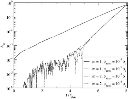
Figure 19: Evolution of the mode amplitudes $A_{1}$ and $A_{2}$ in the reference polytrope, for artificial atmospheres of different density $\rho_{atm}/\rho_{c}$.

The standard artificial atmosphere we employ in our simulations has a density several orders of magnitude lower than the average density in the star, so we expect that it does not influence the dynamical properties of the star significantly. The atmospheric density is set in terms of the central density of the star: we have used a ratio of $10^{-5}$ in most simulations. To test the influence of this parameter, we have evolved the reference model also with a ten times lower atmospheric density (i.e. $10^{-6}\rho_{c}$), and with an $m=1$ perturbation. The results are shown in Fig. 18 and 19. The latter shows that the dominant $m=1$ mode is not influenced by the atmospheric setting, while the $m=2$ amplitude shows dependence on the atmosphere setting only as long as its amplitude is on the level of the numerical noise.

V.2 Evolution of the sequence of axis ratios

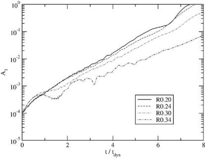
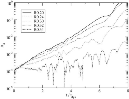
Figure 20: Evolution of the mode amplitudes $A_{1}$ and $A_{2}$ for different members of the R sequence (cf. Table 2).

The R sequence has been described in Section IV.2.2. From Table 2, it is apparent that higher values of $r_{p}/r_{e}$ are connected to lower $T/|W|$. In Maclaurin spheroids, this is related to a stabilization of the initial model. Consider Fig. 20: The growth time of the modes $m=1$ and $m=2$ increases with lower $r_{p}/r_{e}$, which indeed is a sign for approaching a limit of stability.

V.3 Evolution of the sequence of stiffnesses

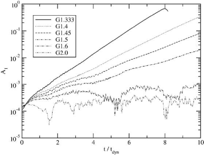
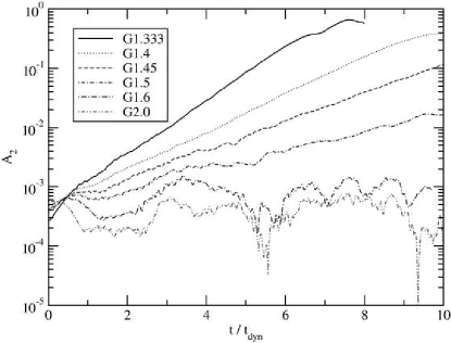
Figure 21: Evolution of the mode amplitudes $A_{1}$ and $A_{2}$ for different members of the G sequence (cf. Table 3).

The change in the instability along the G sequence described in Section IV.2.3 is shown in Fig. 21. With increasing $\Gamma$, and $T/|W|$ decreasing from $0.227$ to $0.159$ (cf. Table 3), both the $m=1$ and the $m=2$ modes are stabilized. The member G2.0 with $\Gamma=2$ is of special interest, since this choice is often used to obtain a simple polytropic equilibrium model of neutron stars. While it is known that strong differential rotation can induce bar-mode instabilities in neutron stars Shibata et al. (2000b); Saijo et al. (2001); Baiotti et al. (2006), the particular model $G2.0$ does not appear to be $m=2$ unstable (note, however, the limitations of our method to determine stability expressed in Section V.7).

V.4 Evolution of the sequence of compactnesses

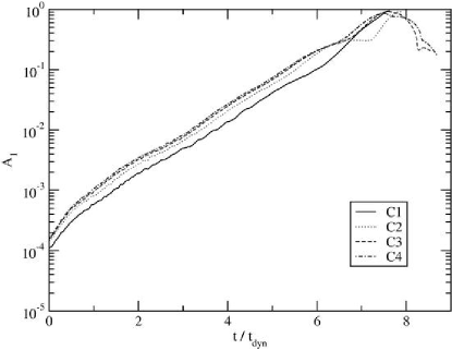
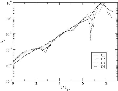
Figure 22: Evolution of the mode amplitudes $A_{1}$ and $A_{2}$ for different members of the C sequence (cf. Table 4).

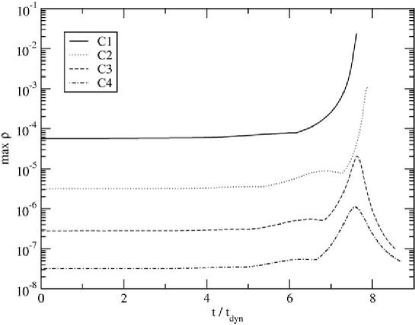
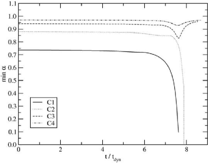
Figure 23: Evolution of the maximum of the rest-mass density $\rho$ and the minimum of the lapse function $\alpha$ for different members of the C sequence.

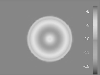
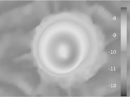
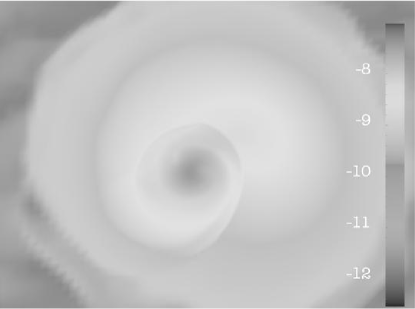
Figure 24: Evolution of density in the equatorial plane of the model C8. Shown is the decadic logarithm of the rest-mass density. The snapshots were taken at times $t/t_{dyn}=0$ (top), $6.28$ (middle) and $8.28$ (bottom). In contrast to the more compact model C1, which is the reference polytrope investigated earlier (cf. Fig. 5), the fragment re-expands after a maximal compression.

The mode amplitudes $A_{1}$ and $A_{2}$ for different members of the C sequence (cf. Section IV.2.4 and Table 4) are shown in Fig. 22. The plot demonstrates that different choices of $\rho_{c}$ do not have a significant effect on the growth time of the mode, which is in contrast to the effects of $\Gamma$ and $r_{p}/r_{e}$ discussed above. However, while the linear development of the mode is similar for different compactnesses, the non-linear behaviour is not. Consider Fig. 23: The reference polytrope C1 and the model C2, which is about half as compact, both show an unbounded growth in the maximum of the density and a collapse of the lapse, indicating black hole formation. The models C4 and C8, however, appear to avoid black hole formation and re-expand after a state of maximum compression. Fig. 24 shows these different types of evolution for the model C8 in more detail: In contrast to the black hole-forming case C1, the fragment re-expands after the collapse in this evolution. This is not unexpected, since the Newtonian limit, for an equation of state $\Gamma=4/3$, admits a stable equilibrium state of the fragment if it has sufficient rotation. We conclude therefore that, even when the growth time of the instability is quite similar for stars of different compactness, the outcome of the fragmentation can differ drastically.

V.5 Evolution of quasi-toroidal models of constant central rest-mass density

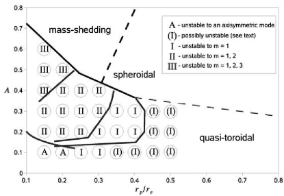
Figure 25: Stability of quasi-toroidal models with $\rho_{c}=10^{-7}$ (cf. Fig. 4). A Latin number denotes the highest azimuthal order of the unstable modes, i.e. “I” for $m=1$ unstable, “II” for $m=1,2$ unstable, and “III” for $m=1,2,3$ unstable. Models denoted by “(I)” are either long-term unstable with growth times $\tau\gg t_{dyn}$, or stable (see text), and models denoted by “A” exhibit an axisymmetric instability. The red line in the lower left is the approximate location of the sequence $J/M^{2}=1$ (cf. Fig. 4), and the three blue lines inside the quasi-toroidal region are the approximate locations of sequences with $T/|W|=0.14$ (right), $T/|W|=0.18$ (middle) and $T/|W|=0.26$ (left).

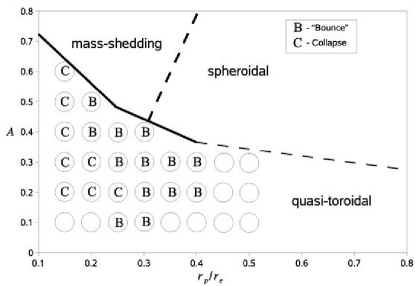
Figure 26: Remnants of the models from Fig. 25, which are unstable with respect to non-axisymmetric modes. The non-linear behaviour has been analyzed by observing the evolution of the function $\min\alpha$ (see also Fig. 23). Models which show a minimum in this function are marked by “B” for “bounce,” while models exhibiting an exponential collapse of the lapse are marked by “C” for “collapse.”

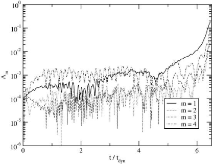
Figure 27: Mode amplitudes in the model A0.1R0.15 (cf. Table 5), extracted at the radius of highest initial rest-mass density.

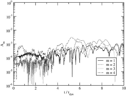
Figure 28: Mode amplitudes in the model A0.1R0.50 (cf. Table 5), extracted at the radius of highest initial rest-mass density.

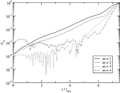
Figure 29: Mode amplitudes in the model A0.3R0.15 (cf. Table 5), extracted at the radius of highest initial rest-mass density.

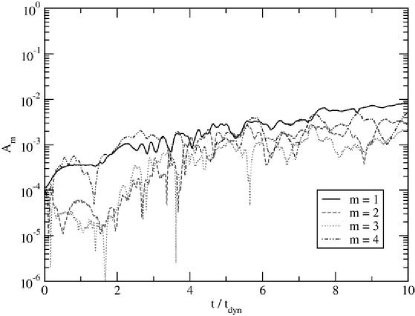
Figure 30: Mode amplitudes in the model A0.3R0.50 (cf. Table 5), extracted at the radius of highest initial rest-mass density.

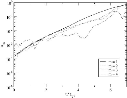
Figure 31: Mode amplitudes in the model A0.6R0.15 (cf. Table 5), extracted at the radius of highest initial rest-mass density.

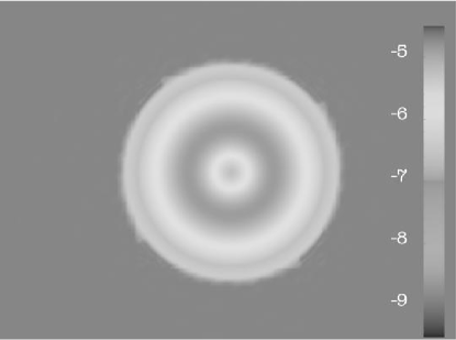
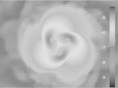
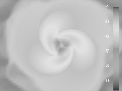
Figure 32: Equatorial density evolution of the model A0.6R0.15, with an $m=3$ perturbation. (Note that, in Fig. 31, a perturbation with $\lambda_{m}=1$ has been used instead). Shown is the decadic logarithm of the rest-mass density. The snapshots were takes at times $t/t_{dyn}=0$ (top), $6.28$ (middle) and $7.60$ (bottom). Three fragments develop and subsequently encounter collapse similar to the two-fragment case (cf. Fig. 8). The evolution of the model perturbed with $m=1$ and $m=2$ is similar to the corresponding one in the reference polytrope.

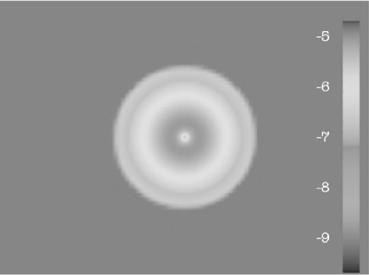
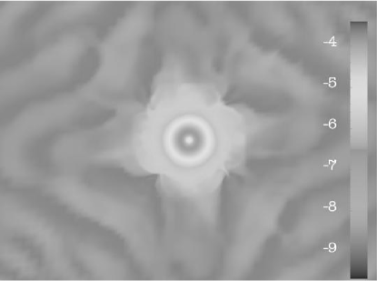
Figure 33: Equatorial density evolution of the model A0.1R0.15. Shown is the decadic logarithm of the rest-mass density. The snapshots were takes at times $t/t_{dyn}=0$ (top) and $6.28$ (bottom). The model exhibits an axisymmetric instability.

The structure of the parameter space plane $\Gamma=4/3$ and $\rho_{c}=10^{-7}$ has been discussed in Section IV.3. As already noted, the necessity of investigating only one plane is determined primarily by the computational cost of three-dimensional general relativistic hydrodynamical simulations. Also, the choice of the central density does not seem to affect the almost exponential development of a non-axisymmetric unstable mode in the linear regime considerably, even for very compact quasi-toroidal polytropes (cf. Section V.4), which is in contrast to axisymmetric modes. Finally, we note that the models with $\rho_{c}=10^{-7}$ are already quite compact, with $R_{e}/M\approx 10\ldots 100$, and $r_{p}/M\approx 2\ldots 70$.

To investigate the stability of these models, the initial data indicated by circles in the bottom right panel of Fig. 4 have been evolved, imposing a perturbation of the form given by eqn. 17 with $\lambda_{m}=1$, and with a resolution of $65\times 65\times 33$ grid points in the outer patches, and $97\times 97\times 49$ in the innermost patch. Selected models have been tested against individual $m=j$ perturbations with $\lambda_{m}=\delta_{mj}$, with different resolutions, and different densities of the artificial atmosphere, to test consistency and convergence. Also, central rest-mass densities different from $10^{-7}$ were investigated in a few models.

Fig. 25 gives an overview of the stability properties of the selected models. The Latin numbers “I” to “III” refer to the highest $m$ with an unstable mode, i.e. in addition to the reference polytrope, which belongs to the class “II,” we find models which are unstable to an $m=3$ perturbation, and models which appear to be stable against $m=2$ (within the restrictions illustrated in Section V.7). The models denoted with an “A” have been found to be unstable to an axisymmetric mode, and collapse before any non-axisymmetric instability develops. Finally, the models marked with “(I)” are either stable or long-term unstable with a growth time $\tau\gg t_{dyn}$. Each model has been evolved for up to $10\,t_{dyn}$ to determine its stability. This limit is arbitrary, but imposed by the significant resource requirements of these simulations. If no mode amplitude exceeds the level of the $m=4$ noise during this time, the model is marked with a “(I).” This does not imply that the model is actually stable, and we will investigate a specific model denoted by “(I)” later. We will find it to be unstable to an $m=1$ mode with slow growth (Section V.7).

The additional lines in Fig. 25 are approximate isolines of the functions $T/|W|$ for the values $0.14$, $0.18$ and $0.26$ and of the function $J/M^{2}$ for the value $1$. As long as the models do not rotate too differentially, $T/|W|$ still seems to be a reasonable indicator of the non-axisymmetric stability of the polytropes, even though they are quasi-toroidal and relativistic.

The nature of the non-linear behaviour of models exhibiting a non-axisymmetric instability is indicated in Fig. 26. We use the evolution of the minimum of the lapse function to classify the models, see also Fig. 23. Models denoted by “B” have a global minimum in the lapse, while models denoted by “C” do not. Given that the compactness of the models increases with smaller axis ratios in this plot (cf. Fig. 4), we expect that a black hole forms for each member of the “C” class. To determine this uniquely, each of these models should be tested using the adaptive mesh-refinement technique presented in Zink et al. (2006a), which is, however, beyond the scope of this study.

In Fig. 27 to 31, we have plotted the mode amplitudes $A_{m}$ for selected models (cf. Table 5). The evolution of the model A0.3R0.15 (Fig. 29) is quite similar to that of the reference polytrope. Model A0.6R0.15 is further inside the unstable region, and exhibits also an $m=3$ instability: the density evolution of this mode is plotted in Fig. 32. The models A0.1R0.50 and A0.3R0.50 are stable within the numerical restrictions mentioned above.

The model A0.1R0.15 seems to have an unusual evolution of the mode amplitudes; this also applies to the model A0.1R0.20, which is not shown here. The density evolution of A0.1R0.15 (Fig. 33) shows that the model has encountered an axisymmetric instability before any non-axisymmetric modes can grow to appreciable amplitudes. We note that both models A0.1R0.15 and A0.1R0.20 have $J/M^{2}<1$, in contrast to most other models in the parameter space plane considered here; only the model A0.1R0.25 has $J/M^{2}=0.961$. In Fig. 25, the isoline $J/M^{2}=1$ is marked. It approximately separates the region of axisymmetric from that of non-axisymmetric instability.

V.6 The location of the instability in the corotation band

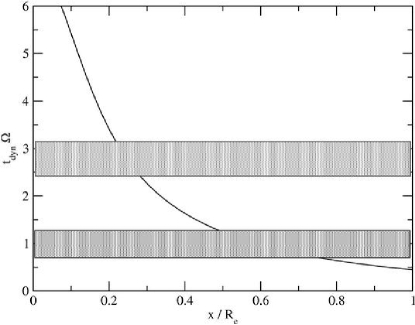
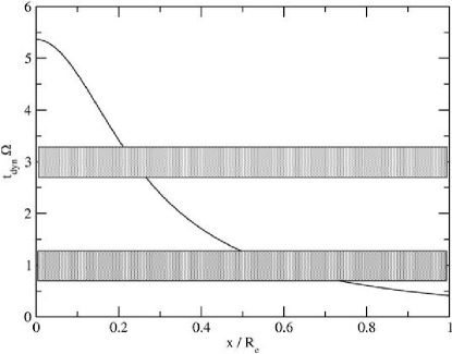
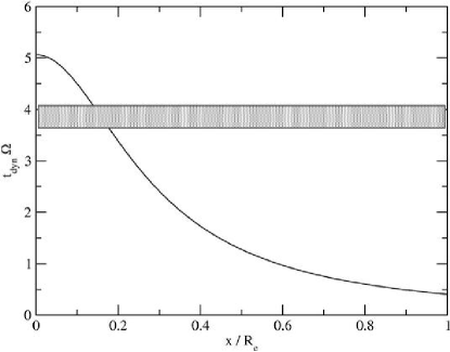
Figure 34: Angular velocity of the polytropes A0.3R0.15 (top), A0.3R0.30 (middle) and A0.3R0.40 (bottom) over the $x$ axis (black line), and approximate location of the pattern speed of the $m=1$ mode (upper rectangle) and the $m=2$ mode (lower rectangle), cf. also Fig. 15.

Fig. 34 shows the location of the unstable modes in the corotation band, for three different models on the sequence $\Gamma=4/3$, $\rho_{c}=10^{-7}$, and $A=0.3$. All modes are in corotation, but there is evidence that, for decreasing $T/|W|$, the corotation point moves towards the axis of rotation. This gives support to the arguments presented in Watts et al. (2005), where the existence of low-$T/|W|$ and spiral-arm instabilities in differentially rotating polytropes are connected to corotation. Limitations of resources did not permit us to investigate the boundary of the corotation region, where growth times of many $t_{dyn}$ are expected. However, with the results of Sections V.4 and V.8, a purely Newtonian investigation could be sufficient to reproduce the linear regime of the instability.

V.7 Evolution of a model with a slow growth of the $m=1$ instability

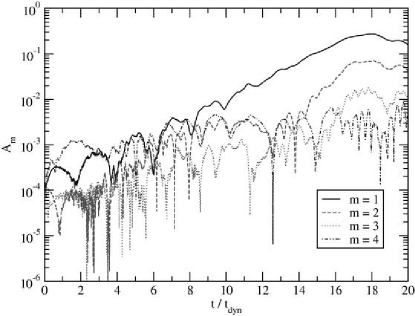
Figure 35: Long-term evolution of the mode amplitudes for the model A0.2R0.45, which is unstable to an $m=1$ perturbation. The mode, however, grows rather slowly over a time of $20\,t_{dyn}$.

As already discussed, the nature of the class “(I)” models in Fig. 25 could not be investigated in detail due to the high computational cost when evolving general relativistic, three-dimensional models. However, to illustrate the behaviour in one specific case, a long-term simulation of the model A0.2R0.45 has been performed (Fig. 35). A slowly growing $m=1$ instability is apparent in the evolution, which saturates at high amplitudes only after $20\,t_{dyn}$. While the $m=1$ mode is clearly dominant, the $m=2$ might be unstable as well. A detailed investigation of these sequences should be attempted in the limit of vanishing compactness, with a Newtonian model and preferably, with a cylindrical grid (see also the discussion in Section VI).

V.8 Evolution of a sequence of models with different compactness starting from the boundary between the regions “I” and “(I)”

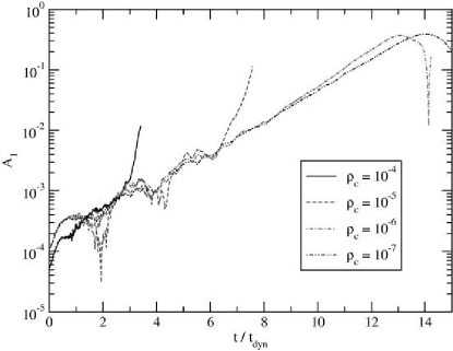
Figure 36: Amplitude of the $m=1$ mode for different models from a sequence with constant $T/|W|$ limiting in the model A0.2R0.40, which has $\rho_{c}=10^{-7}$. Cf. also Table 6.

In Section V.4, we have already studied the influence of the compactness on the development of the instability in the reference polytrope. According to the results of Section V.5, the reference model is located inside region “II” of the parameter space plane for $\rho_{c}=3.38\cdot 10^{-6}$. Thus, it is instructive to investigate the effect of compactness on a model’s evolution which is located close to the boundary between regions “I” and “(I)” in Fig. 25 (although this boundary is not sharply defined). A selected model, A0.2R0.40, has been extended to the L sequence of constant $\Gamma$, $A$, and $T/|W|$ (cf. Table 6). The influence of compactness on the $m=1$ mode is illustrated in Fig. 36: The most compact models L1 and L2 show a growth of the non-axisymmetric mode already early on, but collapse due to an axisymmetric instability (both models have $J/M^{2}<1$). The growth rate of the non-axisymmetric instability is not very sensitive to the compactness, which confirms our findings for models of the C sequence. One might therefore be reasonably optimistic that the non-axisymmetric stability properties of quasi-toroidal $N=3$ polytropes are well-represented by Fig. 25, even for a different choice of central rest-mass density. The axisymmetric stability, and the question whether the collapse of the fragment will be halted or not, is sensitive to $\rho_{c}$.

VI Discussion

In this paper we have presented an extension of our earlier work on the fragmentation of general relativistic quasi-toroidal polytropes and the production of black holes in this scenario Zink et al. (2006a). The central focus was to gain an understanding of how various parameters determining the structure of the equilibrium polytrope affect the development of the instability observed in Zink et al. (2006a), and the nature of its remnant. In addition, we have investigated the location of the unstable modes in the corotation band of the differentially rotating models.

All investigations have been performed using three-dimensional numerical simulations in general relativity, and assuming the stars to be self-gravitating perfect fluids with an adiabatic coefficient equal to the polytropic constant $\Gamma$. The equations of general relativistic hydrodynamics have been evolved using high-resolution shock-capturing methods, and the NOK-BSSN formalism has been used for the metric evolution. All grids use fixed mesh refinement, and impose an equatorial plane symmetry. The development of unstable modes has been followed by the use of a discrete Fourier transform of the rest-mass density computed at certain coordinate radii in the equatorial plane, with a preference on the radius of initial highest density.

The central results are represented in Fig. 25, 26, and 34. For a plane of constant rest-mass density $\rho_{c}=10^{-7}$ and $\Gamma=4/3$, we have determined the region where quasi-toroidal models become dynamically unstable to non-axisymmetric fragmentation. From the structure of the space of initial models presented in Fig. 4, it appears that there is a rough relation between $T/|W|$ and the highest order of unstable modes, at least as long as the degree of differential rotation is not too high. Since the numerical method is not well-suited to follow the development of instabilities with growth times much longer than a dynamical timescale, we could not determine the fate of models from class “(I)” with certainty. However, we have shown in one specific case that the model is actually unstable. In the same manner, a model from class “I” could be subject to a slowly growing mode with $m>1$; however, in this case the $m=1$ mode would clearly be dominant.

From the investigation of a sequence emanating from the model used in the publication Zink et al. (2006a), we have found that the central rest-mass density $\rho_{c}$, which controls the compactness of the polytrope, does not affect the almost exponential development of the non-axisymmetric instability significantly. This is related to the fact that $T/|W|$ is insensitive to $\rho_{c}$. However, $\rho_{c}$ determines the nature of the final remnant: While the model in Zink et al. (2006a) forms a black hole, two models having one fourth and one eighth as much compactness show a re-expansion of the fragment after maximal contraction.

The regions of models in the plane $\rho_{c}=10^{-7}$ and $\Gamma=4/3$ where such a re-expansion was observed is indicated in Fig. 26 by a “B.” If one assumes that the models not exhibiting this behaviour, marked with “C” in Fig. 26, are forming black holes in the same manner as shown in Zink et al. (2006a), then we can draw the following tentative picture of black hole formation by fragmentation of single stars.

The nature of the final system, either an almost unperturbed axisymmetric star, a single central black hole, single or multiple non-central black holes with a disk, or one or several expanding remnants without trapped surfaces, depends on the symmetry properties of the perturbation, and the location of the equilibrium star with respect to three types of surfaces in the space of parameters:

1. Surfaces indicating the onset of the instability of a mode of a certain order $m$. These surfaces might be close to isosurfaces of $T/|W|$ as indicated in Fig. 25, but the resource requirements of performing three-dimensional general relativistic simulations limit our ability to identify slowly growing modes. However, if only modes growing on a dynamical timescale are considered, then $T/|W|$ might yield a reasonable indicator of the location of the limit surfaces. The compactness of the initial model seems to have no significant effect on the location of these surfaces, at least for $\Gamma=4/3$.

2. Surfaces indicating the onset of an axisymmetric instability. In our samples, all models with $J/M^{2}<1$ were unstable to quickly growing axisymmetric modes, and hence will likely evolve to central black holes. The surface $J/M^{2}=1$ can therefore be used as an approximate separator between axisymmetric collapse and stability (cf. Sekiguchi and Shibata (2004) for a more detailed discussion of this point).

3. Surfaces separating prompt black-hole formation from re-expansion. In Fig. 26, an approximate determination of such a surface has been attempted. In a first approach, and assuming that results for the stability of slowly and uniformly rotating relativistic polytropes Durney and Roxburgh (1967); Chandrasekhar and Lebovitz (1968); Hartle et al. (1972) can be applied to the fragments, we expect a fragment with a higher compactness and lower rotation rate to be destabilized, and, given that the geometric development of the fragmentation process is similar for different choices of compactness of the equilibrium polytrope, that there is a close connection to isosurfaces of $R_{e}/M$ and $J/M^{2}$. However, when comparing the structure of $R_{e}/M$ and $J/M^{2}$ (cf. Fig. 4) and 26, the situation appears more complicated, and deserves further attention.

With respect to the question of whether multiple black holes may form or not, two comments are in order: First, in the unstable systems of class “II” and “III,” all growth times of modes with different $m$ are of comparable magnitude, i.e. the nature of the actual time development in a specific star will depend on the nature of the perturbation, as already mentioned. On a sequence of increasing $T/|W|$, we have found the $m=1$ perturbation to be dominant before higher order modes become unstable, which suggest the (off-center) formation of a single black hole with a massive accretion disk. However, as discussed in the main text, this conclusion applies to instabilities with growth times in the order of a dynamical timescale. More specifically, our simulations do not exclude, on a sequence of increasing $T/|W|$, a slowly growing higher order instability to be effective before the $m=1$ mode is dynamically unstable. Second, when two fragments are forming and collapsing, in all cases considered here a runaway instability develops and leads to a central collapse (Fig. 8). In this case, the gravitational wave signal is expected to resemble the ring-down phase of a highly deformed black hole. For the $m=1$ collapse, we have published an approximate prediction for a partial waveform in Zink et al. (2006a), which suggests an amplitude and frequency well inside the LISA sensitivity if the source is a collapsing supermassive star.

Concerning the nature of the non-axisymmetric mode, we have collected evidence that, along a sequence with decreasing $T/|W|$, the corotation point moves towards the axis of rotation of the polytrope. This gives support to the arguments by Watts et al. Watts et al. (2005). To also investigate the cases with large growth times, however, a Newtonian model, preferably on a cylindrical grid, would be of advantage to obtain more detailed results Saijo and Yoshida (2006).

A final comment is in order concerning the black hole remnant. Since the normalized angular momentum $J/M^{2}$ of the initial model is greater than unity, the resulting black hole, unless it is ejected from its shell, may very well be rapidly rotating, spun up by accretion of the material remaining outside the initial location of the trapped surface.

Possible future work on this problem can be roughly divided into four approaches. First, the nature of the low-$T/|W|$ and $m=1$ instabilities in quasi-toroidal polytropes could be investigated in Newtonian gravity, or perhaps using some perturbative approximation of general relativity, to determine the location of the corresponding surfaces in parameter space, and to suggest regions where the quantity $T/|W|$ is still a good indicator for the degree of instability. Since the Newtonian polytropes can be considered to be limit points of relativistic sequences with vanishing compactness, the systematic effects of general relativity on their stability properties can be determined separately.

Second, the location of the surfaces separating black hole formation from “bounce” behaviour, and its relation to the initial compactness $R_{e}/M$ and the normalized angular momentum $J/M^{2}$, needs to be determined with more detail, specifically also for different equations of state and rotation laws. Could a newly formed, rapidly and differentially rotating neutron star fragment in this way? We have found no example of this kind here, but such a question deserves further attention. A more detailed investigation of the “bouncing” models might also be interesting, since they could have a rich phenomenology, including a possible delayed collapse to black holes and complex gravitational wave signatures.

Third, a study of the evolution of the black hole and its shell would shed light on a number of interesting aspects: (i) The angular momentum of the remnant black hole, which is related to the structure of the accretion disk and its ability to power jets, (ii) the kick velocity of the black hole, and the question whether it may be ejected from its host galaxy in some cases, and (iii) the gravitational wave signal from the formation process at $\mathscr{J}^{+}$. While we were not able to evolve the black hole for an extended time after its formation, recent advances in discrete techniques may be able to solve this problem, either by adding a sufficient amount of artificial dissipation Baiotti and Rezzolla (2006) or by employing multi-block grids with summation-by-parts operators Lehner et al. (2005); Zink et al. (2006b).

Fourth, to connect more closely to certain astrophysical systems, a detailed model of the micro-physical processes, particle transport, and magnetic fields is necessary in many cases to obtain specific answers. The most important bulk property appears to be a change in $\Gamma$ with density, since this would modify the non-linear evolution of the fragmentation significantly. In the specific case of core collapse, results in this context have been obtained already Shibata and Sekiguchi (2005); Ott et al. (2005).