Anthropic predictions for vacuum energy and neutrino masses in the light of WMAP-3

Abstract

Anthropic probability distributions for the cosmological constant $\Lambda$ and for the sum of neutrino masses $m_{\nu}$ are updated using the WMAP-3 data release. The new distribution for $\Lambda$ is in a better agreement with observation than the earlier one. The typicality of the observed value, defined as the combined probability of all values less likely than the observed, is no less than 22%. We discuss the dependence of our results on the simplifying assumptions used in deriving the distribution for $\Lambda$ and show that the agreement of the anthropic prediction with the data is rather robust. The distribution for $m_{\nu}$ is peaked at $m_{\nu}\sim 1$ eV, suggesting degenerate neutrino masses, but a hierarchical mass pattern is still marginally allowed at a $2\sigma$ level.

I Introduction

The parameters we call constants of Nature may in fact be stochastic variables taking different values in different parts of the universe. The observed values are then determined by chance and by anthropic selection. Recent developments in string theory Bousso ; Susskind03 , combined with the ideas of eternal inflation AV83 ; Linde86 , have led to the ”landscape” paradigm, which provides a theoretical basis for this picture. And the successful prediction of a nonzero cosmological constant $\Lambda$ Weinberg87 ; Linde87 ; AV95 ; Efstathiou95 ; Weinberg97 ; MSW may be our first evidence for the existence of a huge multiverse beyond our horizon. (For an up to date discussion of these ideas, see Carr .)

Anthropic predictions are necessarily statistical in nature. Even though the observed value of $\Lambda$ is within the expected range, there is a lingering doubt that this may be no more than a lucky guess. To further test the theory, we should try to extract predictions for variables other than $\Lambda$. Some attempts in this direction have already been made. Predictions for the neutrino masses $m_{\nu}$ have been discussed in TVP03 ; PVT04 , and a postdiction for the (axionic) dark matter mass per baryon, $\xi$, has been given in Wilczek .

A reliable calculation of anthropic probability distributions is a very challenging task. All calculations performed so far have relied on a number of simplifying assumptions. Moreover, the form of the distributions for $\Lambda$ and $m_{\nu}$ depends on the values of the cosmological parameters: the Hubble parameter $h$, the tilt of the perturbation spectrum $n_{s}$, and particularly on $\sigma_{8}$ – the amplitude of linear density perturbations on the scale of $8h^{-1}$ Mpc. Hence, the agreement (or disagreement) of the predictions with the data should be regarded as tentative. With improved understanding or improved measurements, it may either get better or worse.

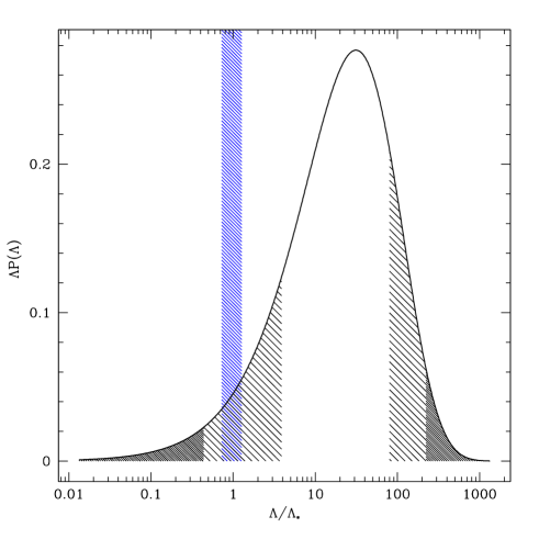
Figure 1: The probability distribution for $\Lambda$ based on the flat $\Lambda$CDM best fit parameters from WMAP-1. $\Lambda_{*}$ is the observed value whose $1\sigma$ uncertainty is represented by the blue shaded vertical stripe.

In Fig. 1 we show the distribution $P(\Lambda)$ circa 2005. Its calculation has been discussed in AV95 ; Efstathiou95 ; AV96 ; Weinberg97 ; MSW ; GV03 ; GLV03 . The parameter values used in the figure were based primarily on the first year of WMAP data. The agreement between the theory and observation can be characterized by the “typicality” of the observed value $\Lambda_{*}$, ${\cal T}(\Lambda_{*})$ Page . (The definition of typicality will be discussed in Section II.) For the distribution in Fig.1, ${\cal T}(\Lambda_{*})\approx 10$%. For a statistical model of this sort, this can be regarded a good agreement.

With the release of the 3-year WMAP data, some of the parameters (such as $n_{s}$ and $h$) are now known with a better accuracy. Among implications was a decrease in the value of $\sigma_{8}$ by more than 10%, from $0.9\pm 0.1$wmap1 to $0.76\pm 0.05$wmap3 . Combining other datasets with the WMAP data can change the preferred values of the parameters. For example, adding all available information, including the SDSS Lyman-$\alpha$ forest data mcdonald05 , was reported to increase the value of $\sigma_{8}$ to $0.85\pm 0.02$ seljak06 . On the other hand, combining the WMAP data with the distribution of SDSS luminous red galaxies yields $\sigma_{8}=0.76\pm 0.03$ tegmark_lrg in good agreement with results of the WMAP team. Here, as in our original analysis, we will make use of the WMAP data alone, which is most likely to be free of systematics and, for the flat power law $\Lambda$CDM model, provides sufficiently accurate measurements of the spectral index and other cosmological parameters that determine $\sigma_{8}$.

The main goal of the present paper is to update the distributions for $\Lambda$ and $m_{\nu}$ using the WMAP-3 data. We shall see that both distributions are shifted toward smaller values of $\Lambda$ and $m_{\nu}$, respectively. The agreement between theory and observations is improved as a result. We shall also discuss the dependence of the results on the simplifying assumptions made in the calculation of probabilities.

In the next section, we discuss the concept of typicality which will be used as a quantitative measure of the agreement of theoretical distributions with the data. The case where $\Lambda$ is the only variable is considered in Section III. The effects of other variable parameters, such as the amplitude of the primordial density perturbations $Q$ and the dark matter mass per photon $\xi$, and the dependence on the assumed value of the galactic mass $M_{G}$, are discussed in IV. Variable $m_{\nu}$ and joint variation of $m_{\nu}$ and $\Lambda$ is analyzed in Section V. We finish with some concluding remarks in Section VI.

II Typicality

Figure 2: Values “less probable” than $X_{*}$ are located in the two shaded regions, which have equal measure in the distribution $P(X)$.

Consider a variable $X$ defined in the interval $a<X<b$ and characterized by a probability distribution $P(X)$. The value $X=X_{*}$ has typicality ${\cal T}$ if ${\cal T}$% of the distribution are “less probable” than $X_{*}$. Page Page assumes that the least probable values are at the tails of the distribution (see Fig. 2). The motivation is that such values are fine-tuned to be near the special points $a$ and $b$, which are the endpoints of the interval.

Suppose for definiteness that $X_{*}$ is closer to $a$ than to $b$ in terms of the measure $P(X)$, so that

$$P_{*}\equiv\int_{a}^{X_{*}}P(X)dX<{1\over{2}}.$$ (1)

Let us also define ${X_{*}}^{\prime}$, which is equally close to $b$,

$$\int_{{X_{*}}^{\prime}}^{b}P(X)dX=P_{*}.$$ (2)

The values in the intervals $a<X<X_{*}$ and ${X_{*}}^{\prime}<X<b$ are regarded as less likely than $X_{*}$. The typicality is then given by

$${\cal T}(X_{*})=2P_{*}.$$ (3)

In the case of the cosmological constant, apart from the vicinity of the endpoints at $\Lambda=\pm\infty$, there is an additional range of unlikely values near zero. $\Lambda=0$ is a special value, which defines the boundary between eternal expansion and recollapse. Having $\Lambda$ accidentally fine-tuned very close to this point is unlikely, and we want this reflected in the typicality. We shall define $P_{*}$ as the “distance”, in terms of the measure $P(\Lambda)$, from the observed value $\Lambda_{*}$ to the nearest special point $(\Lambda=0,\pm\infty)$. It will also be convenient to define the probabilities $P_{\pm}$ for positive and negative $\Lambda$,

$$P_{+}=\int_{0}^{\infty}P(\Lambda)d\Lambda,$$ (4)

$$P_{-}=\int_{-\infty}^{0}P(\Lambda)d\Lambda,$$ (5)

$P_{+}+P_{-}=1$. A straightforward generalization of Page’s definition is to define typicality as the measure of all points whose distance to the nearest special point is less than $P_{*}$.

It is clear from Fig. 1 that the special point closest to the observed value $\Lambda_{*}$ is $\Lambda=0$. Hence,

$$P_{*}=\int_{0}^{\Lambda_{*}}P(\Lambda)d\Lambda<P_{+}/2.$$ (6)

If in addition $P_{*}<P_{-}/2$, then there are four intervals of $\Lambda$ less likely than $\Lambda_{*}$, each having measure $P_{*}$, and thus

$${\cal T}(\Lambda_{*})=4P_{*}.$$ (7)

Alternatively, if $P_{*}>P_{-}/2$, we have

$${\cal T}(\Lambda_{*})=P_{-}+2P_{*}.$$ (8)

Most of the calculations of the distribution $P(\Lambda)$ have been performed for $\Lambda>0$. For negative $\Lambda$, the universe recollapses at $t_{\Lambda}=(6\pi G|\Lambda|)^{-1/2}$. To find the distribution in this case, we need to know the probability for a civilization to evolve during this time interval, which is of course very uncertain. It is very likely, however, that positive $\Lambda$ are more probable than negative $\Lambda$ Weinberg05 ,

$$P_{+}>P_{-}.$$ (9)

Note, for example, that for $\Lambda=-20\Lambda_{*}$ the universe would recollapse in 3 billion years. Star formation in such a universe will not begin before the onset of the recollapse, and the remaining 1.5 billion years are hardly sufficient to disperse heavy elements in supernova explosions, form planetary systems and evolve intelligent life. On the other hand, the 2$\sigma$ range for positive $\Lambda$ extends to $80\Lambda_{*}$. The inequality (9) can be used to derive a lower bound on ${\cal T}(\Lambda_{*})$.

Let ${\cal T}_{+}(\Lambda_{*})$ be the typicality calculated in the interval $0<\Lambda<\infty$ with $P(\Lambda)$ normalized in that interval,

$${\cal T}_{+}(\Lambda_{*})=2P_{*}/P_{+}.$$ (10)

Now, using Eq. (9) it is easily verified that

$${\cal T}(\Lambda_{*})>{\cal T}_{+}(\Lambda_{*}).$$ (11)

In the rest of the paper we shall consider only positive $\Lambda$ and the corresponding typicality ${\cal T}_{+}$. According to (11), it can be regarded as a lower bound for the full typicality ${\cal T}$.

III The probability distribution for $\Lambda$

The method used in this paper follows closely that in MSW ; GV03 ; TVP03 ; PVT04 . Here we only reproduce the essential details and refer the reader to PVT04 for a comprehensive description. Consider a model in which $\Lambda$ is allowed to vary from one part of the Universe to another. We define the distribution ${\cal P}(\Lambda)d\Lambda$ as the probability for a randomly picked observer to measure $\Lambda$ in the interval $d\Lambda$. This distribution can be represented as

$$P(\Lambda)=P_{prior}(\Lambda)f_{selec}(\Lambda),$$ (12)

where the prior probability $P_{prior}(\Lambda)$ is determined by the geography of the landscape and by the dynamics of eternal inflation, and $f_{selec}(\Lambda)$ accounts for anthropic selection effects.

The standard argument AV96 ; Weinberg97 suggests that the prior probability is well approximated by

$$P_{prior}\approx{\rm const},$$ (13)

because the anthropic range where $f_{selec}(\Lambda)$ is appreciably different from zero is much narrower than the full range of $\Lambda$. We emphasize that this is just a heuristic argument. The conditions for its validity have been discussed both in scalar field models, where $\Lambda$ is a continuous parameter GV00 ; Weinberg00 ; GV01 ; GV03 , and in “discretuum” models with a large set of metastable vacua Delia1 ; Delia2 . Future work will show whether or not these conditions are satisfied in the string theory landscape. Here we shall assume that Eq.(13) is valid.

It has been the standard practice to identify the selection factor in (12) with the asymptotic fraction of baryonic matter, $F(M>M_{G},\Lambda)$, which clusters into objects of mass greater than the characteristic galactic mass $M_{G}\sim 10^{12}M_{\odot}$:

$$f_{selec}(\Lambda)\propto F(M>M_{G},\Lambda).$$ (14)

The idea here is that there is a certain average number of stars per unit baryonic mass and a certain number of observers per star, and that these numbers are not strongly affected by the value of $\Lambda$. In the present Section we shall adopt this standard approach; its validity will be analyzed in Section III.

The fraction of collapsed matter $F(M>M_{G},\Lambda)$ can be approximated using the Press-Schechter (PS) formalism PressSchechter . This leads to

$$F(M>M_{G},\Lambda) \propto {\rm erfc}\,\left[{X\over\sqrt{2}}\right],$$ (15)

where

$$X=\delta_{c}/{\sigma_{\infty}(\Lambda)}\ ,$$ (16)

$\delta_{c}\approx 1.63$ and $\sigma_{\infty}$ is the variance of the Gaussian density fluctuation field in the asymptotic future on the galactic scale $M_{G}$. The latter quantity can be written as PVT04

$$\sigma_{\infty}(\Lambda)={\sigma_{G}^{*}}{D^{\infty}(\Lambda)\over{D}(\Lambda_{*},x_{*})}\ .$$ (17)

Here, ${\sigma}_{G}^{*}$ is the current density contrast on the galactic scale $M_{G}$ inferred from the large-scale CMB data, $x_{*}$ is our local value of $\Omega_{\Lambda}/\Omega_{M}$, $\Lambda_{*}$ is the local value of vacuum energy density, $D(\Lambda_{*},x_{*})$ is the local linear growth factor and $D^{\infty}(\Lambda)\equiv D(\Lambda,x=\infty)$.

N-body simulations indicate that the PS model overestimates the abandance of “typical” halos, while underestimating that of more massive structures jenkins01 . The Sheth-Tormen model ST99 was shown to fit the simulations better. We have checked that replacing the PS formula with that of ST99 does not significantly affect our results and use the PS model through out this work.

To evaluate ${\sigma}_{G}^{*}$ we first find the length scale $R(M_{G})$ corresponding to the mass scale $M_{G}$ using

$$R(M_{G}) = \left({3M_{G}\over 4\pi\rho_{0}}\right)^{1/3}$$ (18)

$$\approx 0.951\ \left({h\over\Omega_{M}}\right)^{1/3}\left({M_{G}\over 10^{12}M_{\odot}}\right)^{1/3}{\rm h^{-1}Mpc}\ ,$$

where $\rho_{0}\approx 1.88\cdot 10^{-26}\ {\Omega_{M}h^{2}}\ {\rm kg/m}^{3}$ is the mean cosmic density of nonrelativistic matter. For $h=0.73$ and $\Omega_{M}=0.234$ this gives

$$R(M_{G})\approx 1.4\ {\rm h^{-1}Mpc}\left({M_{G}\over 10^{12}M_{\odot}}\right)^{1/3}\ .$$ (19)

The corresponding linearized density contrast ${\sigma}_{G}^{*}$ found using WMAP-3’s best fit power law model wmap3 for $M=10^{12}M_{\odot}$ is

$${\sigma}_{G}^{*}\equiv\sigma[R(M_{G})]=\left[{1\over 2\pi^{2}}\int_{0}^{\infty}P(k)W^{2}(kR)k^{2}dk\right]^{1/2}\approx 1.87\pm 0.13\ .$$ (20)

In the above, $P(k)$ is today’s linear matter power spectrum and $W(kR)$ is the window function. We work with the “top-hat” form for $W(kR)$, also used by the WMAP team. This value is smaller than ${\sigma}_{G}^{*}\approx 2.41\pm 0.26$ inferred from the WMAP-1 data and used in TVP03 ; PVT04 .

The growth factor $D(\Lambda,x)$ in a universe containing only $\Lambda$ and pressureless matter can be written as heath77 ; MSW

$$D(\Lambda,x)=1+{3\over 2}{x_{eq}}^{-1/3}G(x)\ ,$$ (21)

where

$$G(x)={5\over 6}\left[1+x\over x\right]^{1/2}\int_{0}^{x}{dw\over w^{1/6}\ (1+w)^{3/2}}\ .$$ (22)

Using ${3\over 2}{x_{eq}}^{-1/3}G(x)\gg 1$, the variable $X$ defined in Eq. (16) can be written as

$$X={\delta_{c}\over\sigma_{G}^{*}}\left(\Lambda\over\Lambda_{*}\right)^{1/3}{G(x_{*})\over G(\infty)}\ .$$ (23)

The variance $\sigma_{G}^{*}$ is proportional to the amplitude of primordial fluctuations $Q$. The dependence on Q can be explicitly introduced by writing

$$\sigma_{G}=\sigma_{G}^{*}{Q\over Q_{*}}\ ,$$ (24)

where $Q_{*}$ is the observed value of $Q$. We follow the WMAP-3 team’s conventions wmap3 and define $Q\equiv\Delta_{k}(k=0.002{\rm h/Mpc})$ with the best fit value of $Q_{*}=4.9\times 10^{-5}$. Then $X$ can be written as

$$X=A\left(\Lambda\over\Lambda_{*}\right)^{1/3}{1\over Q}\ ,$$ (25)

with

$$A\approx 3.2\times 10^{-5}\left(M_{G}\over 10^{12}M_{\odot}\right)^{0.1}\ ,$$ (26)

where the mass dependence of $A$ comes from that of $\sigma_{G}^{*}$ in (20) and the approximation is valid for values of $M_{G}$ within a few orders of magnitude of $10^{12}M_{\odot}$.

In summary, the distribution for $\Lambda$ is

$$P(\Lambda)d\Lambda\propto{\rm erfc}\,\left[{X\over{\sqrt{2}}}\right]d\Lambda,$$ (27)

where $X$ is given by Eq. (25) with $A$ from Eq. (26).

The degree of clustering that we observe today is often parameterized by the variance of the linear density contrast field on the $8h^{-1}$Mpc scale, $\sigma_{8}$. The latest observations, as mentioned in the introduction, indicate a lower value of $\sigma_{8}$, and correspondingly a lower value of $\sigma_{G}$. A decrease in $\sigma_{G}$ at a fixed $\Lambda$ leads to a suppression of galaxy formation, except for very small values of $\Lambda$, such that $\Lambda$-domination occurs when clustering on the galactic scale is essentially complete. As a result the peak of the probability distribution is shifted towards lower values, leading to a better agreement with the observed $\Lambda$.

The updated distribution is shown in Figure 3 and corresponds to a typicality of ${\cal T}_{+}=22$% for our local value of $\Lambda$.

In Weinberg05 Weinberg reports a probability of $15.6$% for the observed value of $\Lambda$, implying a typicality ${\cal T}_{+}=31$%. (His probability includes only values between $0$ and $\Lambda_{*}$; it is half of what we call ${\cal T}_{+}$.) This result is based on the WMAP-1 data and is higher because of the use of the Gaussian window function with $R_{G}=2$ Mpc. This corresponds (for the same mass) to an effective ”top-hat” radius of $R(M_{G})\approx 2.3$ Mpc/h (as opposed to 1.4 Mpc/h used in this paper). For the WMAP-3 parameters Weinberg’s calculation would yeild a typicality around $50$%.

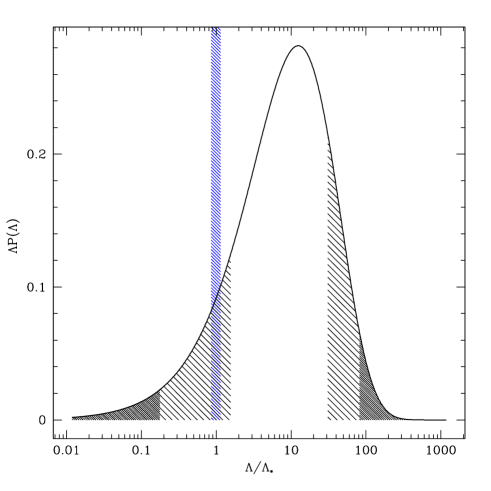
Figure 3: The probability distribution for $\Lambda$ obtained as in Fig. 1 but using parameters derived from the WMAP-3 data. The observed value, $\Lambda_{*}$, has a typicality of $22$%.

IV Dependence on simplifying assumptions

The calculation of $P(\Lambda)$ that led to the distribution in Fig. 3 relied on a number of simplifying assumptions. In particular, we assumed (i) that $\Lambda$ is the only variable parameter and (ii) that the number of observers is proportional to the mass fraction in giant galaxies of mass greater than $M_{G}=10^{12}M_{\odot}$. We shall now discuss how sensitive our conclusions are to these assumptions and what modifications we can expect in more realistic models.

IV.1 Other variable parameters

A criticism that has often been raised against the anthropic prediction of $\Lambda$ is that the agreement of the prediction with the data is destroyed if one allows parameters other than $\Lambda$ to vary. For example, if the amplitude of the primordial density perturbations $Q$ is also variable, then galaxies will form earlier in regions with larger $Q$, and $\Lambda$ can take larger values without interfering with galaxy formation Banks . However, it has been shown in Livio that the probability distribution in this case factorizes as

$$P(Q,\Lambda)dQd\Lambda=P_{prior}(Q)~{}{\rm erfc}\,\left[{X\over{\sqrt{2}}}\right]dQd\Lambda\propto Q^{3}P_{prior}(Q)dQ~{}{\rm erfc}\,\left[{X\over{\sqrt{2}}}\right]X^{2}dX.$$ (28)

Here the factors $Q^{3}$ and $X^{2}$ come from the transformation Jacobian and we have used the expression for $X$ in Eq. (25).

The value of $Q$ is determined by the shape of the inflaton potential, and the prior distribution for $Q$ is highly model-dependent Hall1 ; catastrophe ; Hall2 . So it is very fortunate that the $Q$-dependent part of the distribution has completely factored out, and we are left with the distribution for $X$,

$$P(X)dX\propto{\rm erfc}\,\left[{X\over{\sqrt{2}}}\right]d(X^{3}).$$ (29)

For a fixed $Q$, $X^{3}\propto\Lambda$ with a constant coefficient, and we recover Eq. (27). For a variable $Q$, Eq. (29) shows that the distribution has exactly the same form, except now it should be regarded as a distribution for the variable $X^{3}\propto\Lambda/Q^{3}$. The typicality of the observed value of $X$ is therefore the same as what we found for $\Lambda_{*}$ in the preceding section, ${\cal T}(X_{*})=22\%$.

This conclusion can be extended to include a variable dark matter mass per photon, $\xi$. Using the analysis in Wilczek , it can be shown that, to a good approximation, the distribution in this case can still be factorized into a part depending on $Q$ and $\xi$ and a part depending on $X^{3}\propto\Lambda/Q^{3}\xi^{4}$. The predicted range of $X$ is unaffected by variation of $Q$ and $\xi$ and is independent of their prior distributions.

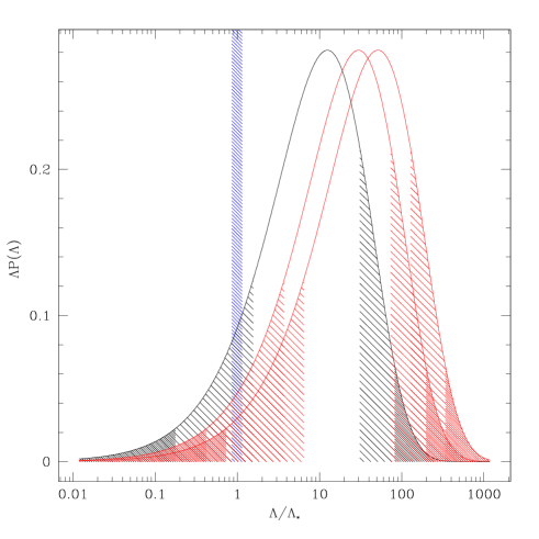
Figure 4: The probability distribution for $\Lambda$ assuming three different mass thresholds for halos that can become habitable galaxies. From left to right, the curves correspond to thresholds of $10^{12}M_{\odot}$, $10^{11}M_{\odot}$ and $10^{10}M_{\odot}$ . The typicalities of the observed value, $\Lambda_{*}$, are $22$%, $11$% and $7$%, respectively.

IV.2 Dependence on the characteristic mass scale $M_{G}$

Next we investigate the dependence of $P(\Lambda)$ on the galaxy mass cutoff $M_{G}$. It has been argued by Loeb Loeb06 that the anthropic explanation of $\Lambda$ would be significantly weakened if a large number of habitable planets were found to exist in smaller galaxies, such as the dwarf descendants of galaxies formed at $z\sim 10$. It would mean that planet-based observers could be abundant in our Universe even if the cosmological constant was some orders of magnitude larger than observed.

One motivation for introducing the cutoff mass $M_{G}$ is that, in the hierarchical structure formation scenario, smaller galaxies typically form at earlier times and have a higher density of matter. This may increase the danger of nearby supernova explosions and the rate of near encounters with stars, large molecular clouds, or clumps of dark mater TR98 ; GV03 ; Wilczek . Gravitational perturbations of planetary systems in such encounters could send a rain of comets from the Oort-type clouds toward the inner planets, causing mass extinctions. (Encounters close enough to disrupt planetary orbits are much less likely.) With the present rate of mass extinctions (about once in $10^{8}$ yrs), the intervals between these events are already comparable to the time it took humans to evolve. Hence, a substantial increase of the rate may result in a suppression of the number of observers.

Another consideration is that the properties of galaxies, as a function of their mass, are observed to undergo a sharp transition at the halo mass of about $M_{h}\sim 2\times 10^{11}M_{\odot}$ (stellar mass $\sim 3\times 10^{10}M_{\odot}$) Kauffmann . For larger masses, baryons are efficiently converted into stars, while for smaller masses the efficiency is lower and decreases as $M$ gets smaller. The metallicity is also observed to drop with mass Tremonti03 : dwarf galaxies appear to be deficient in heavy elements, which are necessary for the formation of planets. These traits are attributed to supernova feedback: supernova explosions either expel a fair fraction of gas from low-mass galaxies or inhibit star formation. (For a discussion and references, see Deckel ). Low mass fraction in stars and low metallicity indicate that dwarf galaxies are less likely to harbor observers.

The effective cutoff mass $M_{G}$ cannot be determined without a quantitative study of these effects. We shall not attempt this here. In order to quantify the dependence of our predictions on the value of $M_{G}$, we repeated the analysis in Section III using two lower values, namely, $10^{11}M_{\odot}$ and $10^{10}M_{\odot}$. The resulting distributions are shown in Fig. 4.

As expected, a decrease of $M_{G}$ shifts the distribution towards larger values of $\Lambda$. However, the effect is not dramatic. The observed value remains in the 95% range of the distribution. Its typicality ${\cal T}_{+}$ is reduced from 22% for $M_{G}=10^{12}M_{\odot}$ to $11$% and $7$% (for $M_{G}=10^{11}M_{\odot}$ and $M_{G}=10^{10}M_{\odot}$, respectively).

V Variable $m_{\nu}$ and joint variation of $m_{\nu}$ and $\Lambda$

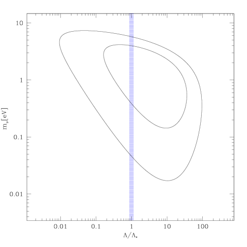
Figure 5: The $68$ and $95$% joint probability contours for $\Lambda$ and $m_{\nu}$ obtained using the WMAP-3 parameters.

Figure 6: The probability distribution for the sum of the neutrino masses, $m_{\nu}$, obtained using the WMAP-3 parameters.

We now consider the case when both the sum of the neutrino masses, $m_{\nu}\equiv m_{1}+m_{2}+m_{3}$, and the vacuum energy density, $\Lambda$, vary from one part of the Universe to another. The possibility that the smallness of the neutrino masses may be due to anthropic selection has been first suggested in TVP03 . The mass-squared differences of the three neutrino species are now known with an accuracy of about 10%,

$$\Delta m_{32}^{2}\approx 2.6\times 10^{-3}~{}eV^{2},$$ (30)

$$\Delta m_{21}^{2}\approx 8\times 10^{-5}~{}eV^{2}.$$ (31)

The absolute values of the neutrino masses are currently unknown. This makes them an ideal target for anthropic predictions.

It is usually assumed that the neutrino mass eigenvalues form a “normal” hierarchy, i.e., $m_{1}\ll m_{2}\ll m_{3}$. Then it follows from Eqs. (30),(31) that $m_{\nu}\sim 0.06~{}eV$. The opposite regime is when the three masses are degenerate, $m_{1}\approx m_{2}\approx m_{3}$. An intermediate case is that of inverted hierarchy, $m_{3}\ll m_{2}\approx m_{1}$, in which case $m_{\nu}\approx 0.11$ eV. The astrophysical upper bound from the WMAP-3 data is $m_{\nu}\lesssim 2~{}eV$. Stronger bounds have been quoted from combined astrophysical data sets, but their validity is not certain (for a recent review see Fogli06 ).

Assuming that $m_{\nu}$ and $\Lambda$ vary independently, their joint prior probability is a product of the individual priors. We have already chosen a flat prior for $\Lambda$ in Section III. The prior probability for $m_{\nu}$ was discussed in TVP03 ; PVT04 with the conclusion that ${\cal P}_{prior}(m_{\nu})={\rm const}$ is the best motivated choice. As in Section III, we approximate the anthropic selection factor as the asymptotic mass fraction in galaxies of mass $M>M_{G}$,

$$f_{selec}(m_{\nu},\Lambda)\propto F(M>M_{G},m_{\nu},\Lambda) \propto {\rm erfc}\,\left[{X\over\sqrt{2}}\right],$$ (32)

where

$$X={\delta_{c}\over\hat{\sigma}(M)}{{\hat{D}}(f_{{\nu}*},\Lambda_{*},x_{*})\over D^{\infty}(f_{\nu},\Lambda)}\ .$$ (33)

The notation above is similar to that of Eq. (17) of Section III, except for the hats indicating the quantities evaluated for our local region assuming massless neutrinos. We refer the reader to PVT04 for a detailed derivation of the above expressions. The updated joint probability distribution for $\Lambda$ and $m_{\nu}$ is shown in Figure 5.

It is of interest to also evaluate the anthropic prediction for $m_{\nu}$ under the assumption of fixed $\Lambda=\Lambda_{*}$. This distribution is shown in Figure 6. The difference, compared to the results in TVP03 , is that the mean value of $m_{\nu}$ has decreased from $2.1$eV to $1.5$eV, and the lower boundary of the $2\sigma$ region from $0.07$ eV to $0.05$eV.

Both the single-variable and combined distributions are peaked at a value $m_{\nu}\sim 1$ eV, corresponding to degenerate neutrino masses. The $1\sigma$ range of the distribution, $0.3~{}eV<m_{\nu}<3~{}eV$, also predicts degeneracy. The prediction, however, is not very strong: the $2\sigma$ range is (marginally) consistent with the hierarchical mass pattern. We note that for $m_{\nu}\sim 1$ eV the observed value of $\Lambda$ is well within the $1\sigma$ range of the distribution.

VI Discussion

The observed value of the cosmological constant, $\Lambda_{*}$, is mysterious for two reasons. First, all particle physics estimates yield enormous values, many orders of magnitude greater than $\Lambda_{*}$. Second, $\Lambda_{*}$ is comparable to the average matter density at the present epoch – a coincidence calling for an explanation. Both of these facts are accounted for in the multiverse model, where $\Lambda$ is a variable changing from one place in the universe to another. Despite many attempts, there are no plausible alternative explanations. A satisfactory agreement between the observed $\Lambda_{*}$ and the anthropic prediction is therefore hard to dismiss. It may be our first evidence for the existence of the multiverse.

In this paper we have updated the anthropic probability distribution for $\Lambda$ using the WMAP-3 data release. This resulted in an improved agreement between the theory and the data. The typicality of the observed value $\Lambda_{*}$, defined as the probability of all values “less likely” than $\Lambda_{*}$, is ${\cal T}_{+}(\Lambda_{*})=22\%$. (As we explained in Sec. II, this estimate should be regarded as a lower bound, since our analysis did not include negative $\Lambda$.)

We analyzed the dependence of the successful prediction for $\Lambda$ on the simplifying assumptions used to derive the distribution $P(\Lambda)$. Our conclusion is that the prediction is rather robust. It is not drastically modified by variation of the cutoff galactic mass $M_{G}$ and remains essentially unaffected by inclusion of other anthropic variables, such as the amplitude of primordial density perturbations $Q$, or mass of dark matter per baryon $\xi$. Variation of the sum of the neutrino masses $m_{\nu}$ does have some effect on $P(\Lambda)$. As $m_{\nu}$ is increased from its lowest value, the agreement with the data improves, and for $m_{\nu}\sim 1$ eV the observed value $\Lambda_{*}$ is well within the $1\sigma$ range of the distribution.

We have also updated the anthropic prediction for $m_{\nu}$. With a flat prior, the distribution is peaked at $m_{\nu}\sim 1$ eV, suggesting degenerate neutrino masses. A hierarchical neutrino mass pattern is marginally acceptable at the $2\sigma$ level.

Unlike the case of the cosmological constant, there is a viable alternative explanation for the smallness of the neutrino masses. It is the see-saw mechanism. We note that a recent study failed to find models exhibiting this mechanism in a wide class of string theory inspired models Langacker . We note finally that a value of $m_{\nu}\sim 1$ eV is suggested by the Heidelberg-Moscow double beta decay experiment doublebeta . This claim, however, remains controversial controversial .

- (1) R. Bousso and J. Polchinski, JHEP 0006:006 (2000).
- (2) L. Susskind, hep-th/0302219 (2003).
- (3) A. Vilenkin, Phys. Rev. D27, 2848 (1983).
- (4) A. D. Linde, Phys. Lett. 175B, 395 (1986).
- (5) S. Weinberg, Phys. Rev. Lett. 59, 2607 (1987).
- (6) A.D. Linde, in 300 Years of Gravitation, ed. by S.W. Hawking and W. Israel, Cambridge University Press, Cambridge (1987).
- (7) A. Vilenkin, Phys. Rev. Lett. 74, 846 (1995).
- (8) G. Efstathiou, MNRAS 274, L73 (1995).
- (9) S. Weinberg, in “Critical Dialogues in Cosmology”, proceedings of a Conference held at Princeton, New Jersey, 24-27 June 1996, Singapore: World Scientific, edited by Neil Turok, 1997., p.195.
- (10) H. Martel, P.R. Shapiro and S. Weinberg, Ap. J. 492, 29 (1998).
- (11) Universe or Multiverse, ed. by B.J. Carr (Cambridge University Press, in press).
- (12) M. Tegmark, A. Vilenkin, and L. Pogosian, astro-ph/0304536, Phys.Rev. D71, 103523 (2005).
- (13) L. Pogosian, A. Vilenkin, and M. Tegmark, astro-ph/0404497, JCAP 0407 (2004) 005.
- (14) M. Tegmark, A. Aguirre, M.J. Rees and F. Wilczek, astro-ph/0511774.
- (15) A. Vilenkin, in Cosmological constant and the evolution of the universe, ed by K. Sato, T. Suginohara and N. Sugiyama (Universal Academy Press, Tokyo, 1996); gr-qc/9512031.
- (16) J. Garriga and A. Vilenkin, Phys. Rev. D67, 043503 (2003).
- (17) J. Garriga, A.D. Linde and A. Vilenkin, Phys. Rev. D69, 063521 (2004).
- (18) D. N. Page, in Carr , arXiv:hep-th/0610101.
- (19) D. N. Spergel et al (WMAP-1), Astrophys.J.Suppl. 148 (2003) 175.
- (20) D. N. Spergel et al (WMAP-4), astro-ph/0603449, submitted to Ap. J.
- (21) P. McDonald et al, Astrophys.J. 635 (2005) 761.
- (22) U. Seljak, A. Slosar, P. McDonald, astro-ph/0604335.
- (23) M. Tegmark et al (SDSS), astro-ph/0608632.
- (24) S. Weinberg, hep-th/0511037, to be published in “Universe or Multiverse”, ed. B. Carr (Cambridge University Press).
- (25) J. Garriga and A. Vilenkin, Phys. Rev. D61, 083502 (2000).
- (26) S. Weinberg, Phys. Rev. D61, 103505 (2000).
- (27) J. Garriga and A. Vilenkin, Phys. Rev. D64, 023517 (2001).
- (28) D. Schwartz-Perlov and A. Vilenkin, JCAP 0606, 010 (2006) [arXiv:hep-th/0601162].
- (29) K. Olum and D. Schwartz-Perlov, in preparation.
- (30) W. H. Press and P. Schechter, ApJ 187, 425 (1974).
- (31) A. Jenkins et al,MNRAS 321, 372 (2001).
- (32) R. K. Sheth and G. Tormen, MNRAS 308, 119 (1999); R. K. Sheth,H. J. Mo, and G. Tormen, astro-ph/9907024.
- (33) D. J. Heath, MNRAS 179, 351 (1977).
- (34) T. Banks, M. Dine and E. Gorbatov, JHEP 0408, 058 (2004).
- (35) J. Garriga, M. Livio and A. Vilenkin, Phys. Rev. D61, 023503 (2000).
- (36) B. Feldstein, L.J. Hall and T. Watari, Phys. Rev. D72, 123506 (2005).
- (37) J. Garriga and A. Vilenkin, Prog. Theor. Phys. Suppl. 163, 245 (2006).
- (38) L.J. Hall, T. Watari and T.T. Yanagida, Phys. Rev. D73, 103502 (2006).
- (39) A. Loeb, “An Observational Test for the Anthropic Origin of the Cosmological JCAP 0605, 009 (2006) [arXiv:astro-ph/0604242].
- (40) M. Tegmark and M. Rees, Ap. J. 499, 526 (1998).
- (41) G. Kauffmann et. al., MNRAS 341, 54 (2003).
- (42) C.A. Tremonti et. al., Ap. J. 613, 898 (2004).
- (43) A. Deckel and J. Woo, MNRAS 344, 1131 (2003).
- (44) G.L. Fogli et. al., hep-ph/0608060.
- (45) J. Giedt, G.L. Kane, P. Langacker and B.D. Nelson,, Phys. Rev. D71, 115013 (2005).
- (46) H.V. Klapdor-Kleingrothaus, I.V. Krivosheina, A. Dietz and O. Chkvorets, Phys. Lett. B586, 198 (2004).
- (47) S.R. Elliott and J. Engel, J. Phys. G 30, R183 (2004).